Overview
This edition follows the 29-page arXiv v2 dated 7 October 2026, retaining all 12 numbered figures, 16 tables, four equations and 37 references. Visible Touch renders tactile signals onto the camera images already consumed by a policy. The reported +30.3 percentage-point hardware gain averages subtask scores within each task, then tasks; it is not the increase in complete-task success. Comparisons use one robot and four hardware tasks. No force calibration is required, but camera geometry, resting offsets and demonstration-derived signal normalization still are.
At a glance
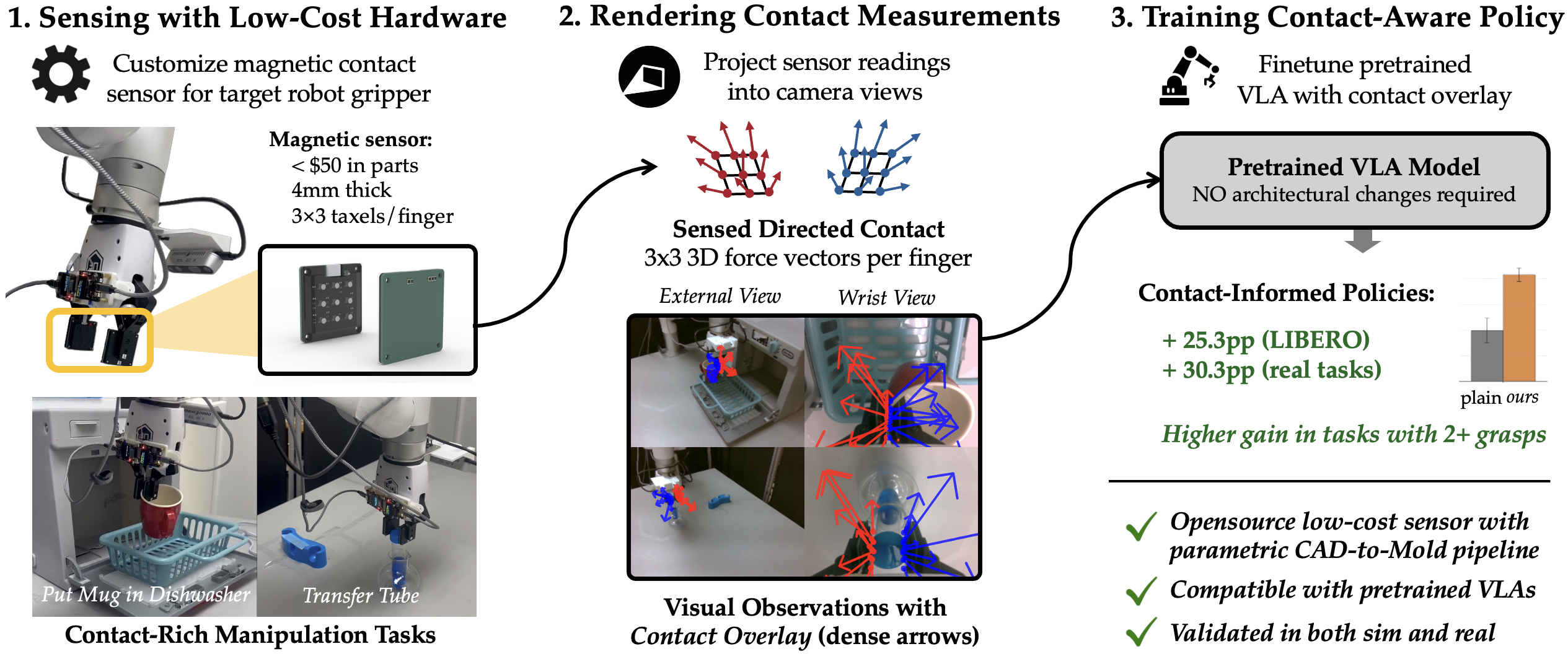
Contact measurements become colored arrows or bars in RGB observations, allowing existing image-conditioned policies to use touch without a new encoder. A low-cost magnetic sensor supplies real measurements. Two-view BC-Transformer improves by 15.7 percentage points on LIBERO; pretrained miniVLA fine-tuning improves by 25.3 points under its reported protocol. Hardware experiments favor spatially registered, per-taxel vectors, while simulated contacts favor per-finger averaging.
Keywords: imitation learning, contact-rich manipulation, tactile sensing, vision-language-action models and visual overlays.
1 Introduction
Contact can reveal a missed or insecure grasp when images are ambiguous. Visible Touch addresses sensing and integration together: cast magnetic pads provide raw contact responses, and the rendering pipeline places those responses in the visual scene. The contribution is a compatible image interface and evidence about when it helps, rather than a calibrated force estimator or a new policy architecture.
2 Related Work
Related work differs primarily in where tactile information enters a policy and how expensive or customizable the sensor is.
Contact and tactile sensing for visuomotor policies.
Earlier systems concatenate force to state, learn a tactile encoder, or construct visuotactile point clouds. Those choices can alter input dimensions or backbones. Visible Touch instead changes RGB pixels. The experiments compare particular state-vector and separate-image baselines; they do not exhaust learned fusion alternatives [19], [12].
Visual overlays as a policy interface.
Trajectory sketches, motion traces and end-effector markers already make auxiliary information visible to pretrained models. Here the signal is contact: intermittent and often hidden precisely when grasp feedback matters. Its geometric placement distinguishes the overlay from a separate contact-derived stream [7], [37].
Low-cost tactile sensors.
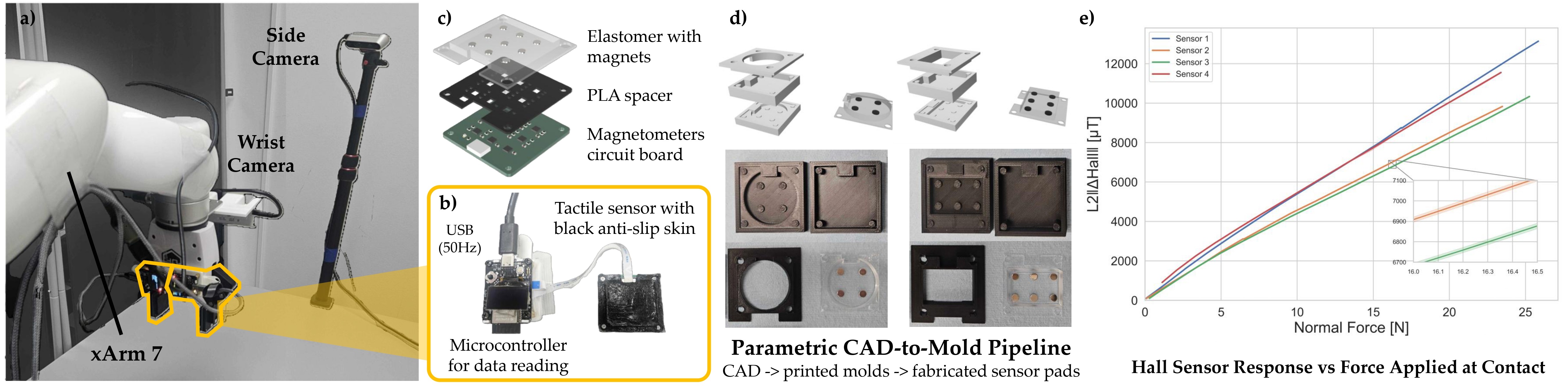
Optical sensors need dedicated optics; magnetic skins trade fabrication requirements, thickness and replaceability. The proposed molds encapsulate discrete magnets in a 4 mm cast pad, separating a replaceable contact surface from reusable electronics. Custom geometry is supported by the design pipeline, but policies are tested on only one sensor layout.
3 Visible Touch : Sensing and Rendering Contact
The system combines sensor-local three-axis measurements with a camera-aligned renderer. Simulated forces and physical magnetic deflections use the same interface, despite different units.
3.1 Overlay Representation
Forward kinematics and calibrated camera parameters locate each taxel in the current image. Rendering preserves image resolution, channels and pixel range, so the policy receives its usual RGB input.
Sensor model.
Each finger has known nominal taxel positions and three-axis signals. A signal is a simulator force vector or magnetic flux deflection, not necessarily a calibrated physical force. Per-finger means provide an aggregate alternative to individual taxels.
Projection.
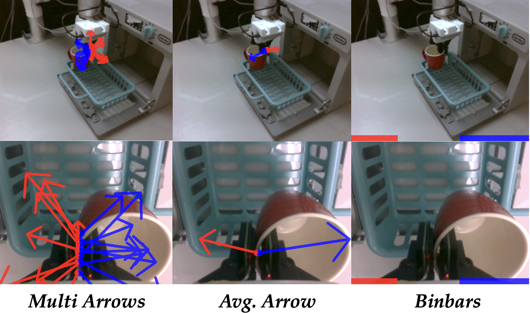
Project a taxel position and a signal-offset endpoint through the sensor-to-camera transform. Spatial and signal scales control footprint and arrow length; perspective affects the projected length. Static position markers remain when contact is zero. Finger-specific colors and alpha blending preserve the surrounding scene.
Overlay variants.
Multi-arrows retains each taxel vector; Avg. Arrow averages each finger at its center. Binbars uses aggregate magnitude at a fixed screen location, discarding contact direction and spatial registration. These variants trade information against visual clutter.
3.2 Custom Magnetic Tactile Sensor
Nine magnets in a soft silicone pad sit above nine three-axis magnetometers per finger. A microcontroller streams raw flux at 50 Hz. Printed molds, a spacer and a protective skin enable replaceable pads. The reported material cost is under $5 for the pad and under $50 including electronics; it excludes labor and fabrication equipment.
4 Experiments
Experiments examine gains across policy families, compare integration strategies, and test when task structure or overlay granularity changes the benefit.
4.1 Simulation Experiments on LIBERO
Simulation separates controlled from-scratch BC-Transformer comparisons from pretrained miniVLA experiments. The two protocols have different training budgets and uncertainty reporting.
Setup.
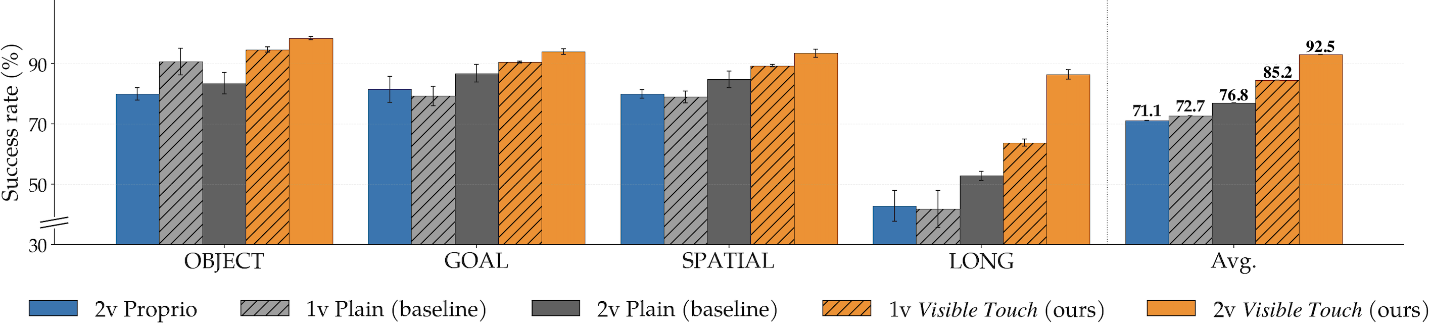
MuJoCo finger contacts provide simulated signals. BC-Transformer trains multitask models for three seeds, evaluating final checkpoints with 20 rollouts per task. Plain inputs have RGB and 8-D state; Proprio adds a 12-D aggregate wrench; Visible Touch adds image overlays. Proprio and overlays are not exactly information-matched. One- and two-camera settings are tested [17].
| Pretraining | Fine-tuning | |||||
|---|---|---|---|---|---|---|
| LIBERO_90 | OBJECT | GOAL | SPATIAL | LONG | Avg. | |
| Baseline | 48.3% | 51.0% | 48.5% | 71.5% | 32.5% | 50.9% |
| Visible Touch | 63.2% | % | % | % | % | 76.2% |
Q1: Overlays consistently improve performance and transfer across architectures.
Two-view BC-Transformer improves from 76.8% to 92.5% average success; one-view gains 12.5 points. LONG gains 33.7 points in two views. miniVLA pretraining yields 63.2% versus 48.3% under the stated reevaluation, while fine-tuning averages 76.2% versus 50.9%; its baseline and overlay seed protocols differ.
Q2: Image-space delivery outperforms a compact state-vector baseline and an information-matched separate-stream alternative.
Visible Touch exceeds the 12-D Proprio baseline by 21.4 points on average; Proprio itself trails plain two-view inputs by 5.7 points. This establishes a difference for the tested compact concatenation, not a general inability to use tactile features outside images.
| Visible Touch variant | OBJECT | GOAL | SPATIAL | LONG | Avg. |
|---|---|---|---|---|---|
| Multi-arrows | |||||
| Avg. Arrow | |||||
| Binbars |
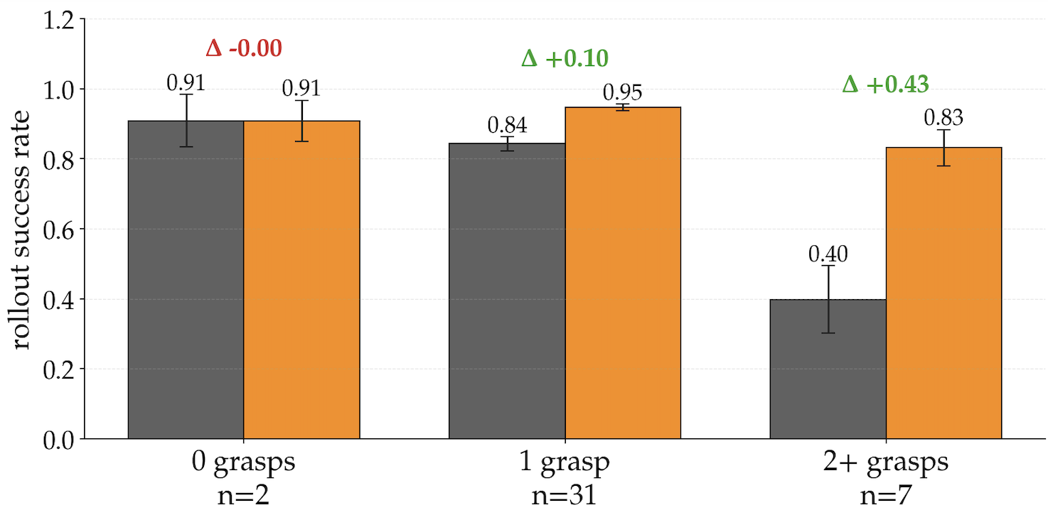
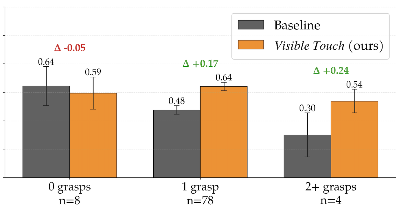
Q3a: Overlay benefit scales with task headroom and grasp structure (across architectures).
Raw gains correlate strongly with available headroom (r = 0.924), and multigrasp groups show large gains. After controlling for headroom, contact onsets and trajectory length have negative partial correlations with gain. Thus the positive raw grasp-structure association does not establish that more contact events independently cause larger improvements.
Q3b: Overlay granularity has a non-monotonic optimum.
Avg. Arrow averages 92.5%, versus 91.0% for Binbars and 88.1% for Multi-arrows. Finer simulated contact locations can introduce clutter or inconsistency; the proposed explanation is tested indirectly and reverses with fixed physical taxels.
4.2 Real-World Validation with 𝝅 0.5
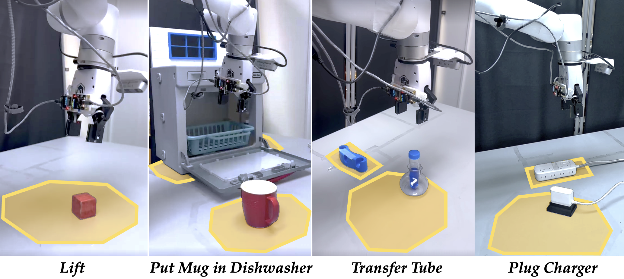
The hardware study adapts π0.5 to four contact-rich tasks using identical underlying demonstrations across eight input conditions.
Setup.
An xArm7 uses external and wrist cameras plus two 3×3 magnetic pads. Eight conditions include plain RGB, separate Tac-View, position-only markers, two binary-contact variants and three full-signal overlays. Each has 30 trials per task. The +30.3-point result macro-averages subtask gains within each task before averaging tasks; final-stage counts separately measure complete execution [24].
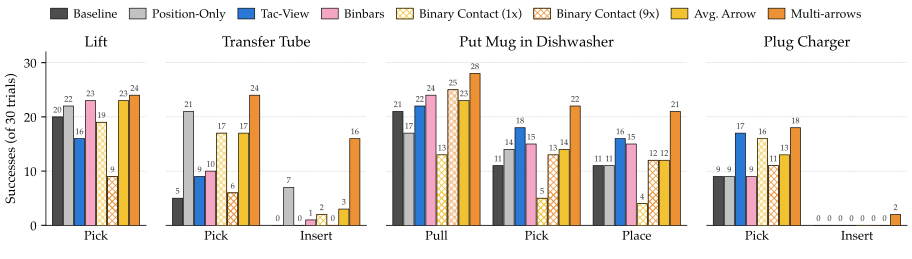
Q1: Visible Touch transfers to real-world contact-rich manipulation.
Multi-arrows improves every reported stage. Complete-task counts rise from 20 to 24/30 for Lift, 0 to 16/30 for Tube, 11 to 21/30 for Dishwasher and 0 to 2/30 for Charger. Averaging these final-stage rates gives a 26.7-point gain (calculated from Table 15), while the paper's subtask-weighted aggregate is 30.3 points. Charger insertion remains difficult.
Component ablations further isolate the source of these gains.
Position markers alone improve several stages, so localization explains part of the effect. Binary contact is weaker than full-vector counterparts on difficult tasks, supporting a role for direction and magnitude beyond knowing that contact occurred.
Encoder-architecture robustness.
Benefits appear with convolutional and transformer visual encoders across three policy families. Because the study changes more than the encoder between families, this is transfer evidence rather than a controlled causal comparison of encoder architectures.
Q2: Image-space overlay outperforms separate-stream tactile rendering.
Tac-View renders the same per-taxel arrows in a separate camera slot. It helps several tasks but loses to Multi-arrows on every stage, notably Tube pick (9 versus 24/30) and insert (0 versus 16/30). Coarse overlays do not universally beat Tac-View, making spatial detail important to this comparison.
Q3b: Optimal granularity reverses in real-world.
Physical Multi-arrows is strongest, unlike the simulation result. The authors attribute this to fixed taxel locations versus moving collision points. Binary nine-taxel feedback still performs poorly, so spatial granularity alone is insufficient; the signal-consistency explanation remains a hypothesis.
5 Conclusion
Rendering touch into RGB is a practical interface for adapting existing image policies. The results favor this interface under the tested data, sensor and training conditions, with task-dependent choices about signal detail.
Limitations.
Only one compact state-vector baseline, one robot, four hardware tasks and one 3×3 sensor geometry are evaluated. Learned tactile fusion, other morphologies, deformable objects and unstructured environments remain open. Mold customization does not yet demonstrate policy transfer between sensor geometries.
Acknowledgments
The authors acknowledge institutional and computing support from UCLA and discussions with the Robot Intelligence Laboratory and RoMeLa.
Appendix
The appendices retain the projection equations, full sensor recipe and characterization, seed-level simulation results, training details and hardware evaluation protocol.
Appendix A Projection Pipeline Derivation
The four equations specify the kinematic transforms, signal-offset endpoint and pinhole projection used for overlay registration.
Kinematic chain.
Compose fingertip forward kinematics with the fixed finger-to-sensor transform. The external camera has a fixed calibration; the wrist camera transform updates with joint configuration. Frame direction matters when composing the inverse wrist pose.
Equations 1–2
| (1) |
| (2) |
Arrow tail and tip in camera frame.
Scale taxel position by the footprint factor and add a scaled local signal for the arrow tip; use zero offset for its tail. Transform both to the camera frame. Sensor axes therefore rotate with the gripper rather than remaining fixed on screen.
Equation 3
| (3) |
Pinhole projection.
Pinhole projection divides camera-frame coordinates by depth and applies focal lengths and principal point. Identical signal magnitudes can produce different pixel lengths through perspective.
Equation 4
| (4) |
Per-variant rendering.
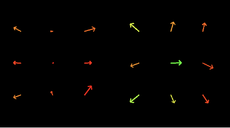
Multi-arrows projects each element; Avg. Arrow projects a per-finger mean; Binbars displays mean magnitude at a fixed location. Overlays use cyan/blue and magenta/red for finger identity. Tac-View instead colors arrows by normalized normal-axis readings from green to red.
Appendix B Tactile Sensor Hardware Details
The hardware appendix provides costs, a reproducible casting procedure and measurements of response, consistency, hysteresis and drift.
B.1 Bill of Materials
Table 3 separates the replaceable pad subtotal ($3.62) from approximately $41 in reusable electronics. Prices depend on order size and omit equipment and labor.
| Component | Spec | Qty | Unit price | Subtotal |
|---|---|---|---|---|
| Sensor pad (consumable) | ||||
| XP-565 silicone elastomer | 10:1 base/activator | 10 g | $0.05/g | $0.50 |
| Neodymium magnets | 2 mm 1 mm | 9 | $0.07/ea | $0.63 |
| PLA filament (molds + spacer) | — | 20 g | $0.013/g | $0.26 |
| Loctite SF 770 | — | 1 ml | $0.50/ml | $0.50 |
| Loctite 406 | — | 0.5 ml | $1.65/ml | $0.83 |
| Anti-slip skin | — | 1 ml | $0.10/ml | $0.10 |
| Machine screws | M26 | 4 | $0.20/ea | $0.80 |
| Sensor pad subtotal | $3.62 | |||
| PCB electronics (reusable) | ||||
| Magnetometer array PCB | Allegro A31031 | 1 | $20 | $20 |
| Microcontroller board | ESP32-based [28] | 1 | $20 | $20 |
| Flexible flat cable | 10 pin 0.5 mm, 15 mm length | 1 | $1/ea | $1 |
| Electronics subtotal | $41 | |||
| Total (fully assembled) | $50 | |||
B.2 Fabrication Procedure
Fabrication takes about 48 elapsed hours excluding printing, largely for silicone and adhesive curing. The original eight-panel fabrication figure is retained.
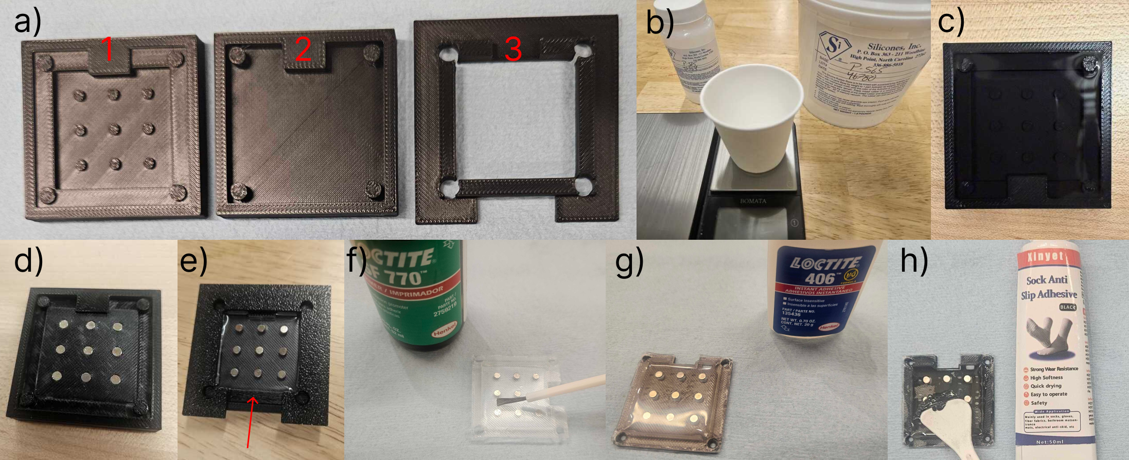
Step 1: Mold and spacer preparation (Fig. 8 a).
Print the first mold with blind magnet cavities, two split secondary-mold halves and a spacer fitted to the circuit board. The split mold permits insertion of the partially cured pad.
Step 2: Elastomer preparation and first pour (Fig. 8 b–c).
Mix silicone at 10:1 by weight (6 g base, 0.6 g activator), degas for 20 minutes at approximately 0.6 bar below ambient, then partially cure the first pour for 6.5 hours. The pad must hold shape while remaining able to bond to the next layer.
Step 3: Magnet encapsulation and second pour (Fig. 8 d–e).
Prepare a second 4 g + 0.4 g batch. Transfer the pad, seat nine 2 mm-diameter by 1 mm magnets, assemble the secondary mold, fill and cure for 16 hours. The second layer encapsulates the magnets at the specified layout.
Step 4: Adhesion treatment and bonding to spacer (Fig. 8 f–g).
Prime the cured pad with the specified silicone adhesion promoter, allow one minute to flash off, then bond it to the spacer with cyanoacrylate and allow a one-minute initial set.
Step 5: Protective skin application and final assembly (Fig. 8 h).
Apply anti-slip skin, allow 24 hours for adhesive curing and fasten the pad, circuit board and finger mount with screws. The released parametric molds and board layout support reproducing or redesigning the hardware; learned policy portability is not evaluated.
B.3 Sensor Characterization
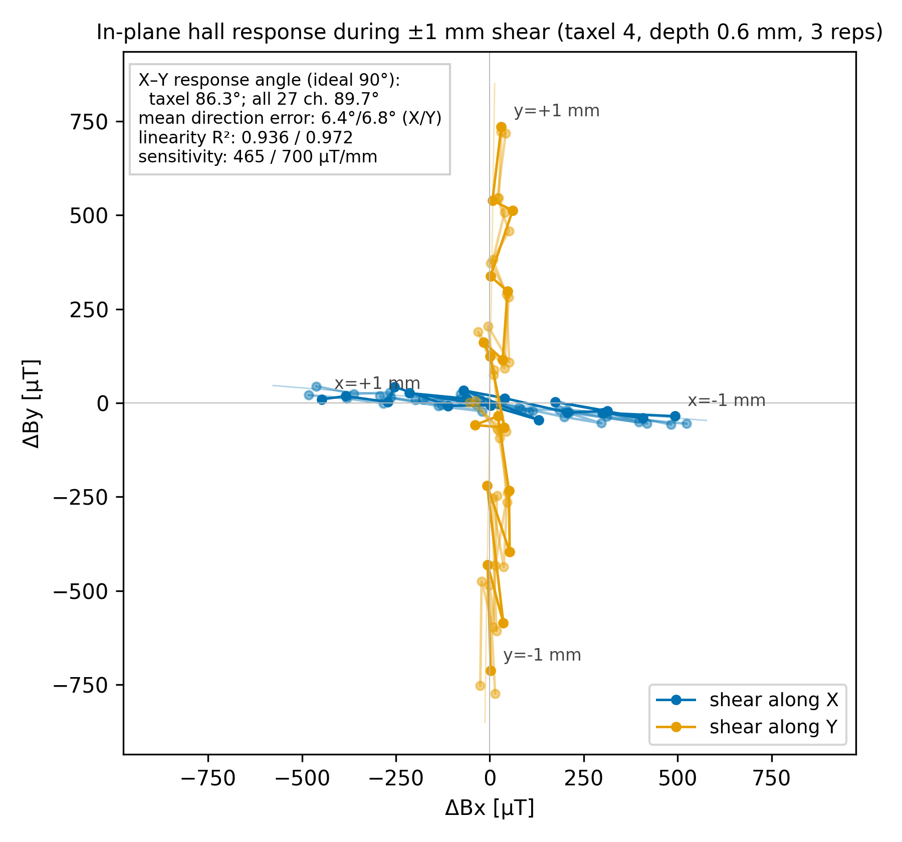
Normal-force repeatability uses four independently cast sensors made by one operator with the same geometry. Shear, hysteresis and drift use one representative unit, limiting conclusions about manufacturing variability.
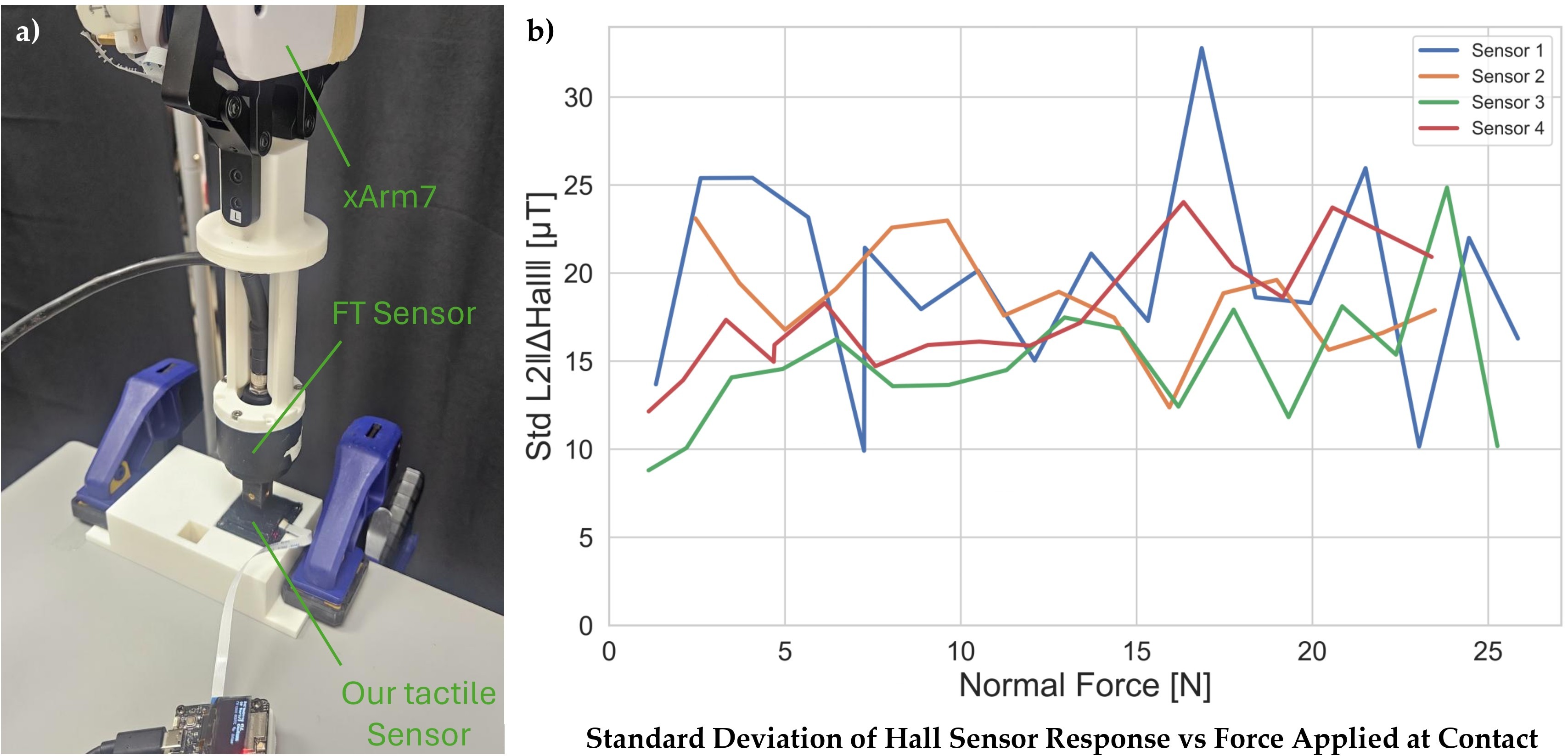
Experimental setup.
A force-torque sensor and 14×14 mm probe provide simultaneous reference forces and all nine magnetic readings during controlled normal, tangential and cyclic motion or stationary holds.
Response metrics.
Subtract each channel's pre-contact offset. Aggregate response is the Euclidean norm of all 27 corrected channels; shear analyzes in-plane channels and drift analyzes channel deviations. Magnetic response units remain microtesla, rather than force.
Normal-force response and consistency across units.
Twenty repeats at each 0.1 mm indentation step up to 1.6 mm give smooth monotonic curves and roughly 10–30 microtesla within-unit standard deviation. Between-unit response differs by about 20%. Demonstrations and normalization use the same sensor as deployment, so this is not a cross-unit policy-transfer test.
Shear response and directional accuracy.
At 0.6 mm indentation, ±1 mm tangential sweeps produce nearly orthogonal, sign-symmetric responses. Reported sensitivities are 465/700 microtesla per mm along X/Y, with R² 0.936/0.972, at most 10% cross-axis response and about 7° mean direction error under this settled protocol.
Hysteresis.
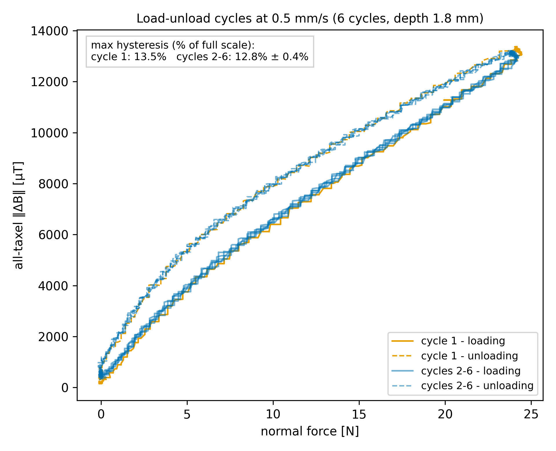
Six cycles to 24 N at 0.5 mm/s produce 12.4–13.6% full-scale loading–unloading separation. Similar loops across cycles suggest no observed conditioning drift, but the response still has measurable hysteresis and speed-dependent viscoelastic lag.
Baseline drift.
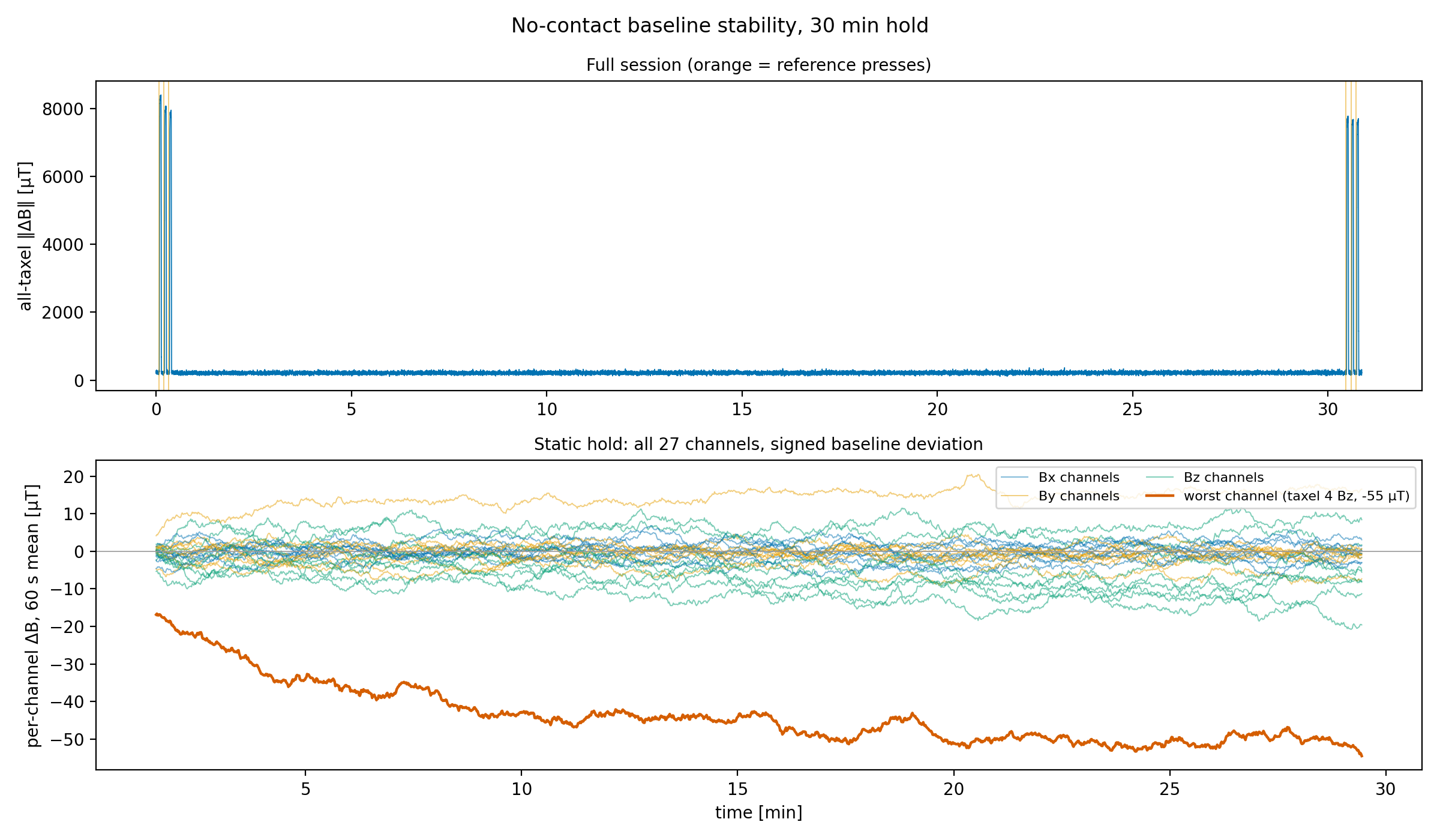
During a 30-minute hold, 26/27 channels remain within ±20 microtesla in minute averages. The largest settling excursion is −55 microtesla, about 0.7% of a typical press signal; reference presses differ by up to 5.2%. Episode offsets remove slow shifts. A rolling median replaced serial errors in 0.04% of recorded frames.
Appendix C Details of BC Transformer on LIBERO
This appendix records the BC-Transformer configuration and all aggregate, task-level and seed-level comparisons.
C.1 BC-Transformer Details
The LIBERO multitask baseline uses a randomly initialized ResNet-18, language-conditioned features, four transformer layers and a Gaussian-mixture action head. Training runs 20 epochs at batch 32 with 128×128 images and ten-frame context; Table 4 preserves the complete configuration.
| Component / Hyperparameter | Value |
|---|---|
| Architecture | |
| Visual backbone | ResNet-18 (random init, remove_layer_num=4, no stride change) |
| Language fusion | FiLM conditioning on visual features |
| Language encoder | 1-layer MLP (input , hidden , output ) |
| Transformer layers | |
| Hidden / embed dimension | (token embed); MLP hidden |
| Attention heads | (per-head dim ) |
| Action head | GMM head, MLP layers, hidden , modes, softplus, min_std |
| Proprio inputs | gripper_states, joint_states (eye_in_hand + agentview RGB) |
| Optimization | |
| Optimizer | AdamW (, ) |
| Learning rate | (cosine annealing to ) |
| Weight decay | |
| Dropout | (transformer) |
| Gradient clipping | |
| Batch size | |
| Training epochs | |
| Sequence & action | |
| Sequence length (context) | frames (transformer_max_seq_len, seq_len) |
| Frame stack | |
| Action chunking | None (single-step action prediction) |
| Action scale | |
| Image resolution | |
| Data augmentation | batch-wise color jitter + translation aug |
| Lifelong configuration | |
| lifelong.algo | Multitask (all tasks jointly via learn_all_tasks) |
| eval_in_train | false |
C.2 LIBERO Main Results
Table 5 reports three-seed means and standard deviations for both camera configurations and the compact contact-state baseline.
The overlay benefit grows with task difficulty.
Two-view gains are about 6–15 points on OBJECT, GOAL and SPATIAL, versus 33.7 on LONG. Low baseline performance leaves more headroom, so the larger LONG gain should be interpreted alongside its starting success rate.
Overlays stabilize as well as improve.
The median cross-seed standard deviation is 2.4 points for Visible Touch, versus 4.1 for plain and 3.2 for Proprio. Three seeds provide evidence of reduced variability in this setting, not a broad stability guarantee.
Proprio underperforms plain on every suite.
The Proprio baseline trails plain two-view RGB by 2.8–10.0 points across suites, averaging 71.1% versus 76.8%. The comparison isolates this particular compact input implementation; it does not rule out learned encoders or other feature fusion.
The wrist camera helps Visible Touch universally but hurts plain on OBJECT.
Adding a wrist camera improves plain average success by 4.1 points but reduces OBJECT by 7.9. It improves Visible Touch on all four suites, averaging 7.3 points. Overlay and camera benefits therefore interact with training stability and task content.
C.3 Per Task Analysis on LIBERO
Per-task results identify large rescue cases and the high-variance task behind the unusual OBJECT camera regression.
Rescue Outliers
The largest gains include butter-to-basket (+50 points), wine-to-top-of-cabinet (+17), a ramekin-to-plate task (+32) and a cheese-and-butter sequence (+87). The authors connect these cases to visually ambiguous or precarious grasps.
| Suite | Task | Plain 2v | Visible Touch 2v | |
|---|---|---|---|---|
| OBJECT | butter basket | |||
| GOAL | wine top of cabinet | |||
| SPATIAL | bowl on ramekin plate | |||
| LONG | cheese + butter basket |
OBJECT 2-View Training Instability
One butter-to-basket task largely drives plain two-view OBJECT instability. Excluding it raises the remaining-task average to 87%. The proposed undertraining explanation is not a controlled diagnosis; the original 20-epoch result is retained rather than selecting a favorable checkpoint.
C.4 Task-Level Correlation Analysis
The analysis measures associations across 40 tasks and explicitly controls for the limited improvement possible on already successful baselines.
Task properties.
Task features are baseline headroom, median gripper-close count, mean trajectory length, fraction of contact steps and mean contact-onset count, derived from demonstrations and simulator contact extraction.
Outcome variable.
The outcome is the per-task difference between seed-averaged Visible Touch and plain two-view success rates.
Raw and partial correlations.
Pearson correlations summarize raw associations; partial correlations regress headroom out of both variables. After this adjustment, grasp count and contact fraction are not significant, while contact onsets and trajectory length retain negative correlations. These observational relationships are not causal tests.
| Raw Pearson | Partial (controlling for headroom) | |||
|---|---|---|---|---|
| Feature | ||||
| Headroom | — | — | ||
| #grasps | ||||
| Trajectory length | ||||
| %contact | ||||
| #contact onsets | ||||
C.5 Additional Comparisons
Additional tables separate camera effects from seed variation.
C.5.1 Effect of Camera Configuration on Plain Baseline
The wrist camera improves plain GOAL by 7.5 points, SPATIAL by 5.8 and LONG by 11.0, while OBJECT falls by 7.9. Visible Touch's OBJECT score reaches 98.2%, but the plain regression should remain visible when interpreting the margin.
C.5.2 Seed-Level Results
Tables 9–11 retain every training seed for plain RGB, Proprio and Visible Touch. Aggregate uncertainties are standard deviations, unlike miniVLA's reported standard errors.
| Suite | Seed 12345 | Seed 23456 | Seed 34567 | Mean | SD |
|---|---|---|---|---|---|
| OBJECT | |||||
| GOAL | |||||
| SPATIAL | |||||
| LONG |
Seed-to-seed variability.
Plain OBJECT spans 73.5–90.5% across seeds. Visible Touch has narrower spreads in all four suites (standard deviations 1.2–2.7 points); Proprio LONG remains variable at 5.1 points.
Appendix D miniVLA on LIBERO Details
miniVLA experiments include training from visual-language weights, adapting a released checkpoint, recipe comparisons and orientation checks.
D.1 miniVLA Pretraining on LIBERO_90 (Contact-Overlay)
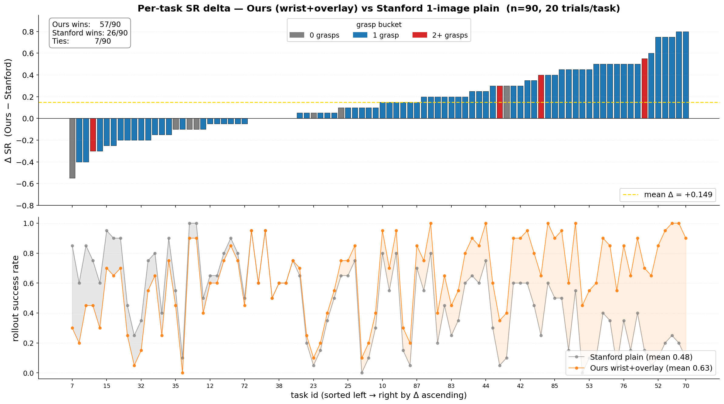
The first comparison trains contact-conditioned miniVLA on LIBERO_90 and reevaluates the released plain checkpoint. The text describes a matched single-image, no-chunking configuration, while Figure 12 labels the overlay model as wrist-plus-overlay and Stanford as one-image plain. This source inconsistency prevents assuming a fully matched camera comparison.
Backbone.
The model combines Qwen2.5-0.5B with DINOv2 and SigLIP visual features at 224 pixels. All backbone weights train, and 256 extra vocabulary tokens encode actions while leaving language tokens intact [1].
Optimization.
Training uses four GPUs, global batch 32, learning rate 2×10⁻⁵ with cosine decay, gradient checkpointing and 200,000 steps (about 11 epochs). Checkpoints save every 25,000 steps; the seed is 7.
Comparison with the released Stanford miniVLA.
The overlay model reaches 63.2% versus 48.3% across 90 tasks with 20 trials each. Its 200,000-step/global-batch-32 run differs from the released model’s 60,000-step/global-batch-256 run, schedules and hardware. Along with the camera-label discrepancy in Figure 12, these differences limit attribution to the overlay alone.
Additional comparison.
With the history-two, VQ-h8 configuration, contact fine-tuning reaches 86.3% versus 72.2% for the released checkpoint on the same evaluation pipeline (ten trials per task). The original project's 82% used another harness and is not the denominator of this 14.1-point gain.
D.2 miniVLA Fine-Tuning Details
Headline overlay results use five training seeds per suite-specific recipe; baseline and alternative-recipe results are single runs. This asymmetry limits direct statistical comparisons.
D.2.1 Recipes
Two principal recipes vary training budget and optimization, with a separate two-phase SPATIAL procedure. Table 12 keeps the recipe-specific baselines visible.
b8 1-epoch.
The exploratory recipe uses batch eight on one GPU for one epoch. Its limited budget provides a quick adaptation comparison.
DDP-4 b16 cosine.
The stronger recipe uses four GPUs with batch sixteen each, cosine decay and weight decay. It supplies the headline OBJECT, GOAL and LONG overlay results.
2-phase (SPATIAL only).
The two-phase SPATIAL recipe yields 71.5% plain and 87.0±1.8% overlay (standard error across five overlay seeds). The appendix also preserves the alternative distributed single-run result.
D.2.2 Evaluation Protocol
Both camera views use the model-appropriate orientation; overlays render at resolution 256. Headline overlay uncertainty is standard error over five seeds. Baselines are single runs, and evaluation otherwise follows the reported LIBERO rollout protocol.
D.2.3 Per-Recipe Results
The table compares every reported recipe rather than collapsing the experiment into one aggregate.
| Suite | Recipe | Baseline | Visible Touch | |
|---|---|---|---|---|
| OBJECT | b8 1-epoch | pp | ||
| OBJECT | DDP-4 b16 cosine | pp | ||
| GOAL | b8 1-epoch | pp | ||
| GOAL | DDP-4 b16 cosine | pp | ||
| SPATIAL | 2-phase | pp | ||
| SPATIAL | DDP-4 b16 cosine | pp | ||
| LONG | b8 1-epoch | pp | ||
| LONG | DDP-4 b16 cosine | pp |
Tactile gains are robust across recipes.
Headline gains over the strongest available single-run baseline are 19.6, 32.0, 15.5 and 34.1 points for OBJECT, GOAL, SPATIAL and LONG. Alternative recipes also improve, with single-run gains between 10.5 and 32.5 points.
Recipe-matched comparisons support the same trend.
Recipe-matched distributed comparisons give larger GOAL/LONG gains (43.1/40.6 points) than the headline comparison because their corresponding plain runs are weaker. Using stronger available baselines is conservative on those suites, but it does not replace multi-seed baseline uncertainty.
D.3 Image Orientation Probe
The released checkpoint expects a vertical flip, while the overlay dataset uses 180° rotation. A five-trial orientation probe succeeded only with the released model's expected flip. Per-model transforms prevent an avoidable orientation mismatch; the small probe is not a general robustness study.
Appendix E π 0.5 Fine-Tuning Details
Hardware π0.5 fine-tuning uses a common pretrained model and adapter configuration across all 32 task–input combinations.
E.1 Base Model and Variants
The roughly 2.3-billion-parameter policy starts from pi05_droid, combining a SigLIP visual encoder, Gemma language backbone and action expert. The authors chose real-data DROID initialization based on preliminary transfer behavior on their setup.
E.2 LoRA Fine-Tuning
Frozen base weights receive LoRA adapters on attention and feed-forward projections: rank/scale 16 on the backbone and 32 on the action expert. Only adapter parameters and attached scale/bias terms update; exponential moving averaging is disabled. This keeps initialization consistent across variants [11].
E.3 Observation and Action Spaces
Inputs are two 224×224 camera views plus the model's normally masked spare slot, and an eight-dimensional pose/gripper state. Seven-dimensional actions encode world-frame translation and axis-angle increments plus grasp. Ten-step chunks span one second at 10 Hz; rotational increments left-multiply the current orientation.
E.4 Hyperparameters
All variants share batch eight, AdamW, cosine learning-rate decay and a 20,000-step cap. The early-stop rule uses training-loss improvement after 3,000 steps; effective passes depend on task length and stopping time. Table 13 retains the full rule and parameters.
| Setting | Value |
|---|---|
| Base checkpoint | pi05_droid |
| Fine-tuning method | LoRA (backbone , action expert ) |
| LoRA targets | attention and FFN projections |
| Image resolution | , 3 cameras |
| Action horizon | 10 steps (1.0 s at 10 Hz) |
| Batch size | 8 |
| Optimizer | AdamW |
| Gradient clipping | global norm |
| LR schedule | cosine with linear warmup |
| warmup steps | 500 |
| peak LR | |
| decay steps | 20,000 |
| final LR | |
| EMA | disabled |
| Maximum training steps | 20,000 |
| Checkpoint interval | 2,000 steps |
| Early stopping | relative improvement in the 1000-step |
| rolling-window mean loss for two consecutive | |
| checks, after step 3,000 |
E.5 Compute and Wall-Clock
Each run is allocated four H200 GPUs, eight CPU cores and 96 GB memory with a 24-hour limit. Most stop around 5,100–7,900 steps; some reach 20,000. Allocations and limits should not be read as measured total compute consumption.
Appendix F Real-World Experiment Details
The hardware protocol documents signal normalization, demonstration filtering, reset randomization, stage scoring and retry behavior.
F.1 Hardware Setup
Subtract a no-contact baseline for each magnetometer axis, then divide by its maximum absolute value across demonstrations. Dataset scales remain fixed; resting offsets reset at each episode. Camera/sensor spatial calibration and these statistics remain necessary even though the method does not calibrate flux into force units.
F.2 Demonstration Collection
TeleDex records 100 attempted demonstrations per task with RGB, robot state, raw flux and gripper state. Input variants are generated afterward from the same recordings, avoiding separate demonstrations as a confound [25].
Episode statistics.
After filtering, 397 demonstrations remain: 100 each for Lift, Charger and Dishwasher, and 97 for Tube. Mean duration is 21.0±7.4 seconds at 10 Hz; task-level lengths and ranges remain in Table 14.
Acceptance criterion.
Acceptance requires a gripper open-to-close transition and at least five non-paused steps after trimming leading motion below 0.5 mm and 0.5°. It does not require task success, so the training data can contain imperfect executions. Three inactive Tube episodes are rejected.
| Task | Length (steps) | Duration (s) | Min/Max (steps) | |
|---|---|---|---|---|
| cube | 100 | 90 / 972 | ||
| tube | 97 | 166 / 238 | ||
| charger | 100 | 182 / 329 | ||
| dishwasher | 100 | 236 / 554 | ||
| All | 397 | 90 / 972 |
F.3 Evaluation Protocol
Every condition receives 30 trials per task with objects uniformly sampled within marked reset regions. Subtasks and final-stage completion are reported separately, with exact counts in Table 15.
| Lift | Transfer Tube | Put Mug in Dishwasher | Plug Charger | ||||||
| Method | Pick | Pick | Insert | Pull | Pick | Place | Pick | Insert | |
| Baseline | 20/30 | 5/30 | 0/30 | 21/30 | 11/30 | 11/30 | 9/30 | 0/30 | |
| Tac-View | 16/30 | 9/30 | 0/30 | 22/30 | 18/30 | 16/30 | 17/30 | 0/30 | |
| Position-Only | 22/30 | 21/30 | 7/30 | 17/30 | 14/30 | 11/30 | 9/30 | 0/30 | |
| Visible Touch | Binbars | 23/30 | 10/30 | 1/30 | 24/30 | 15/30 | 15/30 | 9/30 | 0/30 |
| Binary Contact (1x) | 19/30 | 17/30 | 2/30 | 13/30 | 5/30 | 4/30 | 16/30 | 0/30 | |
| Avg. Arrow | 23/30 | 17/30 | 3/30 | 23/30 | 14/30 | 12/30 | 13/30 | 0/30 | |
| Binary Contact (9x) | 9/30 | 6/30 | 0/30 | 25/30 | 13/30 | 12/30 | 11/30 | 0/30 | |
| Multi-arrows | 24/30 | 24/30 | 16/30 | 28/30 | 22/30 | 21/30 | 18/30 | 2/30 | |
Step budget and action scale.
Step limits are 150 for Lift, 400 for Tube and 600 for Dishwasher/Charger. Action scales are respectively 0.8, 0.4, 0.8 and 0.6. These budgets permit different numbers of recovery attempts across tasks.
| Task | Step budget | Action scale |
|---|---|---|
| Lift | 150 | 0.8 |
| Transfer Tube | 400 | 0.4 |
| Put Mug in Dishwasher | 600 | 0.8 |
| Plug Charger | 600 | 0.6 |
Per-stage success criteria.
Stage criteria require lifting or stable holding, the rack reaching its target, seating the mug or tube, and fully seating the plug. The protocol terminates trials on a reported collision failure. Intermediate success alone is not credited as complete-task success.
Retry behavior.
Policies may retry within the budget. Tube is the qualitative exception: tactile variants retry missed grasps, while vision-only execution can wait until timeout. The authors attribute this to transparent-object ambiguity; the observation supports recovery behavior but does not independently prove the proposed perceptual mechanism.