Overview
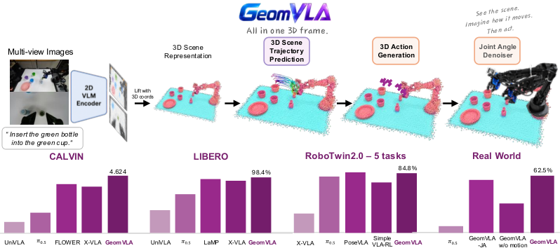
GeomVLA connects language-conditioned scene geometry, latent future motion, and action generation in one metric coordinate frame. The opening figure illustrates the shared representation.
At a glance
GeomVLA lifts vision-language features into 3D, learns future point-motion representations, and conditions a geometric action denoiser on them. With benchmark demonstrations and no robot-action pretraining, it reaches 4.624 completed tasks on CALVIN, 98.4% on LIBERO, and 62.5% mean success across eight real tasks. Ablations support consistent geometry and learned motion features, with added inference cost.
1 Introduction
Image-plane reasoning can disconnect scene understanding from metric robot actions. GeomVLA represents the current scene, future point motion, and end-effector actions in the robot base frame so spatial relations remain consistent across perception and control.
Related references: [1], [2], [3], [4], [5], [6], [7], [8], [9], [10], [11], [12], [13], [14], [15], [16], [17], [18], [19], [20], [21], [22], [23], [24], [25], [26], [27], [28], [29].
2 Related Work
Prior 3D policies ground actions geometrically, while motion-guided policies predict images, tracks, or latent futures. GeomVLA couples both through task-conditioned 3D motion features and geometry-aware action attention.
Related references: [10], [9], [30], [11], [31], [32], [33], [34], [14], [15], [18], [17], [35], [36], [37], [38], [39], [40], [41], [20], [42], [43], [44], [21], [26], [22], [24], [45], [46], [25], [47], [23], [48], [49], [50], [51], [52], [53], [54].
3 Method
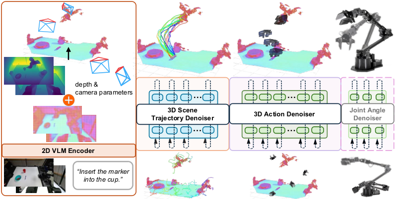
Multi-view RGB-D observations, language, and proprioception enter a three-stage pathway: lifted 3D scene features, a point-trajectory denoiser, and an action denoiser. Intermediate motion features guide actions without requiring a fully generated future trajectory.
3.1 3D Scene Features
Florence-2 encodes image patches and language. Depth and camera calibration associate each visual token with a point in the robot base frame. Proprioceptive tokens are anchored at the current end-effector pose.
Related references: [6].
3.2 3D Scene Trajectory Denoiser
A 20×20 grid supplies 400 3D anchors. A flow-matching decoder predicts displacement increments conditioned on local geometry, image features, and language. SpatialTrackerV2 supplies pseudo-labels from demonstration videos. Motion-weighted training emphasizes moving points while retaining static structure.
Equations 1–2
| (1) |
| (2) |
3.3 3D Action Denoiser
During policy inference, one trajectory-denoiser evaluation at the initial noise state supplies latent features; the model does not integrate a complete future trajectory. Temporal pooling gives one motion token per anchor, then geometry-aware attention fuses motion with scene tokens. A separate flow denoiser predicts end-effector translation and rotation, plus binary gripper state.
Equations 3–6
| (3) | ||||
| (4) | ||||
| (5) |
| (6) |
3D reasoning for joint-space control.
A downstream joint-angle denoiser can use the same scene-motion and intermediate end-effector features to produce executable joint commands, allowing the geometric representation to be tested under a matched output space.
3.4 Training
First, train the trajectory denoiser on point-track pseudo-labels with the vision-language backbone frozen. Second, jointly fine-tune the backbone, motion module, and action denoiser using only the action loss. Initialization includes pretrained Florence-2, but no robot-action pretraining.
Implementation details.
Videos are downsampled by three. Fifteen predicted displacement steps span 45 original frames; coordinates remain in the robot base frame.
Related references: [55].
4 Experiments
The evaluation tests motion supervision, shared geometry, simulation performance, and transfer to tabletop manipulation.
4.1 Simulation Experiments
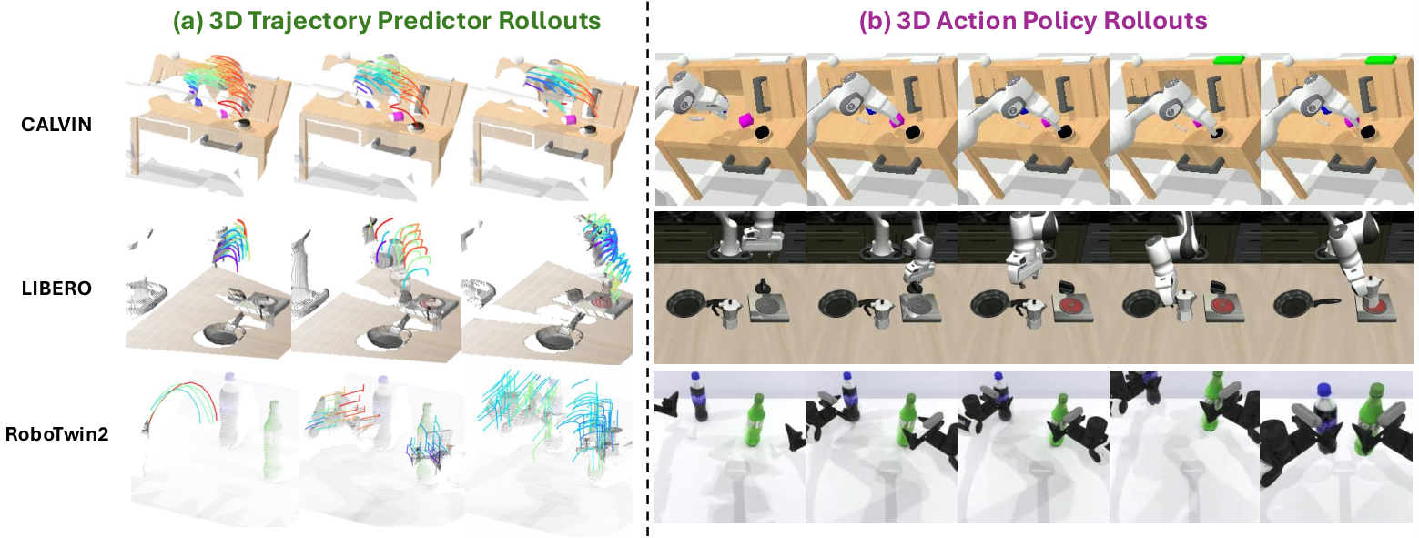
Simulation covers CALVIN, LIBERO, and RoboTwin2.0. Full GeomVLA and the main π0.5 baseline train on all fifty RoboTwin tasks; several variants train only on a five-task subset. Comparisons across those training sets are not fully controlled ablations.
Related references: [56], [27], [28], [29].
| Method | Pretrained | Params | CALVIN | LIBERO | RoboTwin2.0 | |||||||||
| ABC_D | Spatial | Object | Goal | Long | Avg. | a | b | c | d | e | Avg. | |||
| 3D VLA | ||||||||||||||
| 3D-VLA | Yes | – | 0.707 | – | – | – | – | – | – | – | – | – | – | – |
| SpatialVLA | Yes | 4B | – | 88.2 | 89.9 | 78.6 | 55.5 | 78.1 | – | – | – | – | – | – |
| 4D-VLA | Yes | 4B+ | – | 88.9 | 95.2 | 90.0 | 79.1 | 88.6 | – | – | – | – | – | – |
| PoseVLA | Yes | 3B+ | – | 96.5 | 98.0 | 97.1 | 92.4 | 96.0 | 93.5 | 87.0 | 58.0 | 93.0 | 96.5 | 85.6 |
| Video/Motion-Guided | ||||||||||||||
| TraceVLA | Yes | 7B | – | 84.6 | 85.2 | 75.1 | 54.1 | 74.8 | – | – | – | – | – | – |
| mimic-video | Yes | 2B+ | – | 94.2 | 96.8 | 90.6 | – | 93.9 | – | – | – | – | – | – |
| WorldVLA | No | 7B | – | 87.6 | 96.2 | 83.4 | 60.0 | 81.8 | – | – | – | – | – | – |
| UniVLA | Yes | 7B | 3.801 | 96.5 | 96.8 | 95.6 | 92.0 | 95.2 | – | – | – | – | – | – |
| CoT-VLA | Yes | 7B | – | 87.5 | 91.6 | 87.6 | 69.0 | 81.1 | – | – | – | – | – | – |
| FlowVLA | Yes | 8.5B | – | 93.2 | 95.0 | 91.6 | 72.6 | 88.1 | – | – | – | – | – | – |
| LaMP | Yes | 5B | – | 99.4 | 99.8 | 97.4 | 96.7 | 98.3 | – | – | – | – | – | – |
| RoboFlow4D | Yes | 0.76B+ | – | 90.2 | 97.0 | 88.4 | 75.2 | 87.7 | – | – | – | – | – | – |
| Others | ||||||||||||||
| Yes | 3B+ | 3.964 | 98.8 | 98.2 | 98.0 | 92.4 | 96.8 | 82.0 | 94.0 | 90.0 | 47.0 | 93.0 | 81.2 | |
| OpenVLA-OFT | Yes | 7B | 4.279 | 97.6 | 98.4 | 97.9 | 94.5 | 97.1 | 28.1 | 29.7 | 28.1 | 45.3 | 40.6 | 34.4 |
| FLOWER | Yes | 0.95B | 4.480 | 97.2 | 99.3 | 96.9 | 94.5 | 97.0 | – | – | – | – | – | – |
| SimpleVLA-RL | Yes | 7B | – | 99.4 | 99.1 | 99.2 | 98.5 | 99.1 | 87.5 | 68.3 | 61.2 | 89.2 | 75.8 | 76.4 |
| X-VLA | Yes | 0.9B | 4.430 | 98.2 | 98.6 | 97.8 | 97.6 | 98.1 | 48.0 | 28.5 | 47.0 | 69.0 | 46.5 | 47.8 |
| 2D-JA | No | 1B | 4.195 | – | – | – | – | – | 39.0 | 77.0 | 88.0 | 74.0 | 53.0 | 66.2 |
| GeomVLA-JA | No | 1.3B | 4.508 | – | – | – | – | – | 71.0 | 75.0 | 91.0 | 95.0 | 76.0 | 81.6 |
| GeomVLA w/o motion | No | 1.2B | 4.508 | 94.8 | 99.2 | 88.2 | 91.8 | 93.5 | 45.0 | 96.0 | 83.0 | 83.0 | 43.0 | 70.0 |
| GeomVLA | No | 1.2B | 4.624 | 98.6 | 99.8 | 97.6 | 97.6 | 98.4 | 89.0 | 98.0 | 99.0 | 55.0 | 83.0 | 84.8 |
Results.
GeomVLA scores 4.624 on CALVIN and 98.4% on LIBERO. Across all fifty RoboTwin tasks, Easy/Hard success is 78.6%/76.2% versus 75.9%/75.7% for fully fine-tuned π0.5. The five-task results in the main table should be distinguished from this full-benchmark comparison.
Related references: [3], [57], [7], [56], [8], [14], [15], [16], [58], [22], [59], [20], [41], [60], [21], [46], [25].
4.2 Ablation Studies
On CALVIN, adding motion raises the 3D policy from 4.508 to 4.624. Fully denoised trajectories, late latents, or encoder features perform worse than early motion latents. Mixing 2D motion with 3D actions drops performance to 4.085. Applying one shared rigid transform preserves most performance (4.596), suggesting consistency matters more than the particular coordinate frame.
| Variant | Description | Perf. |
| GeomVLA w/o motion | Removes the 3D Scene Trajectory Denoiser. | 4.508 |
| 2DGeomVLA w/o motion | Uses a 2D image-based policy without future-motion reasoning. | 4.411 |
| 2DGeomVLA | Uses 2D future-motion reasoning with a 2D action denoiser. | 4.437 |
| 2DGeomVLA LaMP-style | Uses pixel coordinates and metric depth for scene motion. | 4.462 |
| GeomVLA w/ 2D motion | Uses image-space future motion with the 3D action denoiser. | 4.085 |
| GeomVLA w/ denoised trace | Conditions action denoising on the fully denoised 3D trajectory. | 4.047 |
| GeomVLA w/ denoised latent | Conditions action denoising on the fully denoised motion latent. | 4.334 |
| GeomVLA w/ partial denoising | Reads the motion latent at instead of pure noise. | 4.484 |
| GeomVLA encoder-only | Uses only the scene trajectory encoder, without velocity prediction. | 4.443 |
| GeomVLA w/ arbitrary frame | Expresses scene, motion, and action in one arbitrary rigid frame. | 4.596 |
| GeomVLA | Unifies scene, future motion, and action in a shared 3D frame. | 4.624 |
4.3 Real-World Experiments
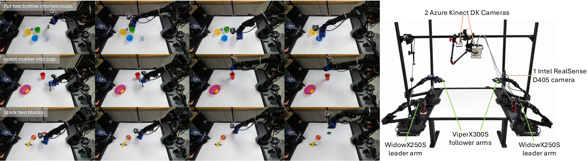
Real-world evaluation uses a single follower arm on an ALOHA2 platform.
Setup.
Teleoperation provides demonstrations. Two elevated depth cameras and a wrist camera observe the tabletop workspace.
Tasks.
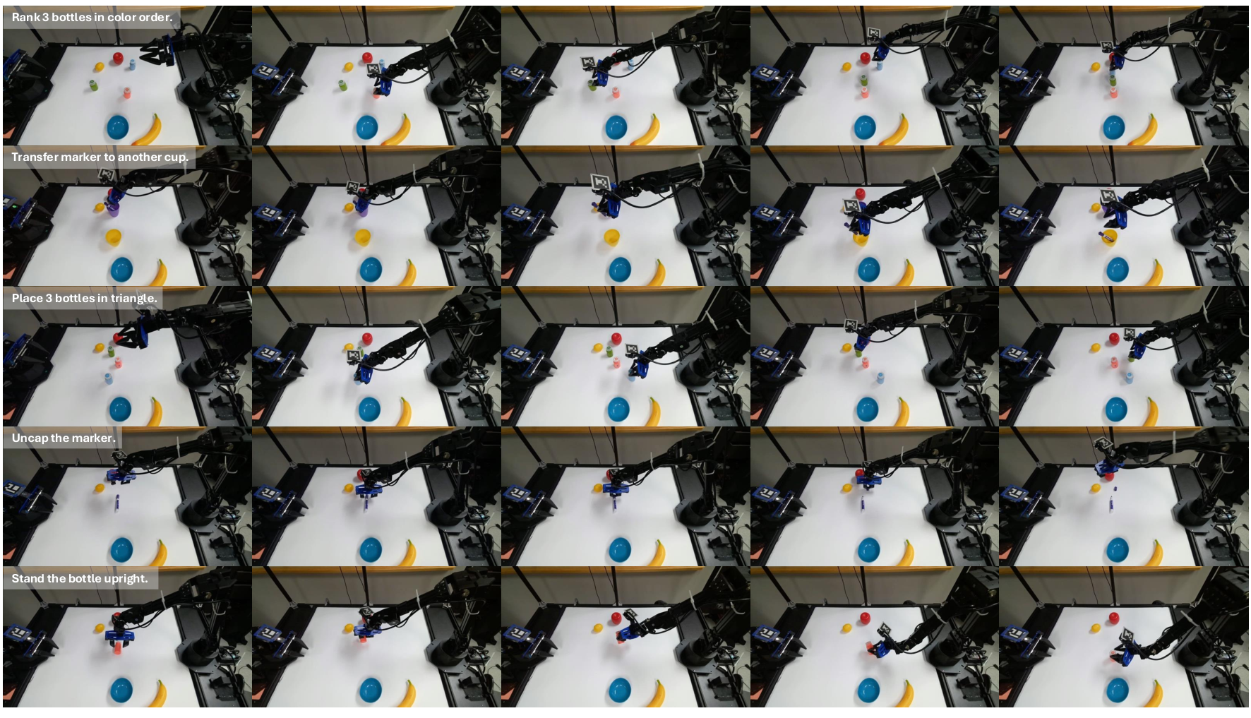
Eight tasks cover insertion, stacking, bottle placement, reorientation, transfer, uncapping, color order, and triangular arrangement. Three use fifty demonstrations each and five use twenty. Each variant trains one multi-task policy on the same demonstrations; the main π0.5 comparison additionally differs in pretraining and action parameterization.
Results.
With twenty evaluations per task, GeomVLA averages 62.5% success, beats its no-motion version on every task, and exceeds π0.5 on seven of eight. Color ordering remains difficult. Illustrated recoveries are qualitative examples, not separately quantified robustness tests.
| Task | 2D-JA | GeomVLA-JA | GeomVLA w/o motion | GeomVLA | |
| Insert marker† | 9/20 | 3/20 | 13/20 | 3/20 | 5/20 |
| Stack blocks† | 2/20 | 9/20 | 17/20 | 15/20 | 19/20 |
| Place bottles† | 10/20 | 16/20 | 16/20 | 14/20 | 17/20 |
| Stand bottle | 7/20 | 6/20 | 13/20 | 13/20 | 17/20 |
| Transfer marker | 2/20 | 0/20 | 13/20 | 10/20 | 12/20 |
| Uncap marker | 15/20 | 12/20 | 18/20 | 15/20 | 20/20 |
| Rank by color | 0/20 | 0/20 | 1/20 | 0/20 | 2/20 |
| Place in triangle | 2/20 | 0/20 | 4/20 | 1/20 | 8/20 |
| Average | 29.4% | 28.8% | 59.4% | 44.4% | 62.5% |
4.4 3D Reasoning for Joint-Angle Robot Control
GeomVLA-JA and 2D-JA share the backbone, joint-angle output head, and training data, helping isolate the representation benefit from the choice of output commands.
Results.
GeomVLA-JA exceeds 2D-JA on CALVIN (4.508 versus 4.195), the five-task RoboTwin subset (81.6% versus 66.2%), and real tasks (59.4% versus 28.8%). It performs particularly well on marker insertion: 13/20 successes versus 5/20 for the Cartesian model.
5 Limitations
The method depends on accurate depth and calibration, uses benchmark-scale demonstrations, and has not established broad cross-embodiment generalization. Its latent motion representation is not explicit verbal or hierarchical reasoning. Adding the motion pathway increases inference time.
6 Conclusion
A shared 3D representation improves the tested policies across Cartesian and joint-angle outputs. Learned early motion features appear more useful for action generation than fully reconstructed trajectories.
Appendix
The appendix retains configurations, complete RoboTwin results, stability checks, motion analyses, and detailed task descriptions.
Model configurations and compute.
Second-stage training takes about fifteen hours on four L40S GPUs for CALVIN, 25 hours on eight A100s for LIBERO, and 48 hours on eight A100s for the five-task RoboTwin setting. Table 4 records benchmark-specific architecture and optimization choices.
Lifting 2D VLM features into 3D.
Bilinearly interpolated depth at each patch center, camera intrinsics, and extrinsics lift image tokens into metric 3D positions.
3D scene trajectory encoder.
Local attention over a fixed nearest-neighbor graph combines centered coordinates and semantic descriptors. Relative-position biases preserve local geometry; global visual and language tokens condition the decoder.
Equations 7–9
| (7) |
| (8) |
| (9) |
3D scene trajectory decoder.
The trajectory decoder alternates spatial attention over Morton-ordered windows, temporal attention, and cross-attention to context. Shifted windows and axis permutations spread spatial information. Invalid or low-confidence tracks are masked, and a motion-sensitive weighting retains nonzero supervision for static points. The equations and configuration table preserve the implementation details.
Equations 10–14
| (10) |
| (11) |
| (12) |
| (13) |
| (14) |
| Module | CALVIN | LIBERO | RoboTwin2.0 – five-task ablations | Real-world | |
| Trajectory Denoiser | Hidden dim | 512 | 384 | 320 | 128 |
| Encoder layers | 6 | 6 | 6 | 4 | |
| Decoder layers | 8 | 8 | 8 | 8 | |
| Attention heads | 16 | 8 | 8 | 8 | |
| Batch size | 128 | 128 | 128 | 128 | |
| Optimizer | AdamW | AdamW | AdamW | AdamW | |
| Learning rate | 1e-4 | 1e-4 | 1e-4 | 1e-4 | |
| Iterations | 20k | 20k | 20k | 20k | |
| Action Denoiser | Hidden dim | 960 | 912 | 912 | 256 |
| Shared attention layers | 16 | 16 | 16 | 16 | |
| Attention heads | 16 | 16 | 16 | 16 | |
| Batch size | 32 | 128 | 64 | 32 | |
| Optimizer | AdamW | AdamW | AdamW | AdamW | |
| Learning rate | 2e-5 | 5e-5 | 4e-5 | 2e-5 | |
| Iterations | 50k | 80k | 300k | 50k | |
| Rotation format | Euler | Axis-angle | 6D rotation | 6D rotation | |
| Action horizon | 10 | 10 | 16 | 8 | |
| Embodiment | Single-arm | Single-arm | Bimanual | Single-arm | |
RoboTwin2.0 training protocol and full results.
Full RoboTwin training uses 27,500 demonstrations: fifty clean and five hundred randomized examples per task. Table 5 reports all fifty tasks, each evaluated in fifty Easy and fifty Hard rollouts.
| Task | GeomVLA | Task | GeomVLA | ||||||
| Easy | Hard | Easy | Hard | Easy | Hard | Easy | Hard | ||
| Adjust Bottle | 86 | 92 | 100 | 100 | Place Can Basket | 70 | 70 | 84 | 76 |
| Beat Block Hammer | 84 | 80 | 88 | 90 | Place Cans Plasticbox | 74 | 86 | 94 | 92 |
| Blocks Ranking RGB | 88 | 84 | 46 | 44 | Place Container Plate | 96 | 98 | 100 | 98 |
| Blocks Ranking Size | 52 | 38 | 24 | 32 | Place Dual Shoes | 62 | 64 | 84 | 86 |
| Click Alarmclock | 94 | 98 | 98 | 96 | Place Empty Cup | 90 | 90 | 100 | 96 |
| Click Bell | 98 | 98 | 100 | 100 | Place Fan | 88 | 84 | 88 | 86 |
| Dump Bin Bigbin | 84 | 90 | 72 | 68 | Place Mouse Pad | 44 | 36 | 88 | 90 |
| Grab Roller | 98 | 96 | 100 | 100 | Place Object Basket | 70 | 80 | 48 | 56 |
| Handover Block | 42 | 32 | 14 | 10 | Place Object Scale | 80 | 70 | 96 | 98 |
| Handover Mic | 42 | 52 | 72 | 38 | Place Object Stand | 86 | 94 | 96 | 98 |
| Hanging Mug | 16 | 14 | 6 | 4 | Place Phone Stand | 64 | 66 | 76 | 84 |
| Lift Pot | 88 | 88 | 32 | 18 | Place Shoe | 88 | 84 | 96 | 100 |
| Move Can Pot | 92 | 88 | 100 | 98 | Press Stapler | 70 | 78 | 70 | 78 |
| Move Pillbottle Pad | 80 | 88 | 96 | 94 | Put Bottles Dustbin | 34 | 38 | 34 | 18 |
| Move Playingcard Away | 74 | 76 | 98 | 96 | Put Object Cabinet | 56 | 60 | 62 | 48 |
| Move Stapler Pad | 56 | 64 | 72 | 76 | Rotate QRcode | 96 | 84 | 80 | 80 |
| Open Laptop | 90 | 92 | 94 | 92 | Scan Object | 62 | 56 | 62 | 60 |
| Open Microwave | 82 | 80 | 94 | 82 | Shake Horizontally | 96 | 98 | 100 | 100 |
| Pick Diverse Bottles | 86 | 84 | 86 | 84 | Shake Bottle | 96 | 98 | 100 | 100 |
| Pick Dual Bottles | 94 | 94 | 100 | 96 | Stack Blocks Three | 56 | 60 | 46 | 32 |
| Place A2B Left | 84 | 90 | 90 | 90 | Stack Blocks Two | 92 | 92 | 74 | 88 |
| Place A2B Right | 82 | 72 | 96 | 90 | Stack Bowls Three | 78 | 64 | 46 | 36 |
| Place Bread Basket | 74 | 68 | 86 | 86 | Stack Bowls Two | 88 | 98 | 84 | 82 |
| Place Bread Skillet | 72 | 66 | 92 | 80 | Stamp Seal | 88 | 74 | 96 | 96 |
| Place Burger Fries | 78 | 82 | 96 | 94 | Turn Switch | 56 | 58 | 72 | 72 |
Two-seed stability check on CALVIN and LIBERO.
A second seed gives CALVIN 4.609 versus 4.624 and LIBERO 98.0% versus 98.4%. This limited stability check does not quantify uncertainty for every comparison.
Evaluation of the 3D scene trajectory prediction horizon.
Increasing the trajectory horizon from fifteen to 32 raises mean error from 2.46 to 3.35 cm and endpoint error from 4.61 to 6.43 cm over the common evaluation window. CALVIN drops from 4.624 to 4.272.
| Horizon | Mean error (cm) | Endpoint error (cm) | Perf. |
| 2.46 | 4.61 | 4.624 | |
| 3.35 | 6.43 | 4.272 |
Instruction conditioning for the 3D Scene Trajectory Denoiser.
Replacing only the task instruction increases endpoint error on all three benchmarks, supporting language dependence of the learned motion predictions.
| Benchmark | Matched | Mismatched | Increase |
| CALVIN | 4.61 | 8.01 | |
| LIBERO | 9.12 | 14.56 | |
| RoboTwin2.0 | 5.77 | 7.41 |
Control for model capacity.
Replacing learned motion features with a frozen random module of equal size reduces CALVIN from 4.624 to 4.443. Added parameter count alone does not explain the measured gain.
Inference latency.
On one L40S, a ten-action chunk takes 280.0±14.0 ms with motion versus 219.0±11.3 ms without it: 27.9% overhead. The action denoiser dominates total time. Measurements cover four evaluation sequences per model after warmup.
Ablation variant descriptions.
Table 8 defines the exact changes behind each ablation, including action geometry, motion-token extraction, and coordinate alignment.
| Variant | Description |
| GeomVLA w/o motion | Removes the 3D Scene Trajectory Denoiser and directly predicts actions with the 3D action denoiser. |
| 2DGeomVLA w/o motion | Uses a 2D image-based action denoiser without future-motion reasoning. |
| 2DGeomVLA | Uses 2D future-motion reasoning with a 2D action denoiser. |
| 2DGeomVLA LaMP-style | Uses image-plane coordinates and metric depth for motion reasoning instead of metric 3D points. |
| GeomVLA w/ 2D motion | Uses image-space future motion with the 3D action denoiser. |
| GeomVLA w/ denoised trace | Conditions action denoising on the fully denoised 3D trajectory. |
| GeomVLA w/ denoised latent | Conditions action denoising on the fully denoised motion latent. |
| GeomVLA w/ partial denoising | Reads the motion latent at instead of pure noise. |
| GeomVLA encoder-only | Uses only the trajectory-denoiser encoder, without velocity prediction. |
| GeomVLA w/ arbitrary frame | Expresses scene, motion, and action in a shared arbitrary rigid frame. |
| GeomVLA | Unifies scene, future motion, and action in a shared 3D frame. |
Real-world task descriptions.
The eight tasks test precise orientation, small-object manipulation, color grounding, and sequential placement. Marker insertion, block stacking, and paired bottle placement use fifty demonstrations; the other tasks use twenty. Figure 5 shows successful rollouts with varied objects, distractors, and layouts.