Reading guide
All eight pages, four complete figures, three exact tables, eighteen numbered equation groups, four unnumbered displays, the full inverse-function theorem and forty-nine references are covered. The method differentiates a chosen analytic IK branch through an augmented forward-kinematics Jacobian. Exact local derivatives inside regular chart regions are distinct from approximate gradients outside the reachable workspace. The practical contribution is wider solver compatibility, with task-dependent accuracy, runtime and reachability assumptions.
At a glance
The paper supplies gradients for black-box analytic IK without editing generated solver code. It augments forward kinematics with the chosen redundancy coordinates, solves a linear system for derivatives, and adds approximate workspace extensions plus a log-determinant reachability surrogate. Results include agreement with bespoke autodiff on sampled reachable configurations, downstream planning comparisons, and twenty RB-Y1 box trials. The method still needs a continuous branch and well-conditioned local coordinates; arbitrary branch-switching IK is not automatically differentiable.
I Introduction
Equality constraints such as a fixed two-hand grasp confine feasible robot configurations to a lower-dimensional set. Analytic IK can chart that set, allowing optimization in smaller coordinates while checking collision and joint limits after lifting back to joint space. Generated analytic solvers often lack autodiff support. The proposed derivative interface removes that implementation barrier, while local singularities, reachable-domain boundaries and branch tracking remain mathematical and practical constraints.
II Related Work
Earlier constrained planners use projections, specialized manifold sampling, continuation or direct collocation. IK parameterization instead makes some equality constraints automatic within a chart. The method adds a way to differentiate such charts using familiar forward kinematics; it does not replace collision checking, initial-guess generation, stability constraints or downstream trajectory timing.
III Background
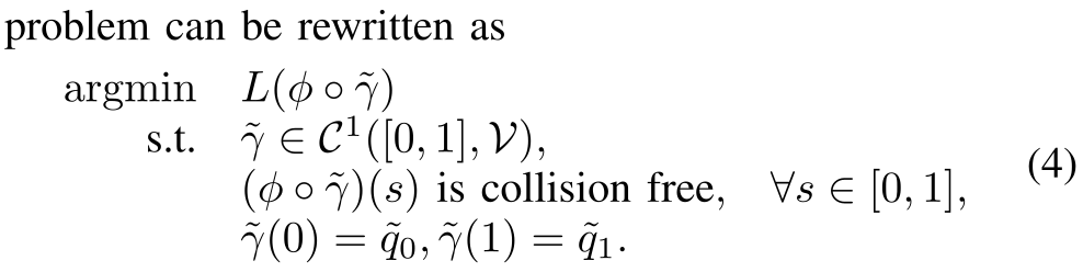
Equation1 separates reachable poses, continuous self-motion and discrete IK branches. The experiments hold a discrete branch fixed, and the continuous redundancy coordinates complete the local inverse. Equations3–4 express the same path problem in joint and minimal coordinates, provided the selected chart covers the required path. Direct reachability in Equation2 requires zero reconstruction residual everywhere feasible, motivating a less intrusive surrogate. Poses live on SE(3), so pose derivatives, Jacobian frames and local rotation coordinates must be consistent when implementing the formulas.
Original mathematical definitions, assumptions and experimental protocol
We use monogram notation [34, §3.1] to describe poses: is the pose of frame relative to (and expressed in) frame . When this pose is a function of a variable , we write . The forward kinematics are . An analytic IK function is a mapping

Original selectable mathematical display
Equation 1
| (1) |
Original mathematical definitions, assumptions and experimental protocol
where is a set of reachable end-effector poses, describes the continuous self-motions and enumerates the discrete self-motions (e.g. “elbow up” vs “elbow down”) [35]. In practice, we restrict ourselves to some and drop the discrete self-motion from the notation [10].

Original selectable mathematical display
Equation 2
| (2) |
Original mathematical definitions, assumptions and experimental protocol
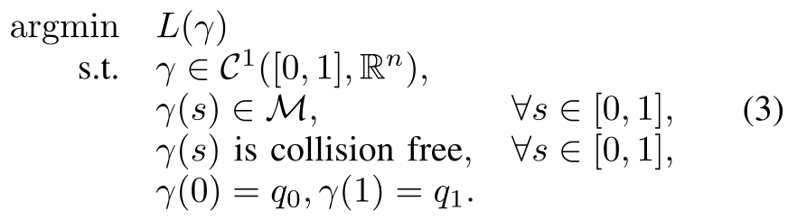
For a constraint manifold defined implicitly as , a minimum-cost path (with respect to a cost functional ) between can be found via
Original selectable mathematical display
Equation 3
| (3) |
Original mathematical definitions, assumptions and experimental protocol
Given a parameterization with , , and points such that and , this problem can be rewritten as
Original selectable mathematical display
Equation 4
| (4) |
Original mathematical definitions, assumptions and experimental protocol
For many constrained trajectory optimization problems, the equality constraint is the “hardest” constraint, so its elimination via an IK parameterization results in an easier-to-solve problem. We can interpret an optimization IK problem in the same way, by optimizing for a single point instead of a trajectory.
IV Methodology
The approach assumes access to analytic IK solutions with identifiable continuous/discrete self-motion and to forward-kinematics derivatives. It uses exact inverse differentiation where the augmented Jacobian is nonsingular, then numerical approximations where that reasoning fails. Approximate extension values and approximate derivatives are useful optimization guidance, not generally the derivative of the exact black-box projection procedure.
IV-A Applying the Inverse Function Theorem
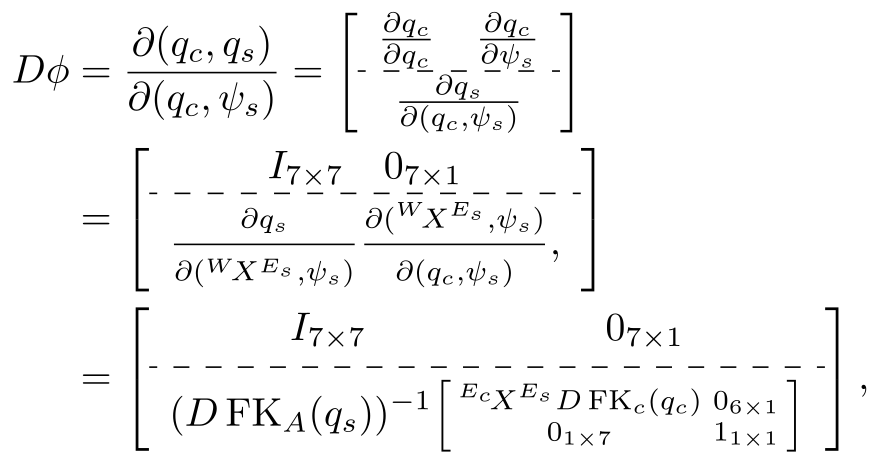
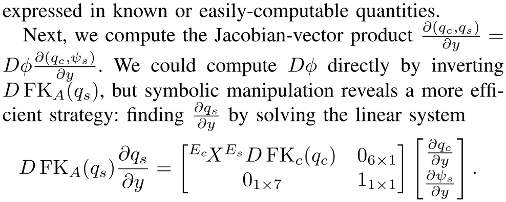
The preserved theorem gives a local inverse near a regular point. Stacking the ordinary FK Jacobian with derivatives of self-motion coordinates makes the augmented map locally square and invertible. Equation6 obtains Jacobian-vector products by solving against this augmented Jacobian rather than differentiating generated IK code or explicitly forming its inverse. The bimanual example retains the complete block-Jacobian derivation and final linear solve. Fixed branch identity gives consistent redundancy choices, while rank loss, representation singularities and branch changes invalidate a single smooth inverse; the construction is not a global convergence theorem.
Theorem 1 (Inverse Function Theorem).
If is continuously differentiable at a point and has a full-rank Jacobian, then there is an inverse function defined on a neighborhood of , and .
Original mathematical definitions, assumptions and experimental protocol
For a nonredundant manipulator, the EE pose uniquely identifies the joint angles up to the choice of discrete self-motion , so . For a redundant manipulator, we call the inverse of the analytic IK function the augmented forward kinematics (inspired by the language of Elias and Wen [17]). We write and restrict to a single discrete self-motion ; its Jacobian will have the block structure

Original selectable mathematical display
Equation 5
| (5) |
Original mathematical definitions, assumptions and experimental protocol
where maps the joint angles to their corresponding self-motion parameter. If joint angles are used to parameterize the self motion (as in IKFast [14]), the rows of are standard basis vectors. For a 7DoF arm using the shoulder-elbow-wrist parameterization, it is still simple to compute this Jacobian [17].
Original mathematical definitions, assumptions and experimental protocol
Now, we leverage to compute gradients of the analytic IK mapping. Suppose we have decision variables and partials for some other variable . We obtain , and want to compute . Due to the IFT, , so we find by solving the linear system

Original selectable mathematical display
Equation 6
| (6) |
Original mathematical definitions, assumptions and experimental protocol
This is analogous to how differential inverse kinematics (DiffIK) resolves kinematic redundancy locally, but our use of the augmented Jacobian ensures global consistency. For non-reachable configurations (and representational singularities [17]), loses rank, and the IFT breaks down. In this case, we fall back to an approximate solution (details deferred to Subsection IV-B).
Original mathematical definitions, assumptions and experimental protocol
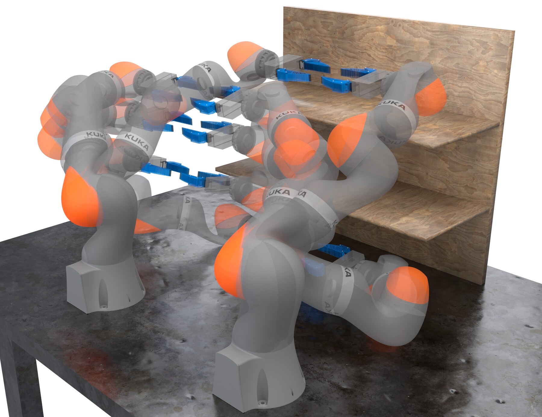
A worked example. We now discuss how to apply the IFT machinery to a parameterization for constrained bimanual motion planning [10]. Let be the joint angles of the “controlled” and “subordinate” arms, and their end-effector frames, and let be the subordinate arm’s continuous self-motion parameter. Let be the forward kinematics of the controlled arm and refer to the augmented forward kinematics of the subordinate arm. We compute the desired pose of the subordinate arm’s end-effector in terms of via , where is the fixed transform between the end-effectors. Then we compute , obtaining the full configuration . Thus, parameterizes the constraint manifold, and we wish to compute the derivatives

Original selectable mathematical display
Equation
Original mathematical definitions, assumptions and experimental protocol
First, the Jacobian of has the organized block structure
Original selectable mathematical display
Equation
Original mathematical definitions, assumptions and experimental protocol
Next, we compute the Jacobian-vector product . We could compute directly by inverting , but symbolic manipulation reveals a more efficient strategy: finding by solving the linear system
Original selectable mathematical display
Equation
IV-B Extending the Domain of IK
Equation7 defines an ideal least-squares extension, and Equation8 differentiates a smooth local optimum using its residual-weighted Hessian. This sensitivity formula needs a locally well-defined optimum and nonsingular local Hessian; it is not automatically valid at nonunique projections or branch transitions. The implementation instead uses efficient clipping, geometric subproblem approximations or bisection toward a nominal reachable target. The six gradient strategies below therefore approximate the extension and can disagree with the actual projection derivative.
Original mathematical definitions, assumptions and experimental protocol
To examine how to compute the gradients in these conditions, we interpret the various methods for extending the domain of as approximations of

Original selectable mathematical display
Equation 7
| (7) |
Original mathematical definitions, assumptions and experimental protocol
For reachable , . Otherwise, returns a configuration that achieves the closest end-effector pose in a least-squares sense.
Original mathematical definitions, assumptions and experimental protocol
We can compute via sensitivity analysis. Let be the optimum, the augmented Jacobian, the augmented task-space residual, and the Hessian slice corresponding to the th row of . Then

Original selectable mathematical display
Equation 8
| (8) |
Original mathematical definitions, assumptions and experimental protocol
Observe that if is reachable, the residual , so . Thus, if is full rank, we recover the IFT formulation. Also, this matrix inversion (and those in the following approximations) can be avoided with linear system solves, analogous to (6).
IV-B 1 Zero Gradients
Zero gradients avoid numerical explosions but discard useful information about how an infeasible target should move toward reachability. This reproduces a prior fallback and performs poorly for the counterexample-search task under direct reachability, though it remains a comparison baseline.

Original selectable mathematical display
Equation 9
| (9) |
IV-B 2 Pseudoinverse
The pseudoinverse keeps sensitivity in nonzero singular directions while removing null directions. It omits the residual-Hessian term of the exact local least-squares derivative. Singular-value thresholds and numerical conditioning still matter; a pseudoinverse does not make the original inverse-function theorem apply at a rank-deficient point.
Original mathematical definitions, assumptions and experimental protocol
If is singular, this should still preserve gradient flow in the non-singular directions while avoiding a numerical blowup.

Original selectable mathematical display
Equation 10
| (10) |
IV-B 3 Levenberg-Marquardt (LM)
Levenberg–Marquardt adds isotropic damping to the normal equations. The paper compares a constant value with damping activated by the smallest singular value. This stabilizes a surrogate inverse while biasing the derivative. All threshold formulas and conditions remain in the original mathematical context below.

Original selectable mathematical display
Equation 11
| (11) |
IV-B 4 Residual Damping
Residual damping increases regularization as the pose/self-motion mismatch grows. It uses information unavailable to zero or undamped pseudoinverse gradients, and gives strong downstream results in this study. Its weighting depends on how translation, rotation and redundancy residuals are represented and scaled.

Original selectable mathematical display
Equation 12
| (12) |
IV-B 5 Anisotropic Damping
Anisotropic damping uses the Jacobian’s singular directions and residual alignment to set direction-specific regularization. It is more structured than isotropic damping, but not uniformly faster: Table I’s direct-reachability Trajopt time 2.52 s exceeds several simpler alternatives. The original SVD definitions and damping expression remain intact.
Original mathematical definitions, assumptions and experimental protocol
A damping factor is introduced along each singular direction that scales with the magnitude of the residual in that direction. Let be the SVD, , . Then

Original selectable mathematical display
Equation 13
| (13) |
IV-B 6 Full Newton
The full-Newton variant adds residual-weighted kinematic Hessian slices plus damping. The implementation includes the six pose components; omitted self-motion Hessians vanish when self-motion is literally a joint angle, but need not vanish for other parameterizations. It is therefore not automatically the full exact sensitivity for every redundancy coordinate choice, and its added computation does not uniformly improve runtime.
Original mathematical definitions, assumptions and experimental protocol
Newton’s method is well-understood for least-squares problems [40, §10]. We only use the first components of the augmented kinematic Hessian, corresponding to the end-effector pose, as these can be obtained in closed-form [41]. When self-motion is parameterized by the angle of one or more joints, that Hessian component vanishes; otherwise we would require second-order autodiff.

Original selectable mathematical display
Equation 14
| (14) |
Original mathematical definitions, assumptions and experimental protocol
We emphasize that we do not compute the least-squares solution in practice, but instead rely on efficient approximations: clipping [10], geometric subproblem least-squares [20, 21], or even a simple bisection search to a canonical reachable target (used for our RB-Y1 experiment).
IV-C New Reachability Constraints
The reachability argument assumes that an unreachable target’s extended IK solution lies on the actual reachable boundary, where ordinary FK loses rank. Equation15 uses a finite, regularized log determinant and a tuned threshold to discourage that boundary; Equation16 provides its derivative. This practical surrogate depends on ε,τ, Jacobian scaling and the chosen extension. A finite regularized determinant bound is not an unconditional minimum-singular-value certificate: large other singular values can compensate for a small or zero one. Nor does the argument apply to an arbitrary approximate solver returning an interior point for an unreachable target. These are scope conditions, not evidence that the reported robot runs accepted infeasible targets.
Original mathematical definitions, assumptions and experimental protocol
The boundary of the reachable workspace is composed of critical values, i.e., a configuration in the preimage of the boundary must have low-rank Jacobian [23, §3.3]. projects onto the boundary of the reachable set, a property maintained by all three approximations used in our experiments. Thus, enforcing non-singularity of the kinematic Jacobian is sufficient for enforcing reachability. Let and (the ordinary kinematic Jacobian), then our boundary reachability constraint is

Original selectable mathematical display
Equation 15
| (15) |
Original mathematical definitions, assumptions and experimental protocol
for hyperparameters and , which must be chosen on a per-problem basis. We use this log-determinant formulation for its well-behaved gradients: the constraint gradient can be compiled from the following partial derivatives

Original selectable mathematical display
Equation 16
| (16) |
Original mathematical definitions, assumptions and experimental protocol
together with the chain rule and obtained from any of the methods in Subsection IV-B. Computing (16) requires the kinematic Hessian, a more expensive computation than direct reachability, which only needs the kinematic Jacobian. But in practice, boundary reachability outperforms direct reachability, thanks in part to its better optimization properties.
V Experiments
The experiments separate derivative correctness on reachable samples, downstream runtime with different reachability treatments, generic-solver grasp optimization, and hardware execution. Each addresses a different question. Agreement with autodiff inside a regular chart does not validate exact out-of-domain gradients, and a runtime benefit in one task need not carry over to another optimizer or derivative-vector size.
Accessible original table, all values and grouped headers
| Gradient Method | IrisNp2 | Trajopt | TOPPRA |
| Autodiff Baselines | |||
| Autodiff, Direct Reachability | 1.14 | 1.54 | 0.59 |
| Autodiff, Probing Reachability | 1.03 | 0.98 | 0.60 |
| Autodiff, Boundary Reachability | 1.08 | 1.24 | 0.58 |
| Proposed: IFT, Direct Reachability | |||
| IFT, Zero Gradients (9) | 4.11 | 1.35 | 0.75 |
| IFT, Pseudoinverse (10) | 4.12 | 1.31 | 0.81 |
| IFT, LM Constant (11) | 3.12 | 1.42 | 0.80 |
| IFT, LM SVT (11) | 2.22 | 1.49 | 0.80 |
| IFT, Residual Damping (12) | 1.58 | 1.76 | 0.81 |
| IFT, Anisotropic Damping (13) | 1.72 | 2.52 | 0.81 |
| IFT, Full Newton (14) | 1.71 | 1.43 | 0.82 |
| Proposed: IFT, Boundary Reachability | |||
| IFT, Zero Gradients (9) | 1.64 | 1.20 | 0.75 |
| IFT, Pseudoinverse (10) | 1.75 | 1.23 | 0.80 |
| IFT, LM Constant (11) | 2.51 | 1.31 | 0.80 |
| IFT, LM SVT (11) | 1.29 | 1.21 | 0.80 |
| IFT, Residual Damping (12) | 1.15 | 1.24 | 0.81 |
| IFT, Anisotropic Damping (13) | 1.15 | 1.23 | 0.81 |
| IFT, Full Newton (14) | 1.17 | 1.20 | 0.82 |
V-A Comparison with Forward-Mode Autodiff
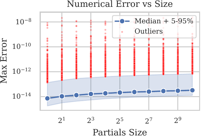
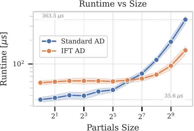
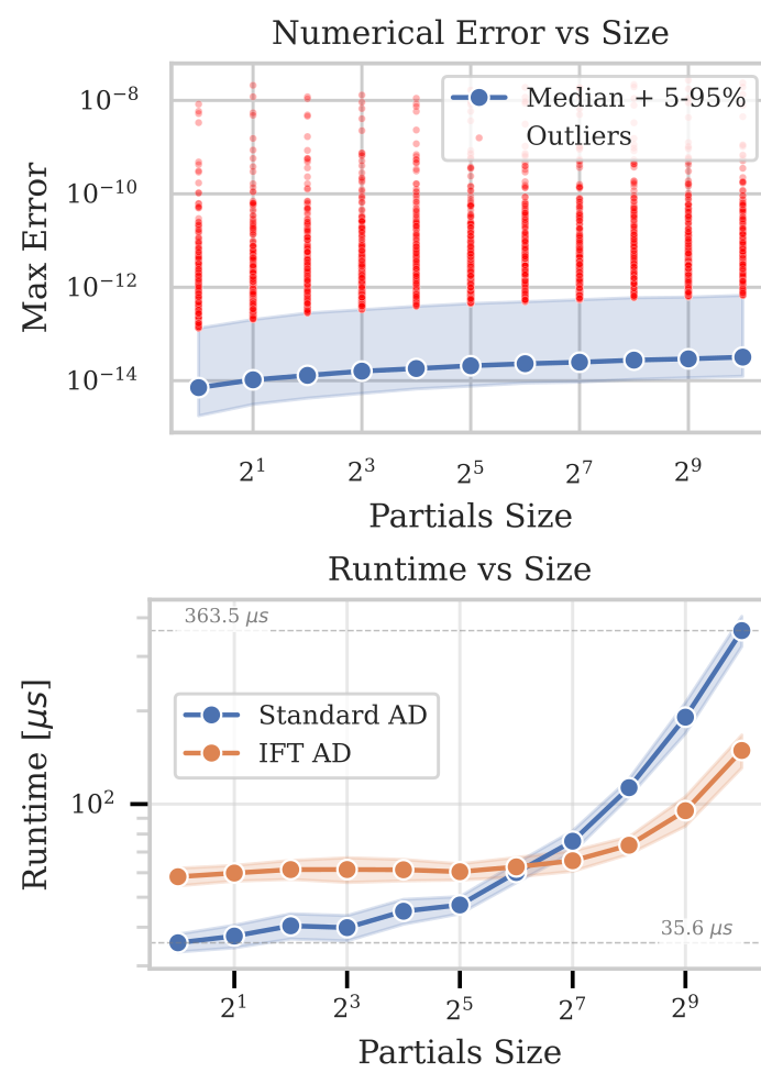
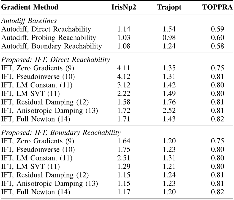
On 10,000 sampled reachable configurations, median derivative error is below 10⁻¹³ and the 95th percentile below 10⁻¹²; Figure2 also retains the higher-error outliers. The trial partials are random synthetic derivative directions, not physical trajectories. Standard forward autodiff is faster through partial size 2⁶; IFT gains for larger vectors by amortizing Jacobian construction, while both curves still have solve costs. Downstream Table I averages IrisNp2 over 17 seeds,Trajopt over 10 RRT-initialized solves,and timing over three trajectory families. Boundary/residual IFT gives IrisNp2 1.15 s versus 1.08 s for autodiff with the same constraint, but TOPPRA 0.81 s versus 0.58 s is roughly 40% slower. Direct-reachability IFT can be much slower, and boundary is not best for every metric. These results support compatibility and selected near-baseline timings, not a blanket speedup.
Original mathematical definitions, assumptions and experimental protocol
We evaluate the derivatives for the bimanual parameterization in isolation with low-level calculations, and we examine high-level performance on downstream tasks. Let denote a point in the parameterized space and a point in C-space.
Original mathematical definitions, assumptions and experimental protocol
First, we examine speed and accuracy of the derivative calculations themselves. We sample reachable configurations (with rejection sampling). For each configuration , for a range of decision variable sizes , we sample vectors of partial derivatives . (Note that in these experiments, the partials do not correspond to any physical quantities; we are purely evaluating the speed and accuracy at the autodiff level.) For each , we compute via forward-mode autodiff and our IFT technique. The median error for each partial size is less than , and the 95th percentile is less than . Autodiff is fastest up to partial size , but for larger partial sizes, IFT is faster, due to constant cost of building the augmented Jacobian . Full numerical results are shown in Fig. 2.
V-B Using Generic IK Solvers
EAIK and IKFast demonstrate using generated solvers without rewriting them for autodiff. They still require branch/redundancy management and a usable extension outside the reachable domain. The selected examples establish practical applicability to these mechanisms and tasks, while cuspidal robots and unsorted polynomial IK branches remain open cases.
V-B 1 Using a Solution Generated by EAIK
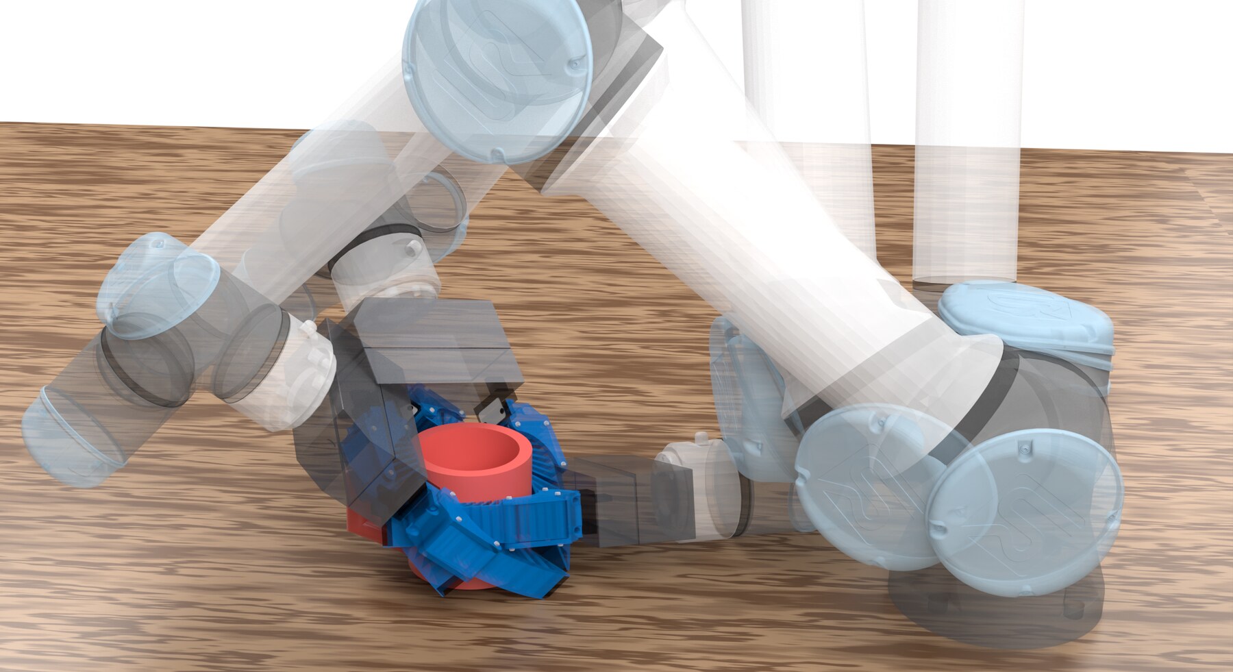
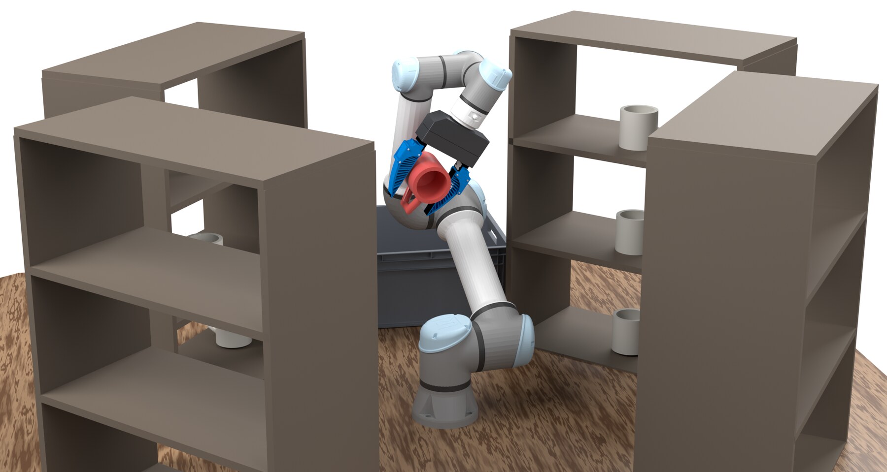
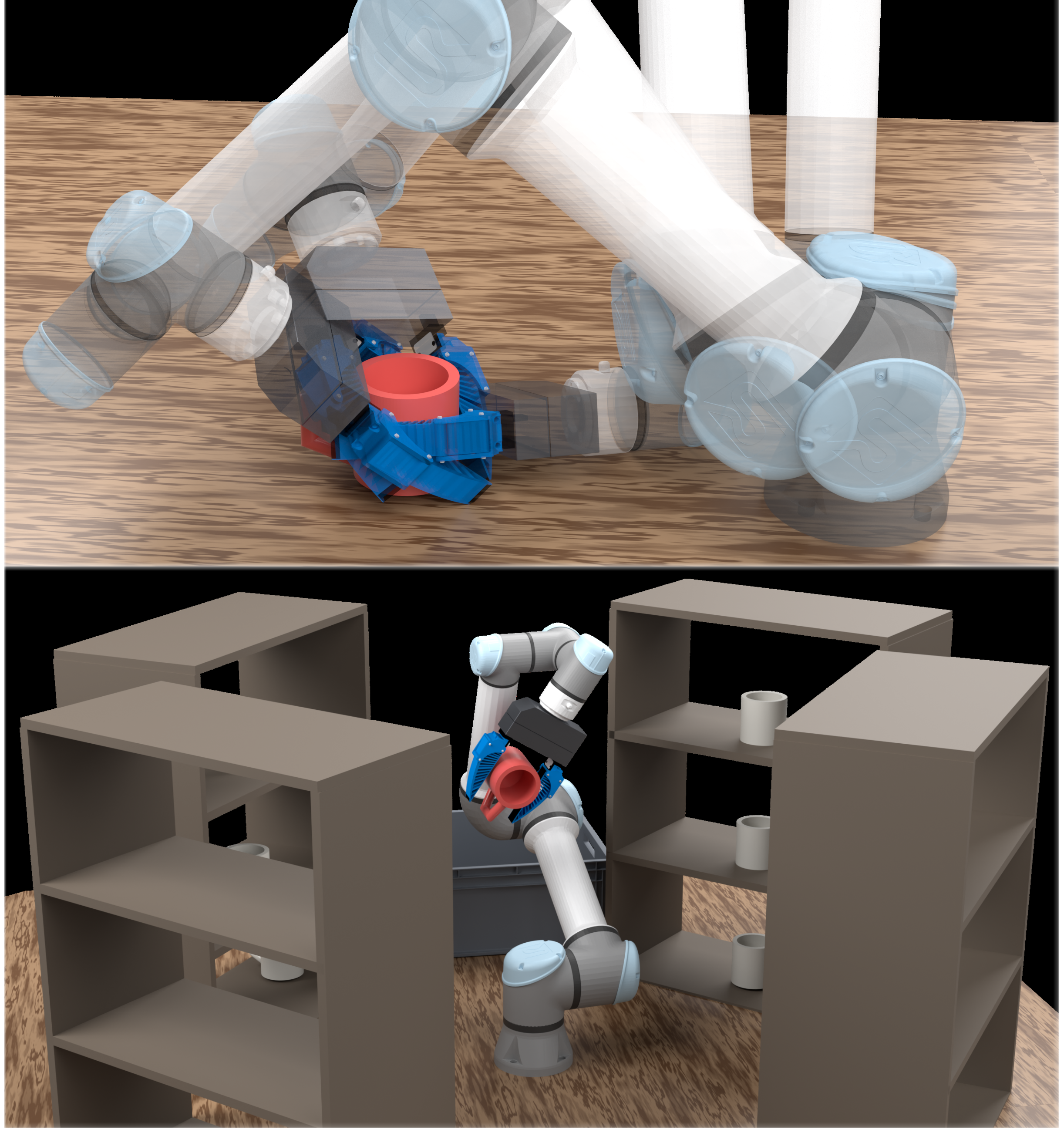
A UR5e selects mug grasps with joint-centering cost, ±π joint limits, collision avoidance and a constrained gripper centerline. One hundred feasible sampled problem instances each get ten shared initializations; those starts also choose the IK branch. Table II reports single-start success 46.5% baseline versus 61.4/63.2% direct/boundary IFT, and three-start success 86% versus 93/90%. Repeated starts on the same instance are not independent new scenes. IFT mean runtimes 0.719/0.776 s are about 2.0/2.17× baseline 0.357 s, although medians are similar. Cost comparisons in parentheses use mutual successes: direct IFT mean 12.57 is slightly lower than baseline 12.81, so higher cost is not universal. Approximate gradients may complicate line-search convergence; the proposed trust-region alternative is not tested here.
Original selectable mathematical display
Equations 17a–17d
| (17a) | ||||
| (17b) | ||||
| (17c) | ||||
| (17d) | ||||
Original mathematical definitions, assumptions and experimental protocol
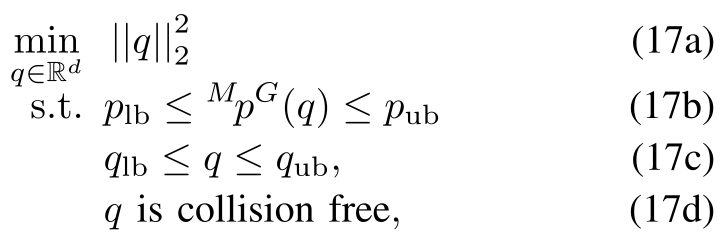
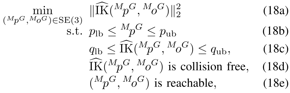
where is the body frame of the manipuland and denotes the position of the gripper in the manipuland frame. We set the joint limits to . (17b) enforces that a point between the fingers lie along the centerline of the mug, effectively a nonlinear equality constraint. This can be rewritten as an optimization problem in minimal coordinates space via the IK change-of-variables:
Original selectable mathematical display
Equations 18a–18e
| (18a) | ||||
| (18b) | ||||
| (18c) | ||||
| (18d) | ||||
| (18e) | ||||
Original mathematical definitions, assumptions and experimental protocol
where we have separated the pose of the gripper into the position and orientation for notational convenience.
Original mathematical definitions, assumptions and experimental protocol
We compare the ordinary configuration-space formulation (17) with the end-effector parameterized formulation (18), using both the direct reachability and boundary reachability constraints, with SNOPT [19] as the optimizer. For direct reachability, we did not square the norm as in (2); this decision empirically led to better performance on this problem instance. We use IFT residual damping to compute .

Accessible original table, all values and grouped headers
| Formulation | Success Rate (Multistart) | Mean Cost | Median Cost | Mean Runtime | Median Runtime | |
| 1 init | 3 init | |||||
| (17), C-Space Baseline | 46.5% | 86% | 12.68 (12.81) | 10.94 (11.11) | 0.357 (0.365) | 0.105 (0.096) |
| (18), IFT, Direct | 61.4% | 93% | 13.30 (12.57) | 12.65 (11.95) | 0.719 (0.720) | 0.100 (0.083) |
| (18), IFT, Boundary | 63.2% | 90% | 13.53 (13.03) | 12.83 (12.66) | 0.776 (0.825) | 0.110 (0.095) |
V-B 2 Using a Solution Generated by IKFast
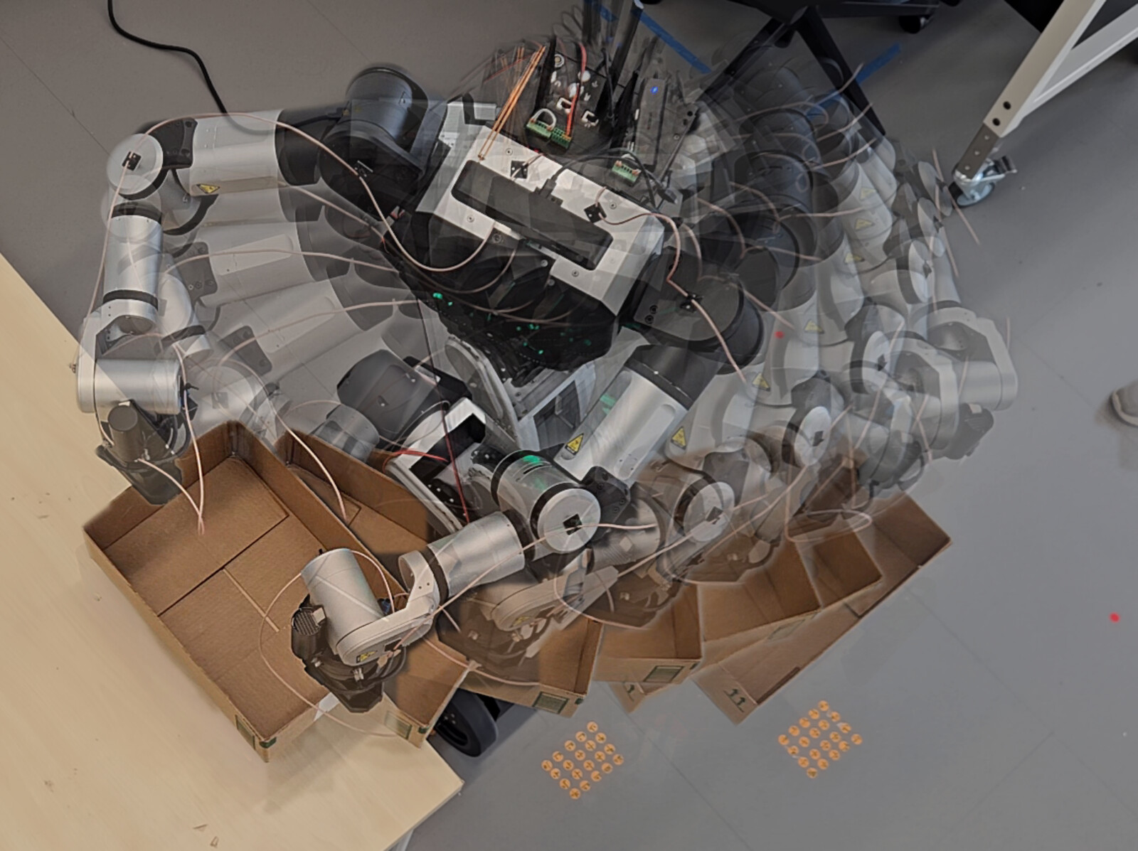
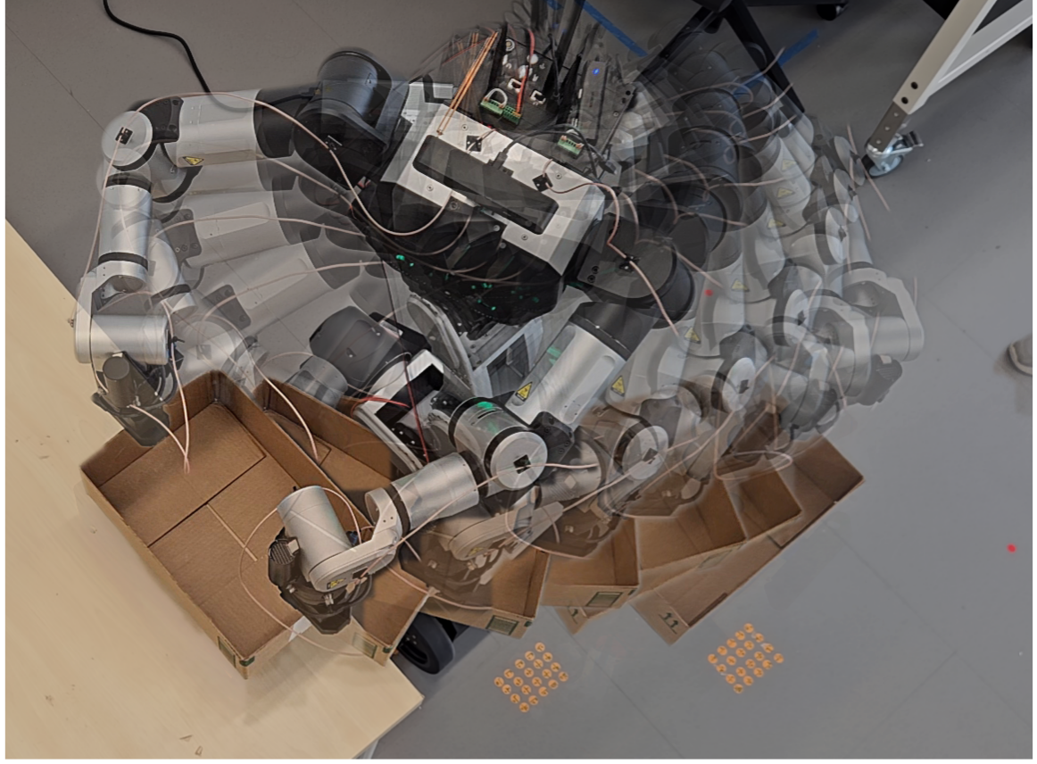
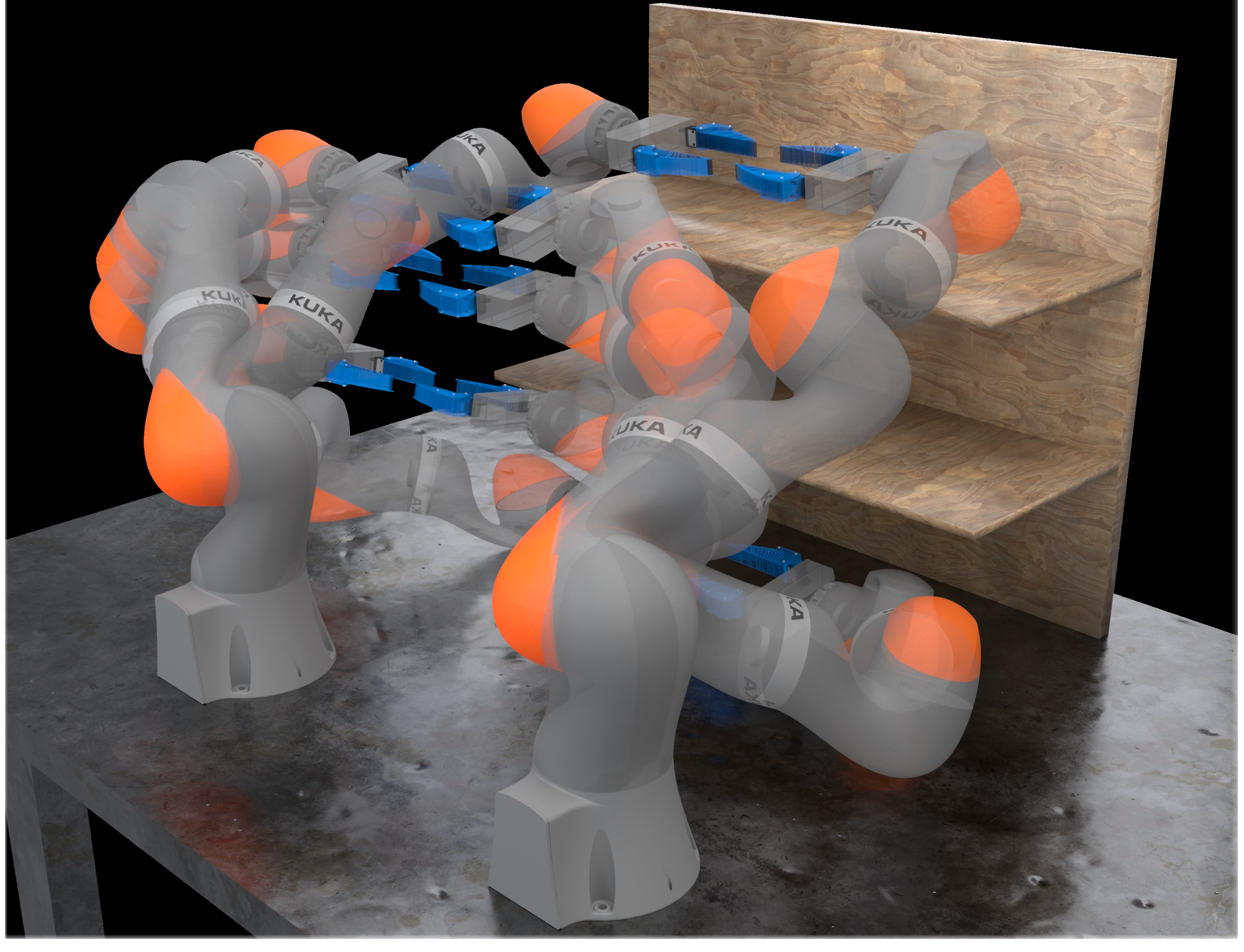
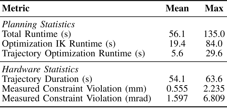
IKFast parameterizes both RB-Y1 arms, with base pose fixed, torso variables and arm self-motion coordinates. Twenty floor positions form a 4×5 grid at 3 cm spacing for the same box/table setup. Six sequential motion phases combine grasp selection, straight-line checks/BiRRT,shortcutting,Trajopt and TOPPRA, with static center-of-mass support constraints. The extension uses bisection toward a nominal reachable target plus residual damping. Mean planning time is 56.1 s (max 135),distinct from 54.1 s execution. Measured relative-constraint violation averages 0.555 mm/1.597 mrad,with maxima 2.235 mm/6.809 mrad; floating-point exactness describes the planned kinematics, not actual hardware tracking. The official project reports 20/20 trials and links the recording. This is limited same-object/grid evidence, not a general contact/dynamics or safety guarantee.
Original mathematical definitions, assumptions and experimental protocol
In our second experiment, we use IKFast to derive a solution for the arms of a Rainbow RB-Y1 robot. We then construct a parameterization that enables it to move objects with both hands, while maintaining a constant relative end-effector transform. In particular, given analytic IK solutions and for the left and right arms respectively, our parameterization is

Original selectable mathematical display
Equation
Original mathematical definitions, assumptions and experimental protocol
where and are the joint angles of the RB-Y1’s base and torso respectively, are the self-motion parameters of the left and right arms, and is the world frame. is kept fixed in this experiment.
Original mathematical definitions, assumptions and experimental protocol
The robot’s task is to pick up a box and place it on a nearby table from a set of starting positions arranged in a grid (points spaced 3cm apart) on the floor in front of the robot’s base, for a total of 20 trials. Each pick-and-place trajectory is composed of six parts, planned sequentially:
Accessible original table, all values and grouped headers
| Metric | Mean | Max |
| Planning Statistics | ||
| Total Runtime (s) | 56.1 | 135.0 |
| Optimization IK Runtime (s) | 19.4 | 84.0 |
| Trajectory Optimization Runtime (s) | 5.6 | 29.6 |
| Hardware Statistics | ||
| Trajectory Duration (s) | 54.1 | 63.6 |
| Measured Constraint Violation (mm) | 0.555 | 2.235 |
| Measured Constraint Violation (mrad) | 1.597 | 6.809 |
VI Discussion
The useful result is an implementation-independent local derivative interface for suitably continuous IK charts, supplemented by effective approximate gradients and problem-tuned reachability treatment. The paper explicitly leaves branch tracking for unsorted solutions and cuspidal manipulators open. Fixed-chart planning can reason beyond purely local differential IK, but still uses nonlinear optimization and initial guesses; it does not guarantee global optimality or cover every component of the constraint set.
Acknowledgement
The source credits Aditya Agarwal and Lucy Cai for RB-Y1 communication infrastructure and Shrutheesh Iyer for kinematics insights. Equal-contribution marks for Thomas Cohn and Seiji Shaw and the paper’s institutional/support information remain associated with the original source.
Original diagrams and demonstration recordings
Original project images and the boundary-reachability animation are preserved locally with the source movie and a derived preview poster. The original overview and RB-Y1 hardware recording remain linked on YouTube, including the project’s twenty-trial montage. The animation illustrates the constraint value; it is not an additional hardware success experiment. These recordings do not add independent trials to the paper’s twenty runs.