At a glance
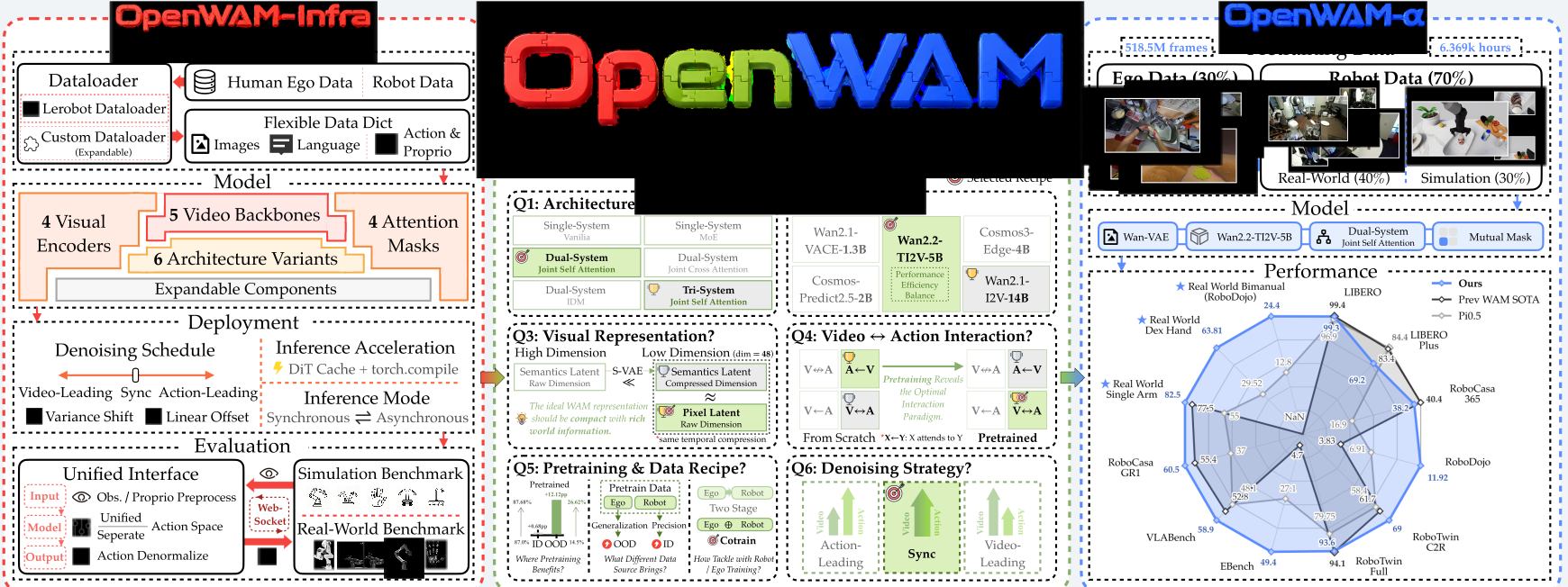
OpenWAM makes world–action modeling a configurable research stack, studies the effect of its components, and scales the resulting recipe into OpenWAM-α. The model jointly learns future video and executable actions from 518.5 million frames, representing 6,369 hours of human and robot data.
Its main contribution is a reproducible way to compare coupled design choices. The experiments favor capable video priors, compact visual latents, dedicated action capacity, and joint training. These are empirical results under the tested settings, not universal optimality claims. This edition retains all 43 pages’ figures, tables, equations, references, and appendix protocols from arXiv v1, dated 7 September 2026.
1. Introduction
Video generation supplies knowledge of how scenes evolve; robot demonstrations connect that knowledge to controllable actions. Yet a system’s backbone, representation, fusion architecture, data, and inference procedure often change together, making improvements difficult to attribute.
OpenWAM separates three questions: which upstream knowledge to inherit, how world and action prediction should interact, and how embodied pretraining changes generalization. Infra supplies the controlled implementation, Study accumulates an experimental recipe, and α instantiates that recipe at scale.
3. OpenWAM-Infra
One stack covers data ingestion, model construction, training, serving, and evaluation. Changing a component should not require rewriting the trainer or benchmark client. Checkpoints include the information required to rebuild both the model and its action normalization.
3.1 Composable model
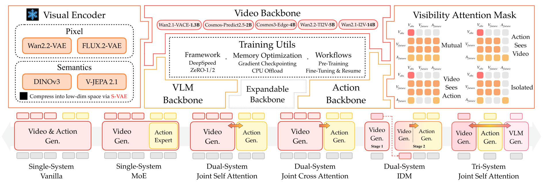
A model is the composition C(E, S, M): a frozen visual encoder E, one or more stream backbones S, and a visibility mask M. The encoder maps observations to latents; world, action, and optional understanding streams process them; the mask controls which tokens can exchange information.
Every backbone exposes preparation, per-layer execution, and finalization. Attention can be replaced at a layer boundary without changing the backbone internals. The composition rule itself has no learned parameters.
Visual encoders, backbones, and attention masks
Reconstruction encoders include Wan2.2-VAE and FLUX.2-VAE; representation encoders include DINOv3 and V-JEPA 2.1, optionally compressed with S-VAE [81] [73] [63] [100]. Five video backbones are supported, from Wan-VACE 1.3B to Wan-I2V 14B, including Cosmos3-Edge-4B. Only four enter the controlled backbone comparison.
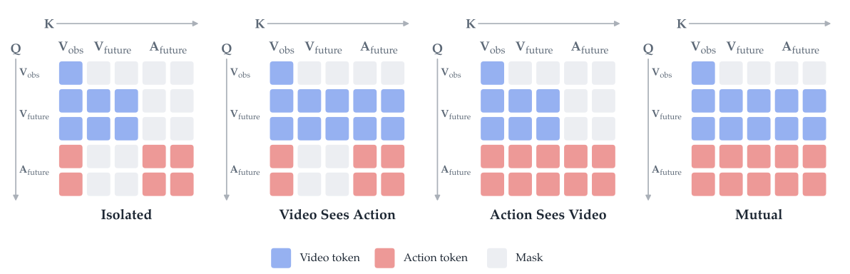
Equation 1 partitions visibility between video and action. The clean first video frame attends only to itself; future video tokens can communicate, and action tokens attend bidirectionally within their stream. Cross-stream blocks create isolated, video-sees-action, action-sees-video, or mutual interaction.
Equation

Architecture families
Single-system vanilla shares attention and feed-forward weights across video and action tokens. Its mixture-of-experts variant hard-routes action tokens through a separate feed-forward expert.
Dual systems use a dedicated action transformer. Joint self-attention merges the streams at bridge layers; cross-attention lets actions query video features, optionally stopping action-loss gradients into the video stream. The inverse-dynamics variant trains with teacher-forced video and generates video before actions at inference.
The tri-system variant adds a trainable understanding stream fed by a frozen vision–language model. This stream is a read-only tail: the other streams can attend to it, while it attends only to itself. Six variants become seven experimental rows when cross-attention is tested with and without detached gradients.
3.2 Training runtime
Each sample contains language, a video window, an action chunk, optional proprioception, and a dimension-validity mask. Time zero is noise and time one is clean data. Independent video and action noise levels train both velocity predictions through the flow-matching loss in Equation 2; clean conditioning frames are excluded from video loss.
Independent noise sampling covers the joint timestep plane and supports different inference schedules. It does not prove that all model-generated intermediate states have the same distribution as training examples.
The runtime supports mixed precision, gradient checkpointing, offload, and distributed optimization. Fine-tuning rebuilds a checkpoint’s modules; exact resume restores optimizer, scheduler, and data position and rejects changed normalization. Serving also rejects missing normalization statistics.
Equation

3.3 Deployment runtime
Serving mode and denoising schedule are separate choices. Synchronous serving waits for a fresh action chunk when the buffer empties. Asynchronous serving begins prefetch while d actions remain, skips the delayed prefix of the new prediction, executes the next n actions, and discards any unused tail.
The default lead threshold is n/2, with d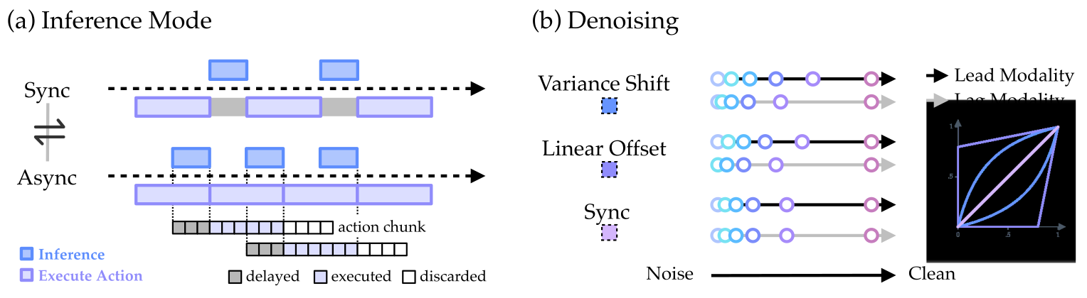
Denoising schedules
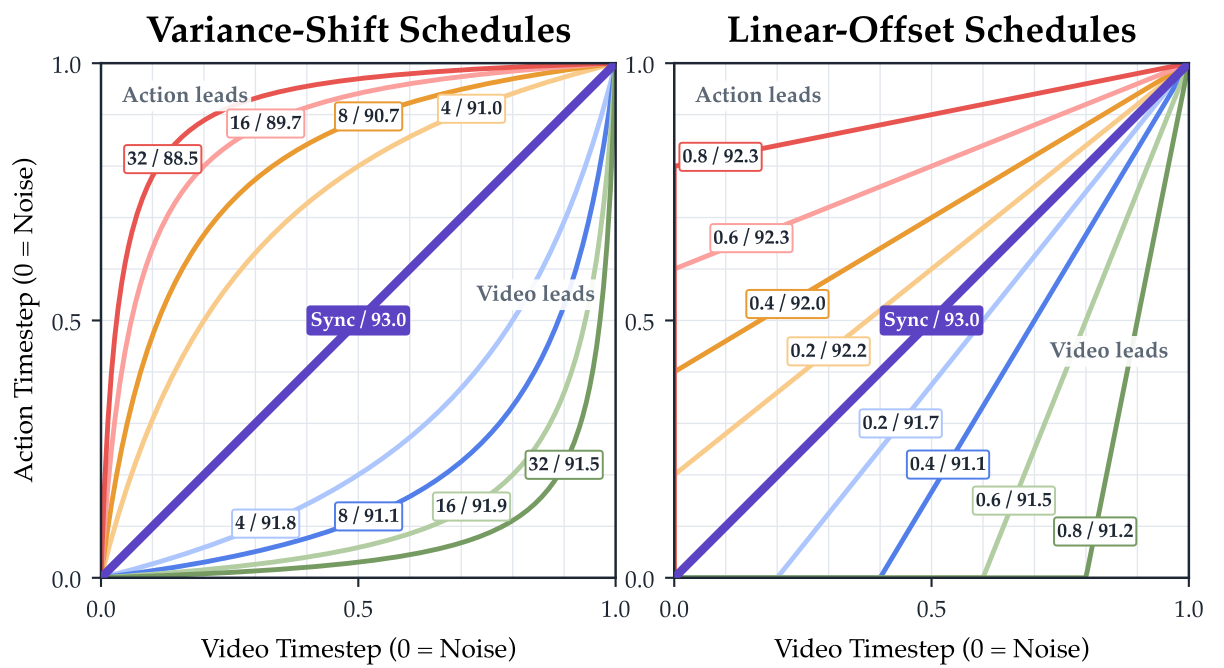
A schedule traces video and action timesteps from noise to clean data. Synchronized denoising follows the diagonal; variance shift accelerates a leading stream, while linear offset delays the other. Equation 3 preserves both functions. Choosing shift one and offset zero recovers the diagonal.
Each stream advances by its own Euler increment, and checkpointed timestep warps are reused at inference. These choices concern the prediction process within a chunk, independently of whether the robot server prefetches chunks.
Equation

Inference acceleration
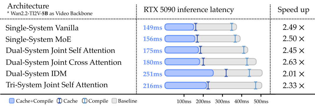
Four optimizations cache prompt embeddings, skip video decoding during control, compile fixed-shape denoising under CUDA graphs, and reuse similar velocity predictions for a bounded number of steps. Compilation adds first-request warmup.
Figure 4 reports 149–251 ms across architectures on an RTX 5090, including 175 ms for dual joint self-attention. Reported speedups of 2.01–2.63× compare compilation and velocity caching with a baseline that already caches prompts and skips video decoding. They are chunk-inference measurements, not continuous action frequencies.
3.4 Evaluation protocol
A benchmark sends images, language, and optional state over a persistent WebSocket connection and receives actions in native physical units. The server crops, resizes, normalizes, and composes up to three views, with a required head view and black-filled missing wrist views. Episode boundaries reset action buffers.
Adapters cover LIBERO, LIBERO-Plus, VLABench, RoboTwin2.0, RoboDojo, RoboCasa365, RoboCasa-GR1, and EBench. Keeping preprocessing and normalization with the checkpoint prevents silent coordinate changes between training and deployment.
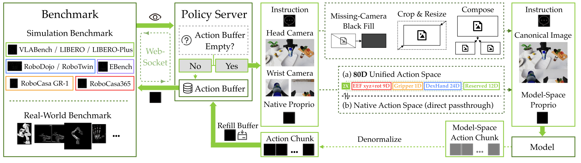
Action-space definition
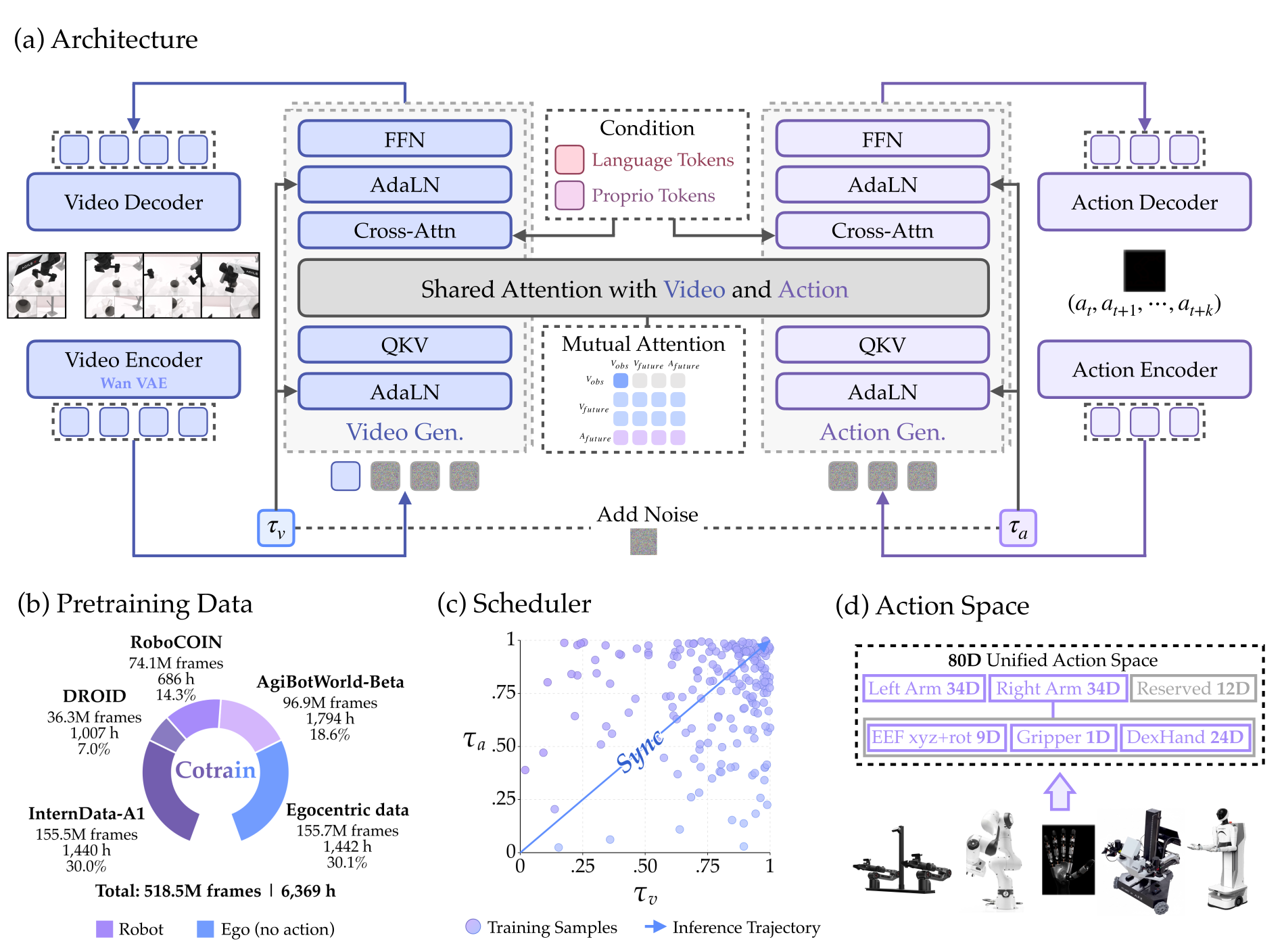
Single-benchmark models may retain native actions, such as 14-dimensional RoboTwin joints, 20-dimensional bimanual end-effector poses, or 10-dimensional LIBERO actions. Cross-embodiment α uses a shared 80-dimensional layout.
Each of two 34-dimensional arm blocks contains position, six-dimensional rotation, gripper state, and 24 hand coordinates; 12 additional slots are reserved for embodiment-specific channels. Equation 4 normalizes and scatters native coordinates into fixed slots, then gathers and denormalizes predictions. A validity mask removes unused coordinates from action-loss gradients.
Equation

4. OpenWAM-Study
The study sequentially holds the accumulated defaults fixed while varying one design axis. This is a controlled recipe-building exercise, not an exhaustive factorial comparison of every combination.
RoboTwin2.0-Full uses 2,500 clean and 25,000 randomized demonstrations across 50 tasks. Clean2Random instead fine-tunes only on clean demonstrations and evaluates both clean and randomized conditions. Its randomized success measures transfer after fine-tuning, not zero-shot deployment of the pretrained model.
4.1 Inheriting upstream world knowledge
The first question separates a video generator’s learned prior from the latent representation in which prediction occurs. A useful encoder must retain action-relevant information while keeping temporal and channel dimensions manageable.
4.1.1 Generative world priors
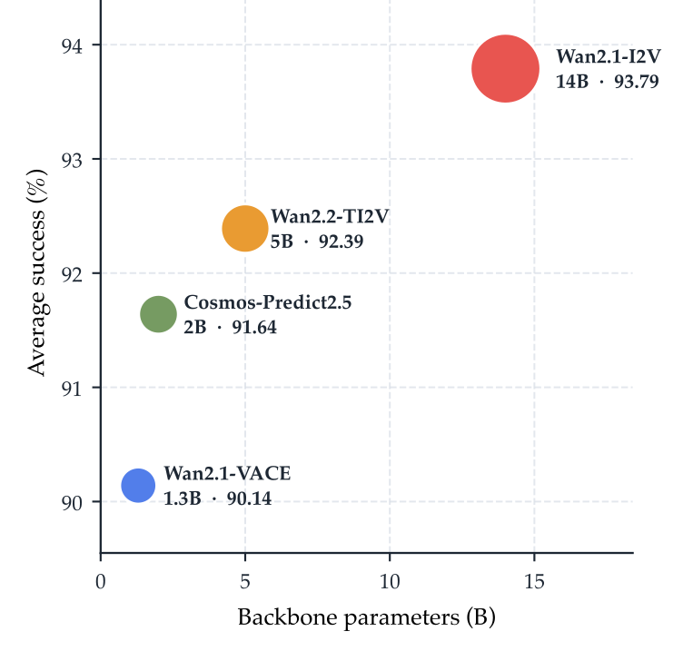
With otherwise matched settings, average success increases from 90.14% with Wan-VACE 1.3B to 91.64% with Cosmos-Predict2.5-2B, 92.39% with Wan2.2-TI2V-5B, and 93.79% with Wan2.1-I2V-14B. The 5B model becomes the practical default.
The backbones differ in pretraining data, architecture, and objective as well as size. Figure 6 therefore supports choosing a stronger available prior; it does not isolate a parameter-count scaling law.
4.1.2 Visual representation priors
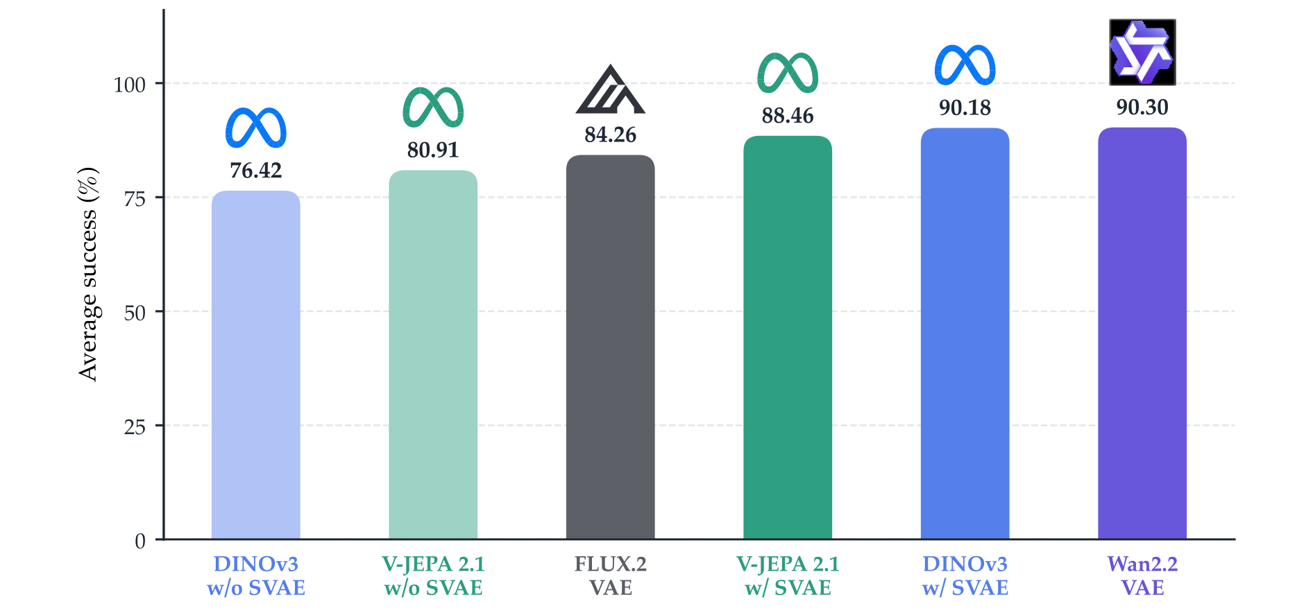
To isolate encoders, this experiment randomly initializes the video transformer instead of inheriting pretrained transformer weights. Non-Wan encoders average four consecutive frames for temporal compression; S-VAE reduces DINOv3’s 768 or V-JEPA’s 1,024 channels to 48.
Figure 7 reports 76.42% and 80.91% for uncompressed DINOv3 and V-JEPA, 84.26% for FLUX, 88.46% for compressed V-JEPA and 90.18% for compressed DINOv3, and 90.30% for Wan-VAE. Compact semantic representations nearly match the reconstruction encoder. Native learned temporal compression versus simple averaging remains a confound.
4.2 World–action interaction
The second question concerns dedicated action capacity and information exchange. The experiments distinguish architectural separation, attention visibility during training, and denoising order during inference.
4.2.1 Architectural capacity
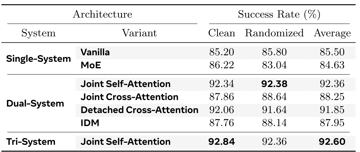
Table 1 reports 85.50% for single vanilla, 84.63% for single mixture-of-experts, 92.36% for dual joint self-attention, 88.25% for joint cross-attention, 91.85% for detached cross-attention, 87.95% for inverse dynamics, and 92.60% for the tri-system model.
Dual self-attention offers a strong balance of simplicity and accuracy. More parameters do not improve every variant: the single-system expert model is below vanilla, and the tri-system gain over dual is only 0.24 percentage points without uncertainty estimates.
4.2.2 Training-time information flow
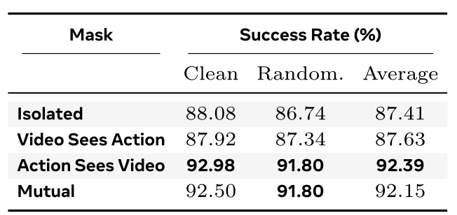
Action-sees-video reaches 92.39%, mutual visibility 92.15%, isolated streams 87.41%, and video-sees-action 87.63%. The large separation follows whether actions can access world features, supporting that connection within this configuration.
Here “from scratch” means without embodied pretraining; the system still inherits the video generator’s prior. It is distinct from the randomly initialized transformer used to isolate visual encoders.
4.2.3 Inference-time information flow
Figure 9 compares synchronization with variance-shift and linear-offset schedules on the same trained model. Synchronized joint denoising reaches 93.0%, above the tested action-leading and video-leading alternatives.
This supports joint refinement for the evaluated setup, and helps explain the weak two-stage inverse-dynamics baseline. It does not establish that every planning-based policy or every unequal schedule is inferior.
4.3 Consolidating knowledge across domains
The third question asks how embodied data changes the inherited prior and preferred world–action interaction. Broad human video offers scene coverage but lacks robot actions; demonstrations provide embodiment-specific control supervision.
4.3.1 Setup and evaluation
All runs hold architecture, backbone, fine-tuning, and inference fixed. A 600-hour pretraining budget compares robot-only RoboCOIN with a 350-hour EgoDex plus 250-hour robot mixture, trained sequentially or jointly. The budget matches total hours, not robot-action exposure.
Clean2Random separates clean-condition performance from randomized transfer. Full-data evaluation additionally checks behavior when downstream fine-tuning already includes both environments.
4.3.2 Pretraining and generalization
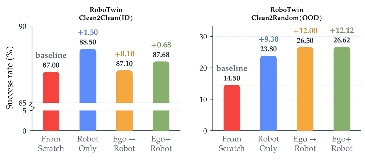
Without embodied pretraining, clean/randomized success is 87.0%/14.5%. Robot-only pretraining gives 88.5%/23.8%; sequential human then robot training gives 87.1%/26.5%; joint training gives 87.68%/26.62%.
The main gain is randomized transfer. Robot supervision improves clean execution more, while human-video coverage helps transfer. Joint and sequential mixtures differ by only 0.12 points on randomized conditions; absent uncertainty, joint training’s simpler workflow is a stronger justification than a claimed decisive accuracy gain.
4.3.3 Pretraining changes preferred information flow
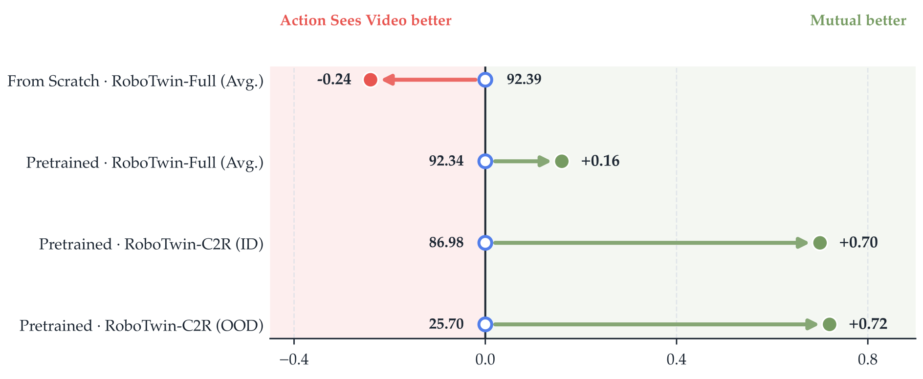
Before embodied pretraining, mutual attention is 0.24 points below action-sees-video. After pretraining, its gains are 0.16 points on RoboTwin-Full and 0.70/0.72 points on clean/randomized Clean2Random.
The recipe therefore changes to mutual visibility. Interpreting this as more useful action-conditioned world prediction is plausible, but the small performance differences do not directly identify the internal mechanism.
4.4 Resulting recipe
Table 3 retains the accumulated recipe: Wan2.2-TI2V-5B with compact latents, dual joint self-attention, synchronized denoising, and one-stage human-plus-robot training with mutual visibility. Each choice is conditional on the preceding defaults and evaluation protocol.

5. OpenWAM-α
OpenWAM-α combines the selected components in a model trained across heterogeneous data and embodiments. Figure 12 preserves the architecture, data mixture, timestep plane, and unified control layout. The original project overview video is retained below.
5.1.1 Architecture
A 5B video transformer and approximately 1B action transformer communicate at all 30 paired layers through shared attention with 24 heads of 128 dimensions. Their residual widths are 3,072 and 1,024. Video uses three-dimensional rotary positions; actions use one-dimensional positions.
A frozen Wan-VAE retains the clean first frame and compresses each subsequent group of four; patches are 1×2×2. Frozen umT5 supplies language context, with an additional projected proprioceptive token. Separate noise-time conditioning and output heads predict video and action velocities.
5.1.2 Training
Video, action, and proprioception projections are trained jointly; language and visual encoders stay frozen. Video and action loss weights are both one, with bell-shaped timestep weighting. Independent warped noise sampling emphasizes high-noise inputs.
The flow shift is five for both streams. Human videos without actions or proprioception contribute only video loss through masking; their visible hand motions are not robot-action annotations.
5.1.3 Deployment
Inference uses ten synchronized Euler steps with the same flow warp and repeatedly pins the clean conditioning frame. The accelerated model takes about 170 ms per action chunk on an RTX 5090 after warmup.
Every reported simulation and real-robot benchmark uses synchronous serving: execution pauses for inference between chunks. The number is not evidence of uninterrupted real-time control under asynchronous deployment.
5.2 Multi-domain pretraining data
Curation reduces 1,333.9 million raw frames, or 14,348 hours, to 518.5 million frames and 6,369 hours. Table 4 retains every source’s raw and retained counts, frame rate, embodiment coverage, and sampling share.
The retained pool includes 1,442 hours of new egocentric video, 1,794 AgiBotWorld-Beta, 686 RoboCOIN, 1,007 DROID, and 1,440 synthetic InternData-A1 hours. It spans 21 robot embodiments plus human video [13] [87] [40] [78].

5.2.1 Mixture and sampling
The human source begins with 71,600 first-person recordings spanning 3,006 tasks, each approximately 0.25–6 minutes long. Whole episodes are subsampled with fixed seeds and source budgets; real-robot budgets are redistributed across contributing subdatasets.
The approximate 30% human, 40% real-robot, and 30% synthetic mixture is a frame/sample ratio, not an hour ratio: sources have different frame rates. Proportional sampling draws each retained example once per epoch.
5.2.2 Data curation
Visual filtering removes unreadable, frozen, blurred, badly exposed, or abruptly discontinuous video. Human recordings also require visible manipulating hands and valid language annotations.
Robot episodes fail integrity checks when commanded and recorded motion disagree excessively or video–signal misalignment exceeds 2%. Leading and trailing idle spans are trimmed using state thresholds and motion below 2 cm/s and 5°/s; pauses within a trajectory are preserved. Median-absolute-deviation rules remove spikes, and visual checks catch sensor motion over frozen views.
Episodes are dropped if more than 70% of frames are removed or at least 90% are frozen. These rules and source budgets jointly determine what actually reaches pretraining.
5.3 Simulation evaluation
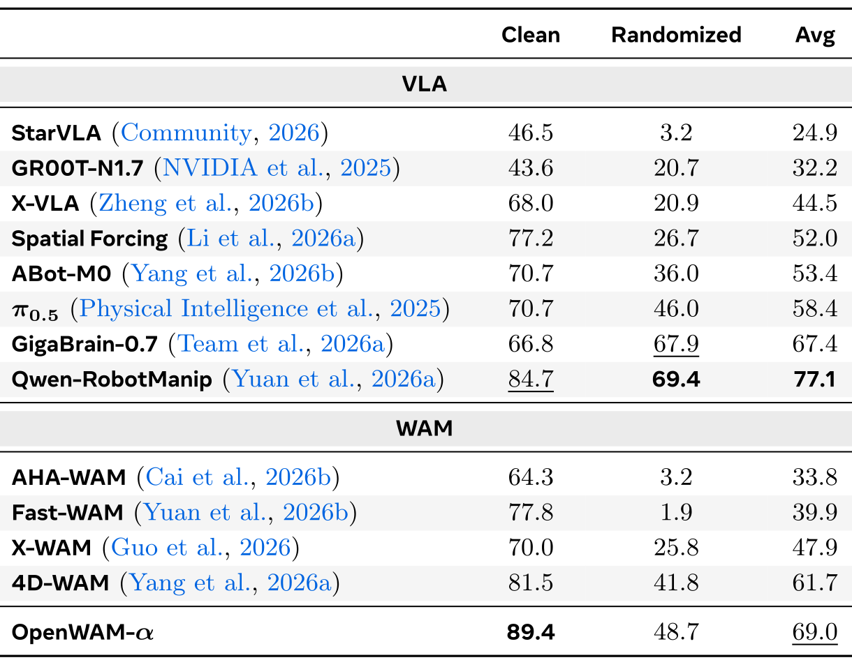
The pretrained checkpoint is separately fine-tuned for eight simulation benchmarks spanning single-arm, bimanual, mobile, and dexterous manipulation. RoboTwin-Full and Clean2Random are distinct evaluations of the same benchmark family.
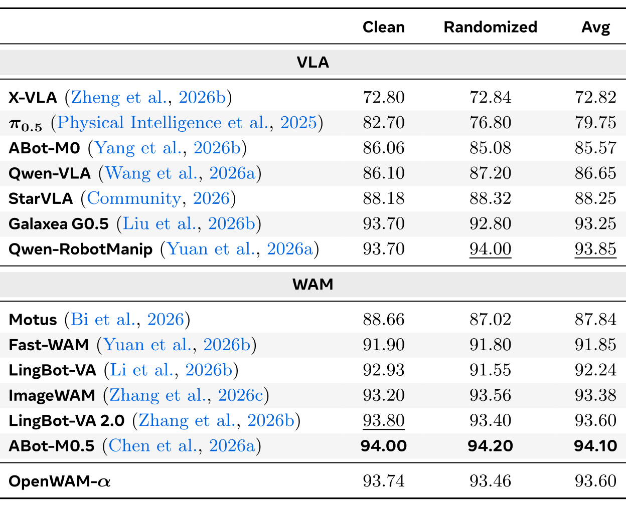
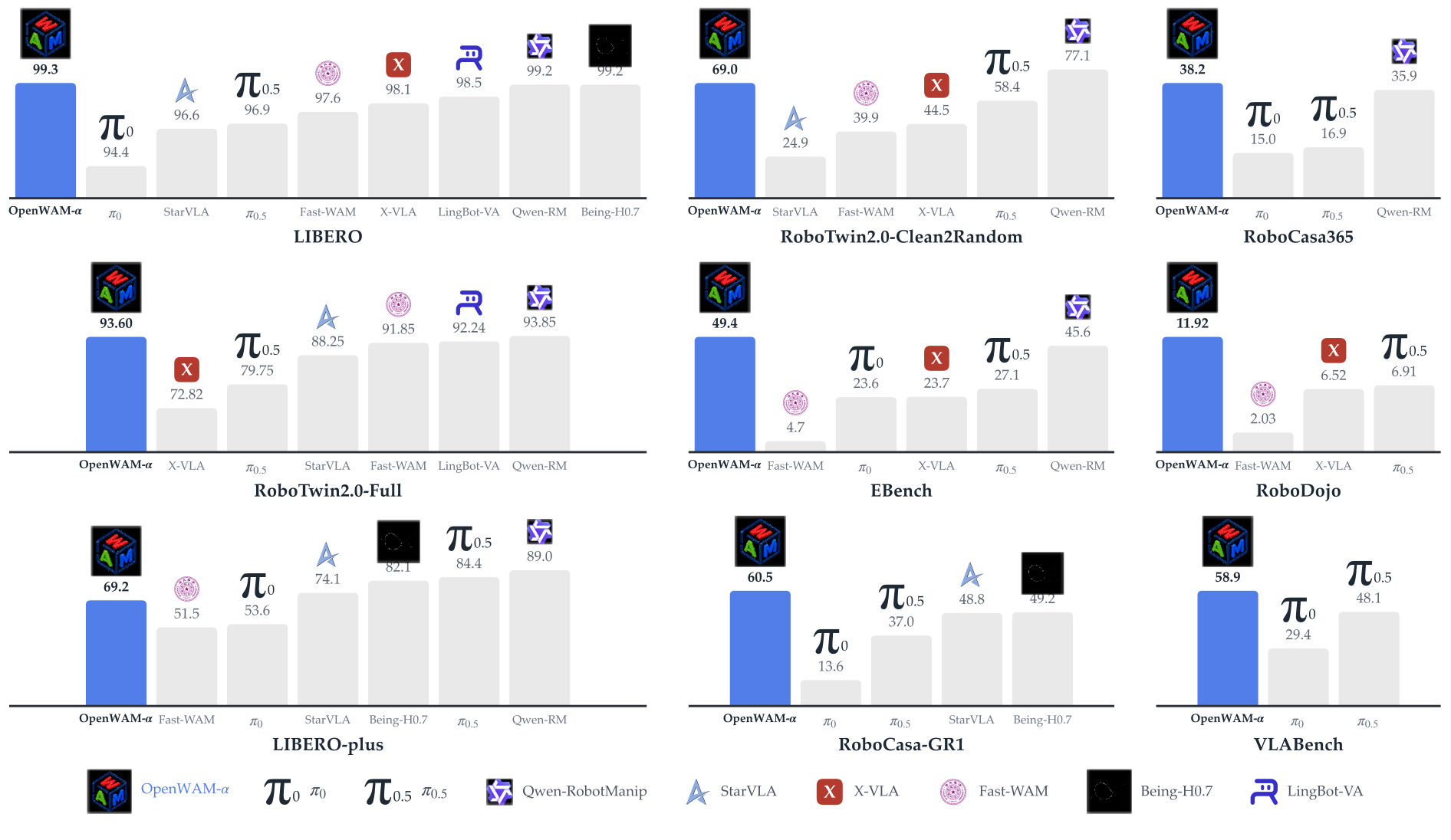
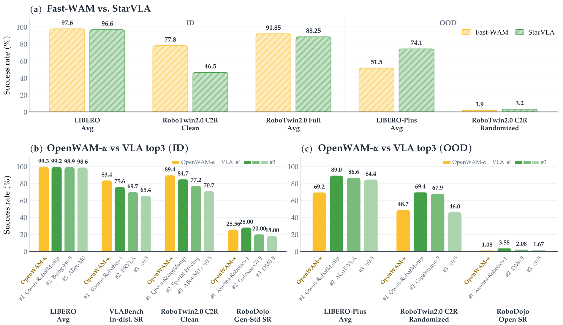
Figure 13 presents representative comparisons; Appendix D preserves all reported baseline rows. Aggregate scores and success rates are not interchangeable, and clean/randomized averages should not be presented as randomized success alone.
5.3.1 Benchmark results
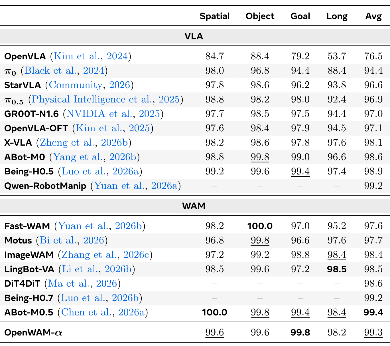
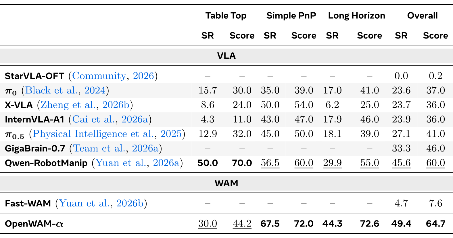
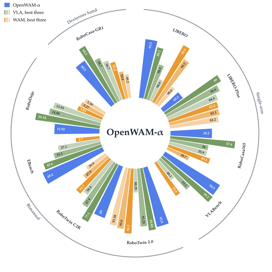
OpenWAM-α achieves 99.3% on LIBERO and 93.6% on RoboTwin-Full, close to reported leaders at 99.4% and 94.1%. It leads the shown EBench aggregate with 49.4% success and 64.7 progress, but loses its tabletop subset to Qwen-RobotManip.
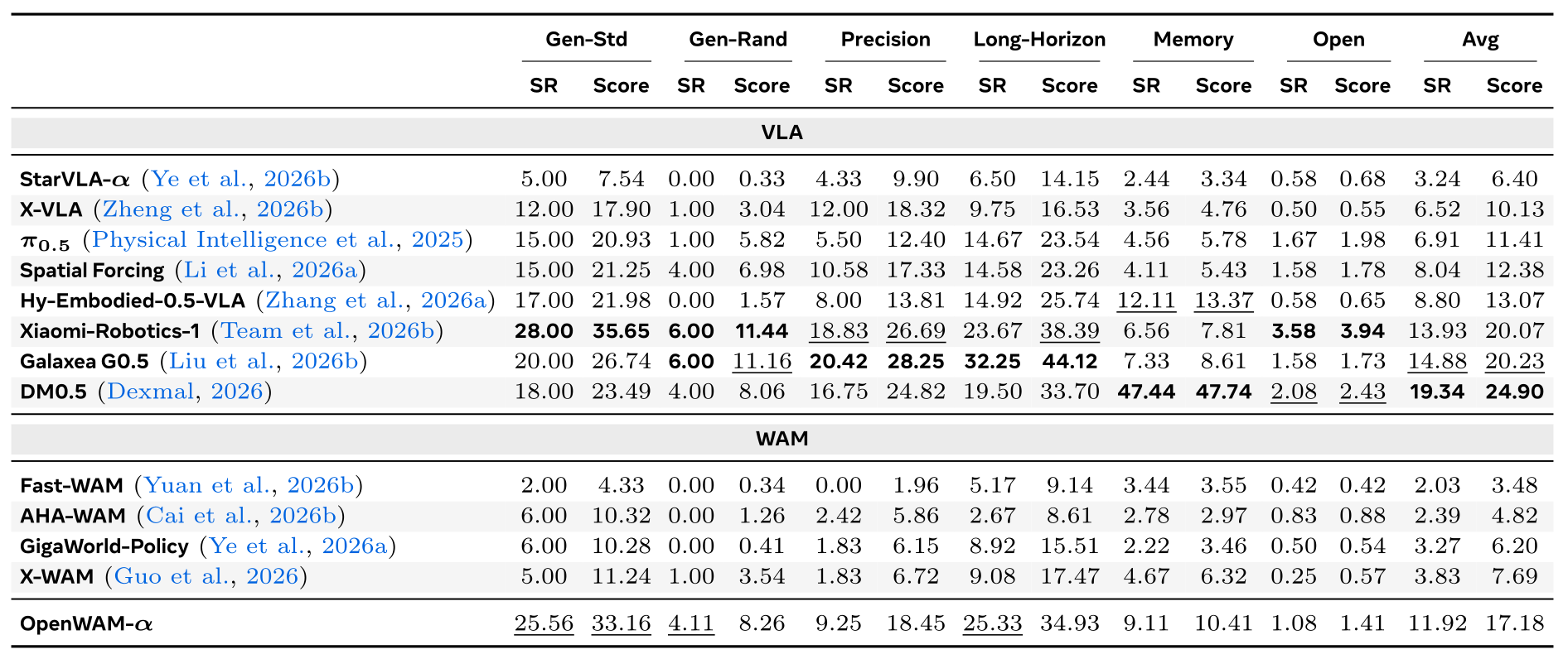
Its RoboTwin-Clean2Random score is 89.4% clean and 48.7% randomized; 69.0% is their average. On RoboDojo, 11.92% success leads the listed world–action models but trails the strongest vision–language–action baseline at 19.34%.
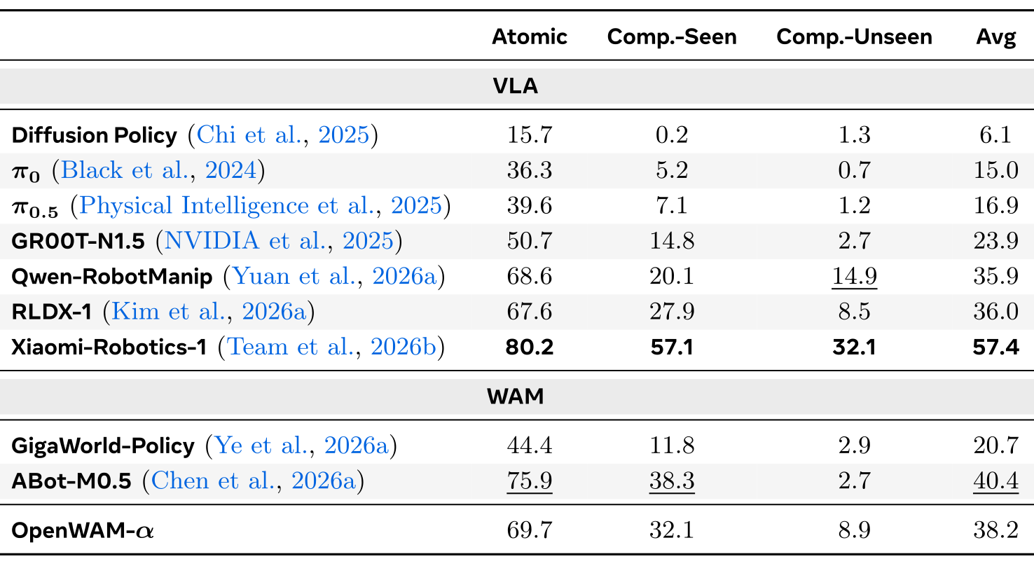
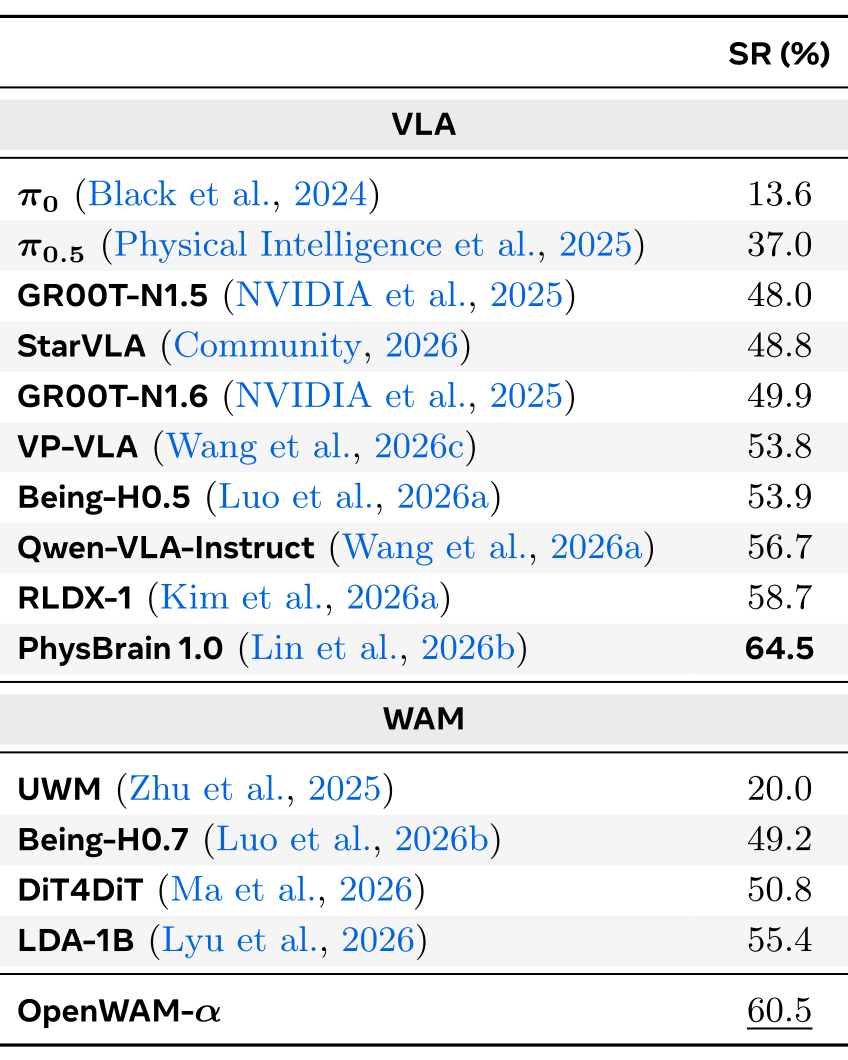
RoboCasa365 is a material exception to the main text’s “marginal gap” description: α averages 38.2% versus the best 57.4%, a 19.2-point gap, and is also below ABot-M0.5 at 40.4%. RoboCasa-GR1 reaches 60.5% versus 64.5%. Table-level evidence supports competitive performance, not uniform leadership.
LIBERO-Plus robustness
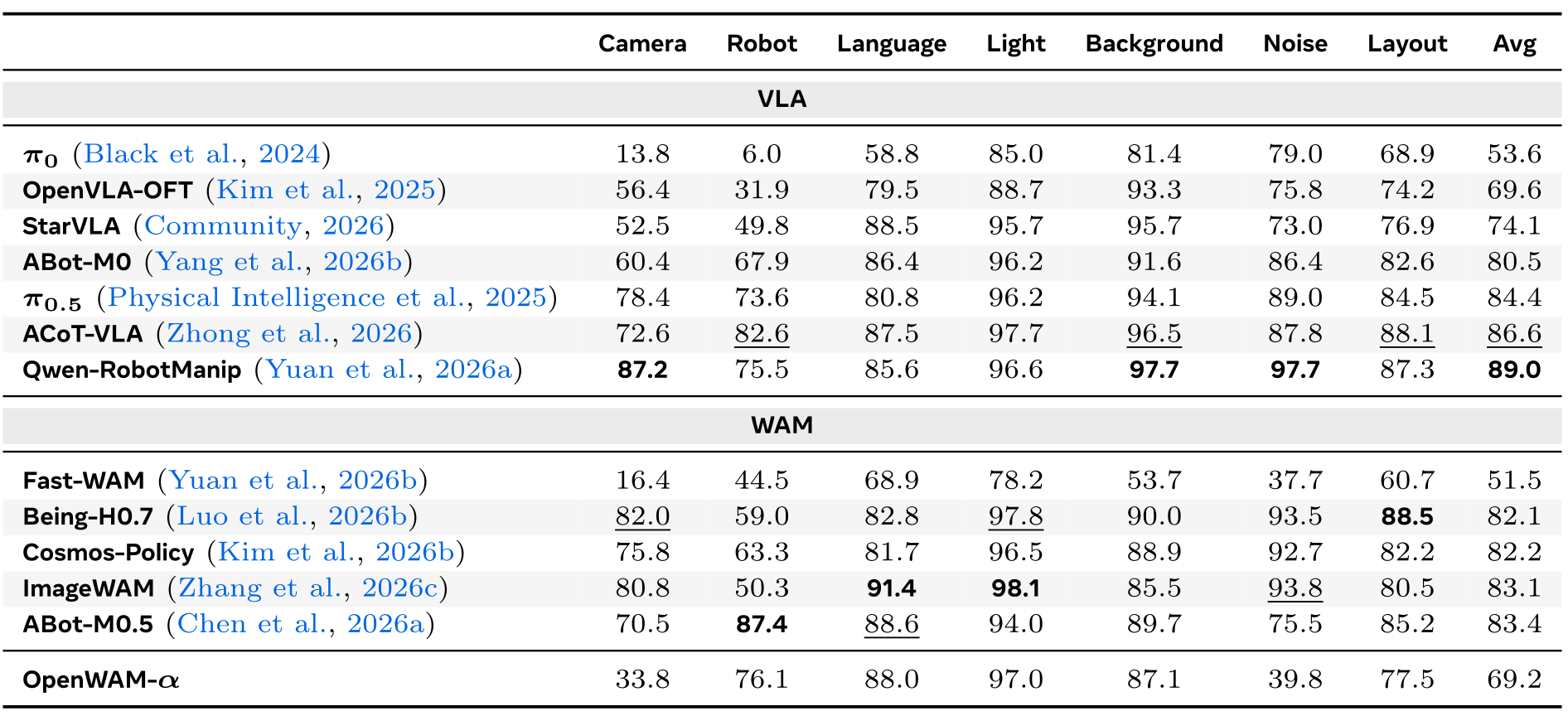
LIBERO-Plus reuses the LIBERO fine-tuned checkpoint. Average success is 69.2%, versus Qwen-RobotManip’s 89.0%. Camera changes score 33.8% and image noise 39.8%, while lighting reaches 97.0%, language 88.0%, and background 87.1%.
The breakdown identifies specific visual robustness gaps; it is more informative than describing all out-of-distribution changes as equally difficult. The full table preserves every perturbation category.
Data and representation diagnoses
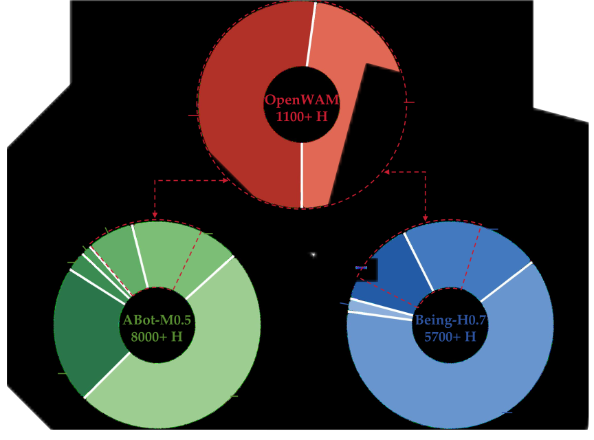
Figure 15 compares roughly 1,100 hours of single-arm pretraining in OpenWAM with over 8,000 in ABot-M0.5 and 5,700 in Being-H0.7. The authors attribute some robustness differences to data diversity and some to pixel-predictive versus semantic representations.
These are cross-model diagnoses with different architectures and data, not isolated causal ablations. The claim that pixel prediction compounds camera/noise errors is a hypothesis consistent with selected comparisons.
Table 4 marks dexterous task coverage for AgiBotWorld-Beta and RoboCOIN. The later adaptation experiment tests a specifically unseen Wuji/Tianji platform and its 9+21-dimensional action layout; it does not establish that pretraining contained no dexterous robot data.
5.3.2 VLA versus WAM
Figure 16 compares models without embodied pretraining and then larger pretrained systems. The observed pattern favors world–action models on several in-distribution splits and vision–language–action models on several shifted splits.
The paper’s broad “neither paradigm prevails” conclusion is reasonable as an empirical summary. It does not prove inherent superiority on either class of task: data coverage, representation, architecture, and optimization differ together, and the per-category tables contain exceptions.
5.4 Real-robot evaluation
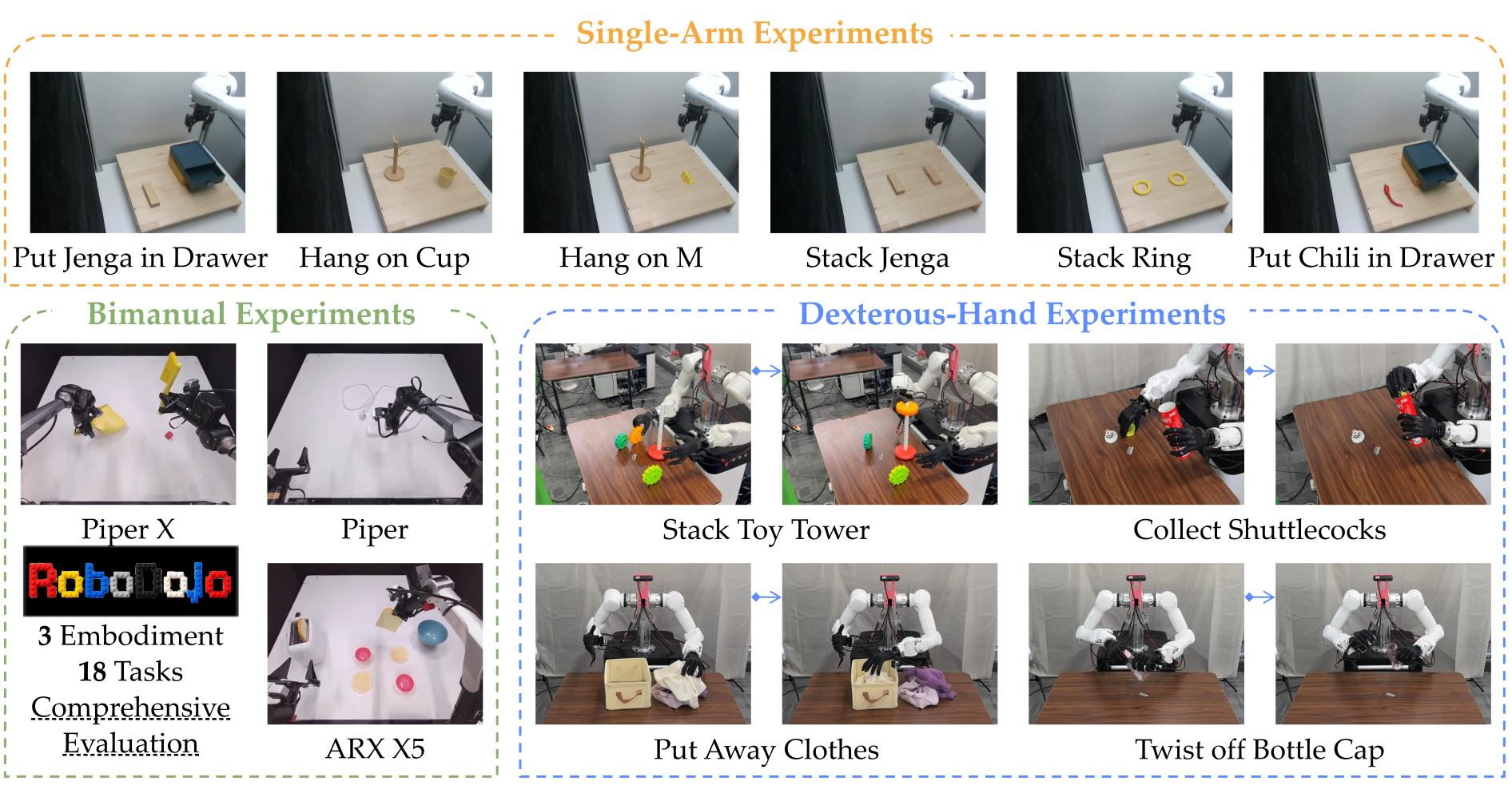
Figure 17 shows six Franka single-arm tasks, 18 RoboDojo bimanual tasks on ARX X5/Piper/Piper X, and four tasks using a Wuji hand with a Tianji arm. All downstream evaluations use fine-tuned policies and distinguish complete success from partial progress where applicable.
Single-arm and bimanual results
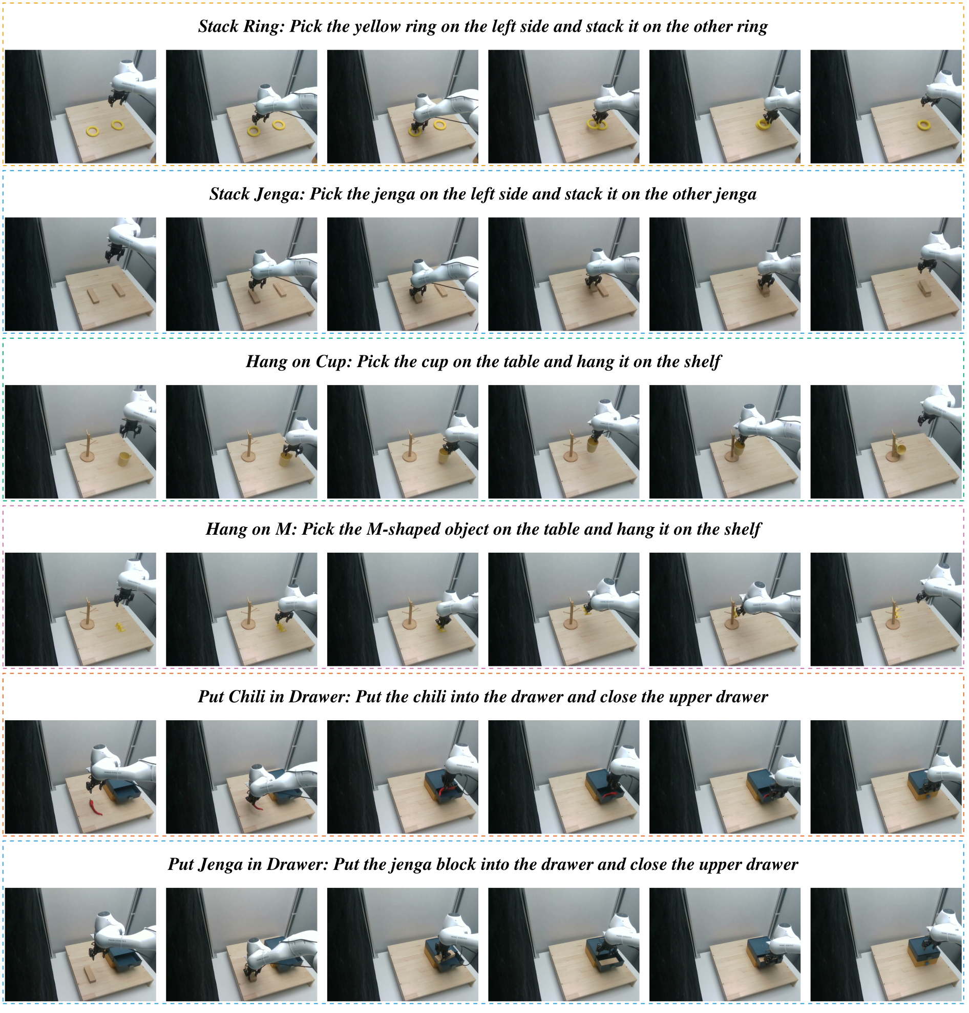
Across 120 single-arm trials, α succeeds in 99 (82.5%), versus LingBot-VA’s 93 (77.5%) and π0.5’s 66 (55%). Against LingBot-VA it wins four tasks, ties hanging the M-shaped object, and loses ring stacking, 60% versus 75%.
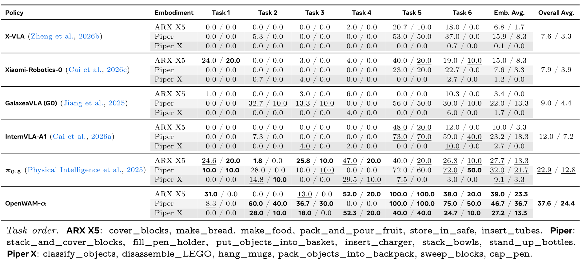
On the 18-task bimanual evaluation, aggregate progress/success is 37.6/24.4 versus π0.5’s 22.9/12.8. Several tasks still have zero success, and some individual success rates are lower despite better partial progress. Table 7 retains the exact task-order key needed to interpret its numbered columns.
The retained project rollouts illustrate selected executions. They are demonstrations, not substitutes for the trial counts or evidence of uniform reliability.

Dexterous-hand adaptation
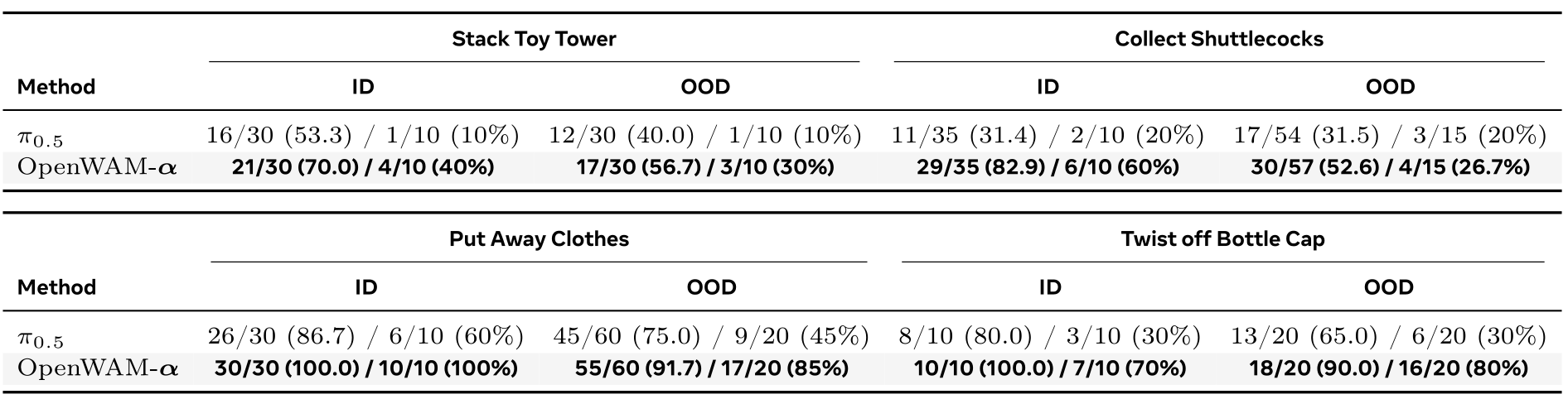
The pretrained model is fine-tuned on a previously unseen 30-dimensional control space: nine end-effector coordinates plus 21 hand degrees of freedom. Table 8 compares four tasks under original and altered conditions. This is adaptation to a new embodiment, not zero-shot dexterous control.
α has higher reported progress and success than π0.5 in every listed task/condition. For example, clothes cleanup reaches 100% in-domain and 85% shifted success, while shifted shuttlecock success remains 4/15, or 26.7%. Small counts and absent confidence intervals limit precision.
Shuttlecock progress uses different shifted object totals, 57 for α and 54 for π0.5. This is an element-weighted score, not a matched per-trial mean. The complete numerators and denominators are retained.
6. Conclusions
OpenWAM contributes a modular implementation, a conditional experimental recipe, and a broadly evaluated pretrained baseline. Its strongest practical lesson is to track representation, data coverage, action supervision, and serving protocol together.
The reported evidence favors several components and shows useful transfer, while leaving substantial robustness and long-horizon gaps. The public infrastructure, checkpoint metadata, data recipe, and full tables make those gaps inspectable.
Acknowledgments
The authors thank Nilaksh and Chuning Zhu for discussions and Wuji Technology for compute resources.
A. Limitations and future work
The study emphasizes embodied pretraining rather than post-training algorithms. Architecture exploration centers on attention and hard-routed experts; early fusion and softly routed experts remain open.
UMI-style and DexUMI robot-executable demonstrations are absent from the mixture [21] [88]. They could connect broad scene diversity with action supervision, but this paper does not test that improvement.
Wan-VAE is a practical compromise, not an established optimal encoder. Compact representations that retain control-relevant information and withstand viewpoint, noise, and scene changes remain a central limitation.
B.1 Pretraining configuration
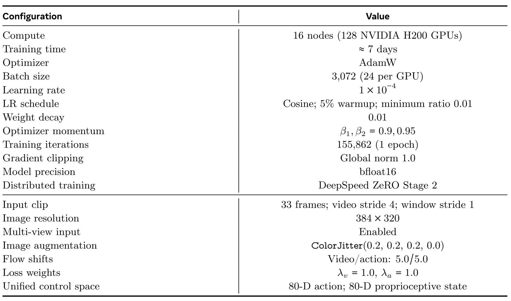
Table 9 retains the complete configuration. Training uses 128 H200 processors for about seven days, 155,862 optimizer steps, one epoch, and batch size 3,072. AdamW uses learning rate 10⁻⁴, cosine decay, 5% warmup, weight decay 0.01, momenta 0.9/0.95, and global gradient clipping at one.
Inputs contain 33 frames with video stride four and window stride one at 384×320 resolution. Training uses bfloat16, ZeRO stage two, multi-view inputs, and ColorJitter(0.2, 0.2, 0.2, 0.0).
B.2 Dataset-specific fine-tuning
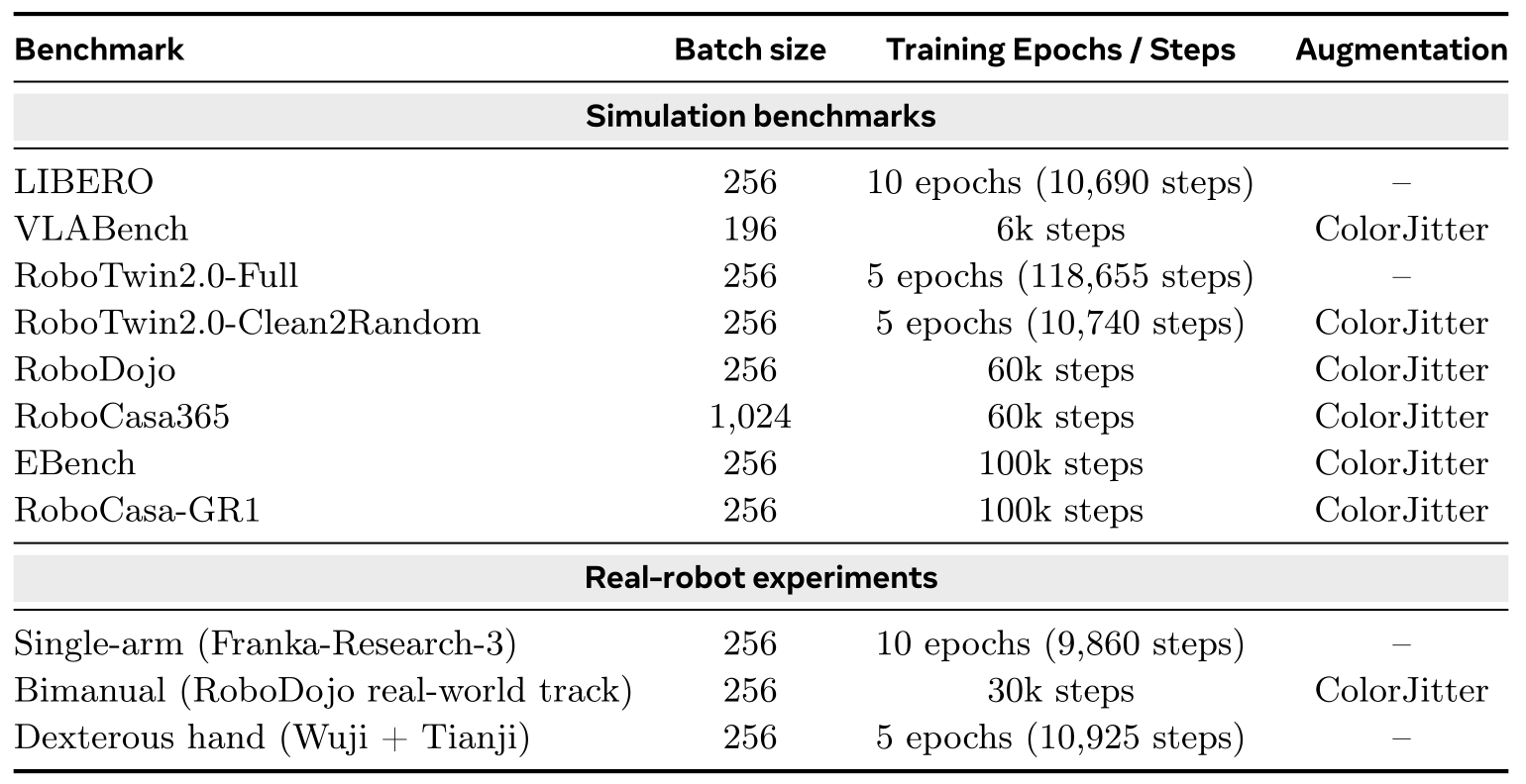
Table 10 preserves every dataset-specific batch size, training duration, and augmentation setting. Most use batch 256; VLABench uses 196 and RoboCasa365 1,024. LIBERO-Plus receives no additional fine-tuning.
Real single-arm training uses 9,860 steps over ten epochs; bimanual training uses 30,000 steps; dexterous adaptation uses 10,925 steps over five epochs. The appendix does not provide the dexterous demonstration count, so epoch counts alone do not specify dataset size.
C.1 Single-arm real-robot protocol
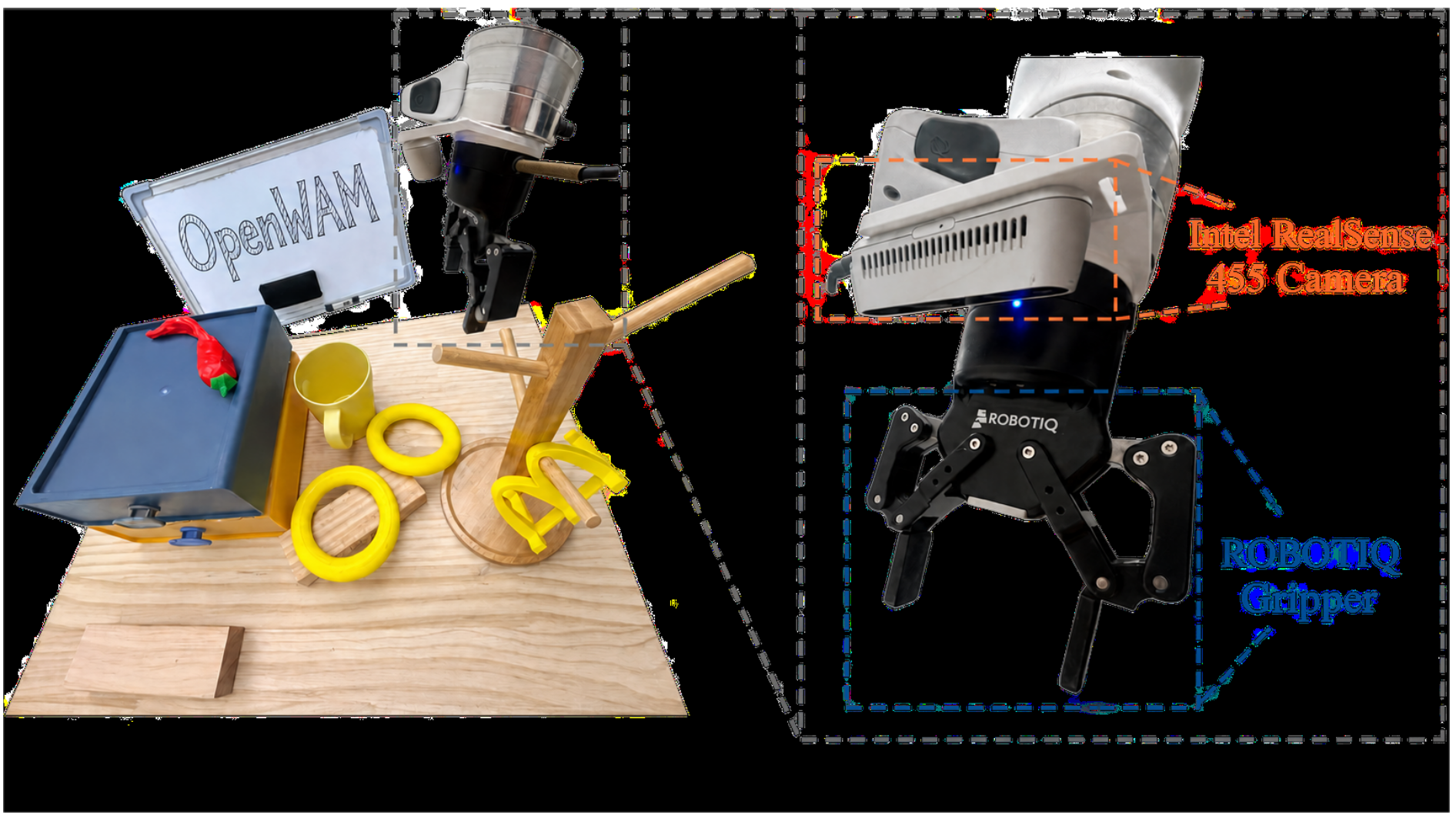
The Franka-Research-3 uses a parallel gripper, camera observations, language, and proprioception. Each of six tasks has 100 demonstrations and 20 independent evaluation trials. Success requires stable placement, maintained hanging, or placing the object in the drawer and closing it, depending on the task.
Table 11 retains every original instruction. Figures 18–19 preserve hardware and six-frame task sequences; the original six project rollout videos are also retained.

C.2 Dexterous-hand protocol
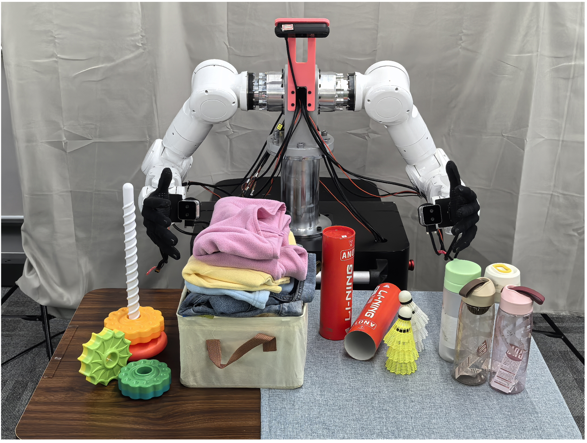
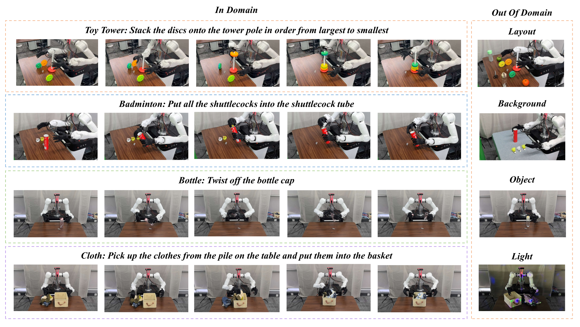
The four tasks stack three discs by size, collect two to four shuttlecocks, clear three to four clothing items, or unscrew a bottle cap. Table 12 preserves the exact language instructions; Figures 20–21 retain the platform, task stages, and altered scenes.
Each shifted condition changes one factor, such as object identity, placement, lighting, or background, while preserving the objective. Results do not establish robustness to arbitrary simultaneous combinations. Original project videos retain their individual condition labels.

Success, progress, and task criteria
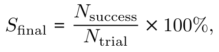
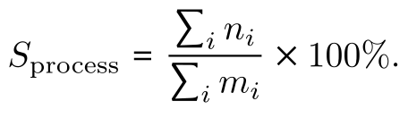
Complete success is the fraction of trials meeting the full objective. Progress divides total completed elements by total available elements across trials, so trials with more objects carry more weight. Both original formulas are preserved.
For tower, shuttlecock, and clothing tasks, partial progress counts placed objects. For the bottle, progress records cap removal; complete success additionally requires maintaining a stable grasp of the bottle or cap. A 100% progress score therefore need not imply 100% successful trials.
Equations
C.3 Bimanual real-robot protocol
The study evaluates all 18 tasks on the official RoboDojo real-robot platforms and follows the benchmark’s task definitions. Table 7 includes the six ordered tasks for each embodiment. The three-platform aggregate does not imply that every task generalizes to every robot without adaptation.
D. Complete simulation results
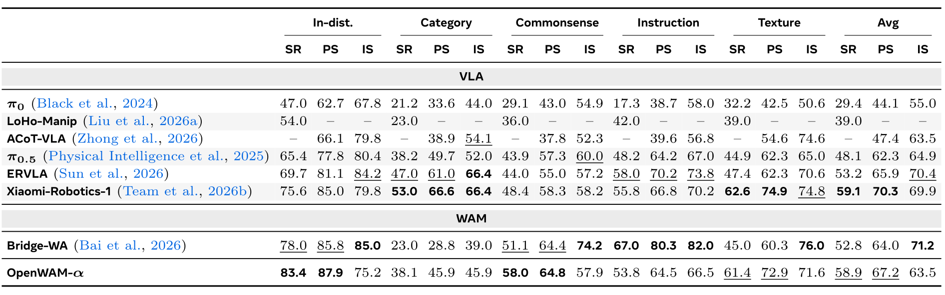
Tables 13–20 retain all simulation results, grouped by model family with the original bold/underline ranking conventions. LIBERO-Plus is retained separately as Table 5.
VLABench reaches 58.9% overall success versus the best 59.1%, but its other metrics and category scores are not uniformly strongest. RoboCasa365 scores 69.7% on atomic tasks, 32.1% on seen composites, and 8.9% on unseen composites. RoboDojo memory success is 9.11% versus the strongest listed 47.44%.
These detailed outcomes qualify the overview charts: high aggregate performance can coexist with weak category transfer, incomplete long-horizon execution, and substantial gaps to a specialist or differently trained baseline.