Overview
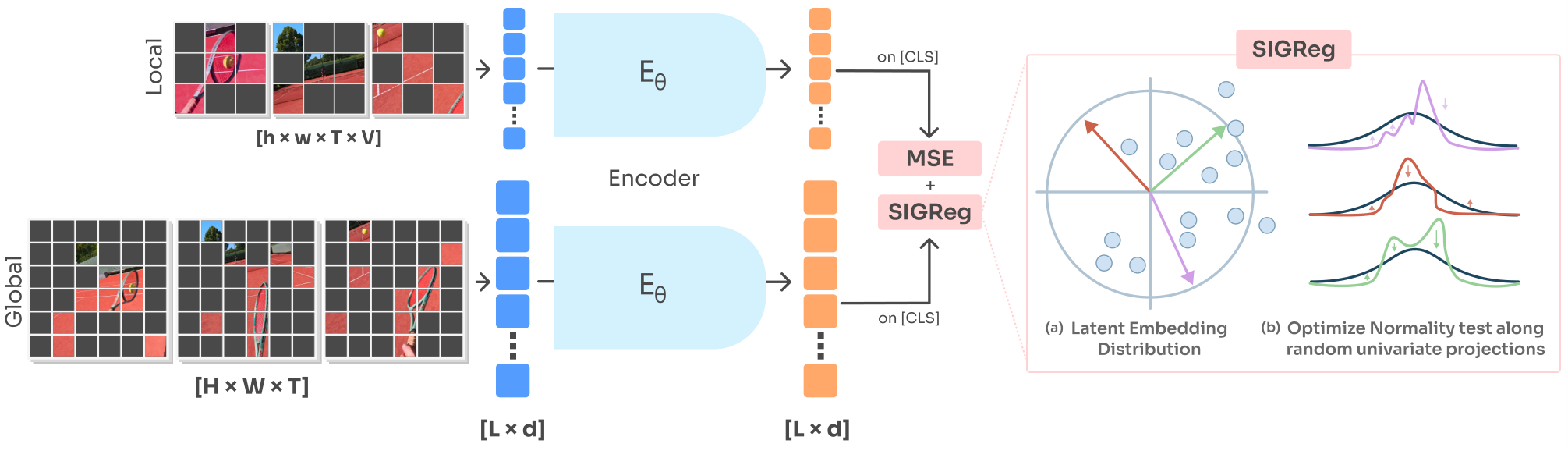
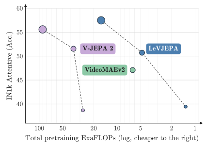
LeVJEPA learns a video representation by making different views of one clip agree while keeping the batch of embeddings spread out like a Gaussian cloud. One shared encoder and a projector replace the teacher–predictor machinery of V-JEPA. Dropping 95% of training patch tokens makes the computation much cheaper. The main evidence is controlled frozen-feature recognition, rather than action-conditioned planning or prediction of a future clip.
1 Introduction
Think of the engineering change as simplifying the training graph before scaling it. Instead of spending computation on a full-clip teacher and masked-token predictor, LeVJEPA processes small random samples of each view with the same network. Its experiments separate equal-epoch comparisons from equal-compute comparisons. Block-causal patch attention also supports representations that use only observations up to the current frame; this property alone does not supply an action-conditioned dynamics model.
2 Related Work
The closest ingredients come from two branches of self-supervised learning: matching multiple views and explicitly controlling the distribution of their embeddings. LeVJEPA combines those ingredients for video. This changes the purpose of masking: dropped tokens are absent observations, rather than reconstruction targets. The distinction explains why a mask useful for VideoMAE or V-JEPA need not be useful here.
Self-supervised learning from images.
BYOL and DINO learn agreement between augmented views using a teacher–student arrangement; DINO also contributes the global/local crop design. I-JEPA predicts masked-region features. LeVJEPA borrows the multiple-view construction while removing the separate target encoder and predictor, so the resemblance in names should not hide the different training computation.
Explicit constraints on the embedding distribution.
A constant output would make all views agree perfectly. Variance–covariance methods oppose that collapse through feature statistics; LeJEPA instead encourages a specified Gaussian distribution. Its theoretical justification concerns a particular downstream-probe setting and assumptions. Applying that objective to video motivates this method; it does not guarantee good recognition of every action or object.
Pixel reconstruction from video.
VideoMAE must recover missing pixels, so masking the same spatial region through time prevents easy copying from adjacent frames. LeVJEPA never reconstructs those missing values. Keeping only a few randomly scattered observations can therefore be useful without preserving the structured tubes required by the reconstruction task.
Feature prediction and video world models.
V-JEPA predicts feature targets from a momentum encoder. V-JEPA 2-AC subsequently learns action-conditioned dynamics over frozen features for robot planning. LeVJEPA puts temporal causality into its encoder during pretraining, but does not run a robot-planning evaluation here. A causal representation is a possible input to a world model, rather than a complete demonstrated controller.
3 Methodology: LeVJEPA
For one 16-frame clip, make a full spatial view and several cropped, color-augmented views of the same time window. Each goes through one shared video transformer. A small projector maps the clip-level token into the space used by the loss. The projector lets training shape a Gaussian embedding distribution despite layer normalization at the encoder output; downstream evaluation discards it.
Equation 1
| (1) |
3.1 Training Objective
The objective adds two forces: bring representations of the same clip together, and prevent all clips from landing at the same point. The scalar weight balances these terms. Calling this a single-hyperparameter objective refers to that loss weight; optimizer, sampling, architecture and schedule choices still exist.
Invariance.
The mean squared error pulls every local-view embedding toward the global-view embedding. Both sides receive gradients through the same encoder: the global view is a target because of its wider content, not because it comes from a frozen teacher. This term alone admits a constant representation, which is why the distributional regularizer is essential.
Equation 2
| (2) |
Regularization.
Imagine shining many random one-dimensional lights through the embedding cloud. SIGReg checks whether each projected shadow looks like a standard Gaussian, using characteristic functions: averages of bounded complex waves. Matching every possible projection characterizes the full Gaussian distribution. Training uses finitely many directions and numerical integration, so the population theorem should be distinguished from the finite-batch implementation.
Equation 3
| (3) |
3.2 Architecture
Each default token describes one 16×16 patch in one frame. During training, only 5% of patch tokens survive; the clip token always survives. Patch tokens can attend within their frame and to earlier frames, while the clip token reads all observed patches and cannot feed information back into them. Thus per-frame patch features are causal, while the clip readout summarizes the observed clip. Weight averaging supplies only the evaluation checkpoint.
3.3 Pretraining Data and Evaluation Setup
Most comparisons retrain models on the same restricted video corpus, then freeze their encoders and train task-specific readouts. This is a useful control on data and compute, but it measures what a trained probe can extract. It is different from testing an unadapted model, fine-tuning the full encoder, or comparing with each method’s largest publicly released checkpoint.
Pretraining.
The default corpus is a class-balanced 20% subset of K710, with validation overlap removed. A separate scaling experiment adds the full K710 mix, Something-Something-v 2, Walking Tours and PE video data. Treat that larger-corpus result as evidence of additional-data benefit, rather than part of the matched-subset baseline comparison.
Evaluation.
ImageNet probes appearance, Something-Something-v 2 emphasizes motion, and Kinetics-400 measures action recognition. ImageNet and Something-Something use a trained attention readout over frozen features; Kinetics uses mean pooling and a linear classifier. These readouts have different flexibility, so compare methods within each benchmark and protocol rather than comparing raw percentages across tasks.
4 What Matters for Efficient Video Pretraining?
The ablations ask which design choices remain useful once the objective stops reconstructing masked content. They vary token sparsity, the number of local crops, temporal patching and attention direction. The resulting recipe is cheap, but the experiments also reveal a tradeoff: sparse views can hide the cross-frame correspondences needed to recognize motion.
4.1 Token Dropping Improves Representations
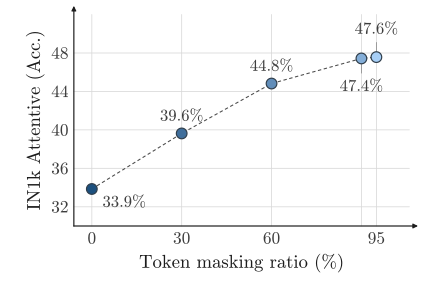
On ImageNet, increasing token dropping from none to 95% raises accuracy from 33.9% to 47.6% in the reported sweep. Dropping therefore acts as an augmentation as well as a compute saving. Motion recognition behaves differently at short schedules and needs longer training to recover. Uniform random locations also outperform repeated spatial tubes, which would hide the same parts of the scene throughout the clip.
4.2 Local View Budget
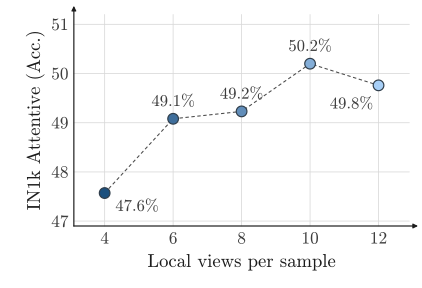
More local views give the network additional partial observations that must agree with the global view. The sweep improves from 47.6% with four locals to 50.2% with ten, then levels off. Each extra crop adds work, so the default uses four; the equal-compute extended run explicitly uses ten. Keep those settings separate when interpreting the results.
4.3 Temporal Patch Aggregation Is Not Required
Combining pairs of frames into one input token saves sequence length but can discard useful temporal detail. Here, per-frame patches win after matching the number of retained training tokens. Evaluation also matches token counts by using eight input frames for per-frame patches versus sixteen for two-frame patches. Equal token counts therefore do not imply equal temporal coverage.
4.4 Causal Attention Incurs No Accuracy Penalty
In the reported ImageNet ablation, block-causal attention scores 51.2% versus 50.7% for bidirectional attention. That supports retaining temporal order without a measured loss on this probe. It does not establish equality on all tasks or quantify end-to-end streaming latency; a deployed cache still needs an appropriate implementation.
| Attention | IN1K top-1 |
|---|---|
| Bidirectional | 50.7 |
| Block-causal | 51.2 |
5 Comparison with Prior Work
Separate three questions: how well models learn after the same number of epochs, what they achieve with the same total training FLOPs, and how video compares with image pretraining on the same source footage. Each comparison fixes a different resource. The headline efficiency claim should be read together with those controls and the task-specific results.
5.1 Comparison to Video Models
At 240 matched epochs on the same 20% K710 subset, LeVJEPA reaches similar or better ImageNet probe accuracy than retrained V-JEPA 2 across the tested model sizes while using 5.6–20.8 times less pretraining computation. These are estimated FLOP savings for the stated recipes, not measured wall-clock speedups or a comparison with V-JEPA 2’s full-scale original release.
| Method | IN1K | SSv2 | K400 |
|---|---|---|---|
| VideoMAEv2 | 53.4 | 43.6 | 37.4 |
| V-JEPA 2 | 51.6 | 42.5 | 40.7 |
| LeVJEPA | 61.0 | 40.4 | 44.6 |
FLOP-matched comparison.
With a fixed FLOP budget, the cheaper method can train for longer: this run uses 1,085 epochs and ten local views. It reaches 61.0% on ImageNet and 44.6% on Kinetics-400, ahead of the compared video baselines, but its 40.4% on Something-Something-v 2 trails VideoMAEv 2’s 43.6%. Equal computation yields a tradeoff rather than a win on every benchmark.
5.2 Comparison to Image Models
DINOv 2 is retrained on frames from the same videos at matched compute. It remains ahead on ImageNet, 53.8% versus 50.7%, while LeVJEPA performs better on motion recognition, 30.4% versus 16.9%. This controlled result supports video’s temporal benefit; it does not compare either retrained model with a much larger image-foundation-model training run.
5.3 Pretraining on consumer hardware
A small demonstration trains ViT-Tiny for twelve hours on one 16 GB RTX 5080 using eight Walking Tours videos. Frozen ImageNet accuracy rises from 8.9% to 25.2%. This shows that nontrivial pretraining fits consumer hardware. It does not imply that the main benchmark models or their reported accuracies can be reproduced with that small budget.
5.4 Scaling the Pretraining Data
On the larger mixed-video corpus, a ViT-L/16 trained for 100 epochs reaches 69.5% ImageNet and 55.0% Something-Something-v 2 accuracy in this pinned paper. The improvement suggests that the objective benefits from more varied data. Because the corpus and schedule change together relative to the restricted runs, this is not a controlled estimate of a universal scaling law.
5.5 Emergent Token-Level Structure
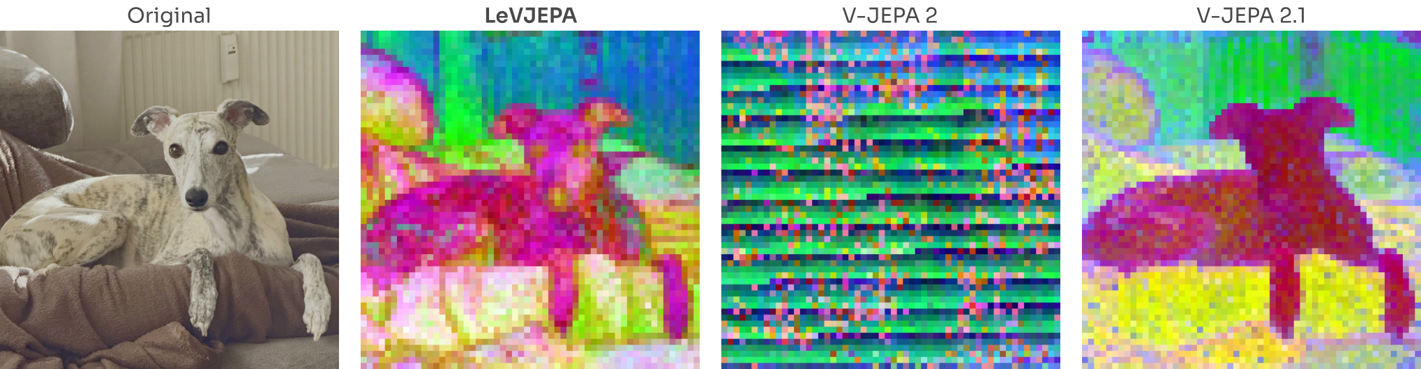
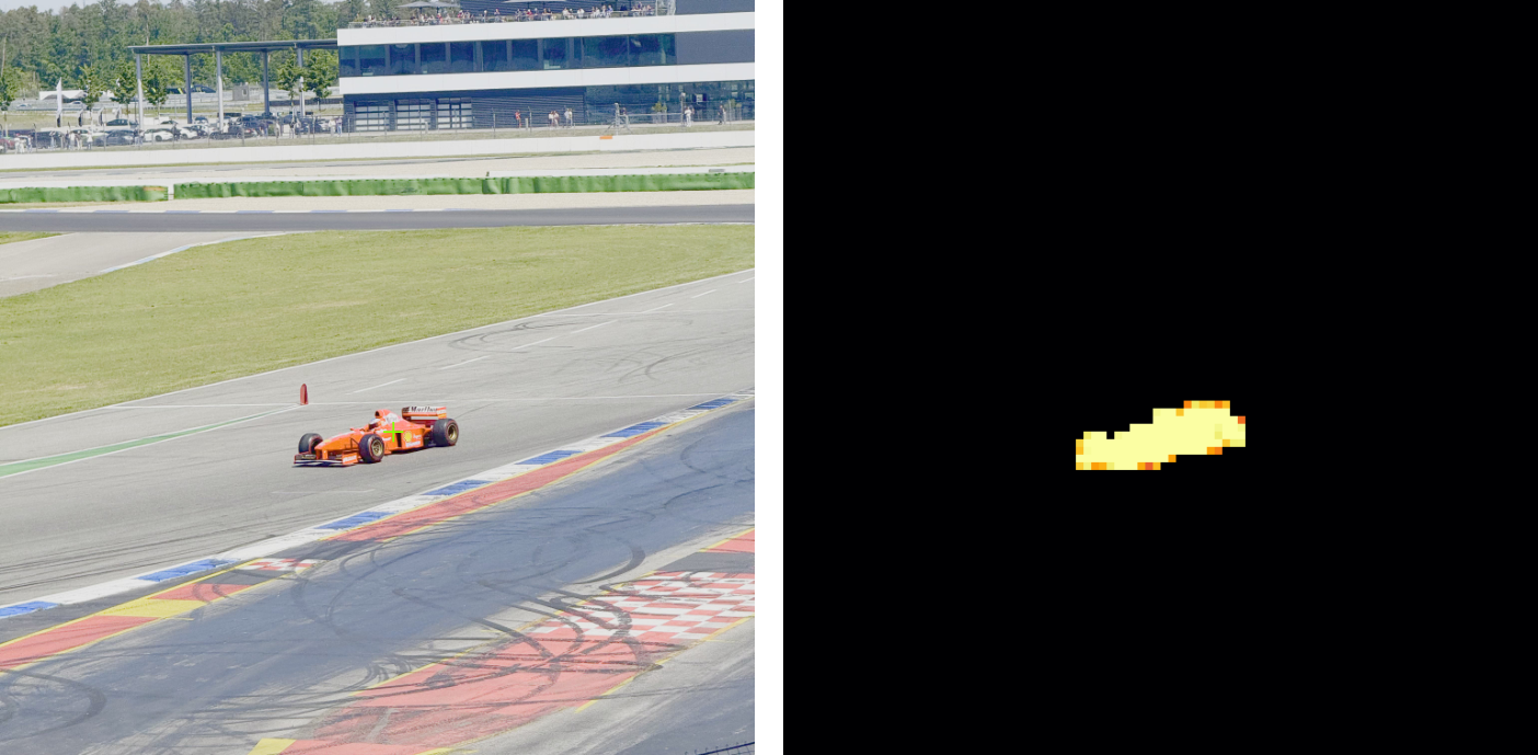
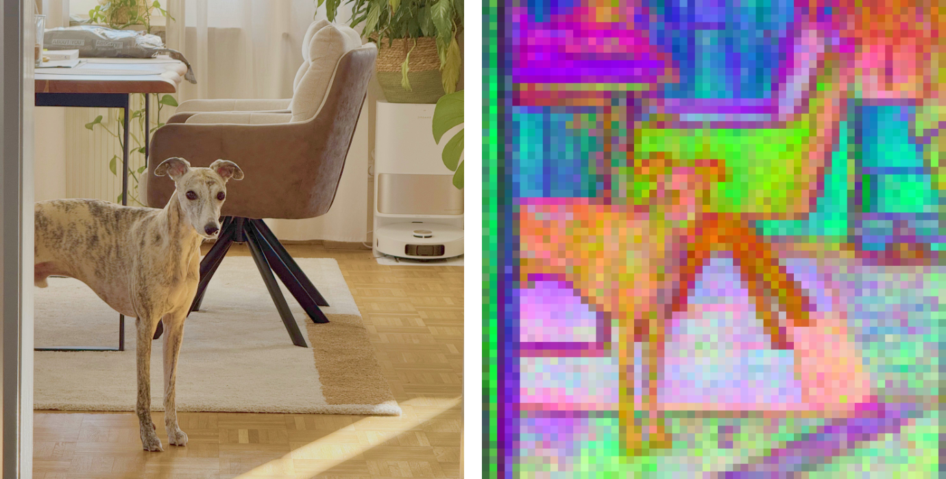
Although only the clip token receives the loss directly, patch-feature visualizations separate some objects from backgrounds. Principal-component colors and query-patch similarities make this emergent structure visible. These examples are qualitative evidence; segmentation, tracking accuracy and robustness require dedicated quantitative tests that the paper leaves open.
6 Discussion
The paper’s strongest engineering result is a simpler, much cheaper recipe for useful frozen video features under controlled comparisons. Its main limits are motion loss at high sparsity, experiments below internet-scale foundation-model training, and qualitative rather than benchmarked dense features. A causal encoder offers a starting point for streaming and future world-model work; this paper does not establish action-conditioned forecasting or safe planning.
Acknowledgments
The original acknowledgments identify institutional and grant support. They describe funding and author responsibilities rather than additional experiments or evidence for the method.
Appendix A SIGReg Implementation Details
The implementation samples 1,024 projection directions and approximates each one-dimensional integral with 17 grid points. Workers average the characteristic-function values before computing the statistic, so regularization sees the global batch. Communication is a small tensor of size 2×1,024×17 rather than all embeddings; finite sampling still approximates the ideal distributional constraint.
Appendix B Architectural Details
The appendix specifies three-coordinate rotary positions and a two-layer projector with 256 output dimensions. It also clarifies an easy terminology trap: encoder weights are Polyak-averaged for evaluation, with no extra forward pass or target branch in the loss. The method removes the training teacher network, rather than forbidding all forms of weight averaging.
Appendix C Evaluation Details
The encoder remains fixed while each downstream readout learns from labeled task data. These appendix details define exactly what the reported representation quality means. Keep the attentive readout for ImageNet and Something-Something separate from Kinetics-400’s mean-pooled linear readout.
Attentive probing.
A learned query attends to all encoder output tokens, and a small residual MLP and classifier produce the label. Only this readout is trained. Because attention and the MLP can combine features nonlinearly, good attentive-probe accuracy does not imply that every class was already separated by a linear boundary in the frozen feature space.
Linear probing on Kinetics-400.
For Kinetics-400, average the frozen output tokens and train one linear classifier. This cheaper readout evaluates a more restricted use of the representation than the learned attention probe used for the other two benchmarks.