GaussVLA: Geometry-Aware Spatial Reasoning for Vision-Language-Action Model

Overview

GaussVLA

At a glance

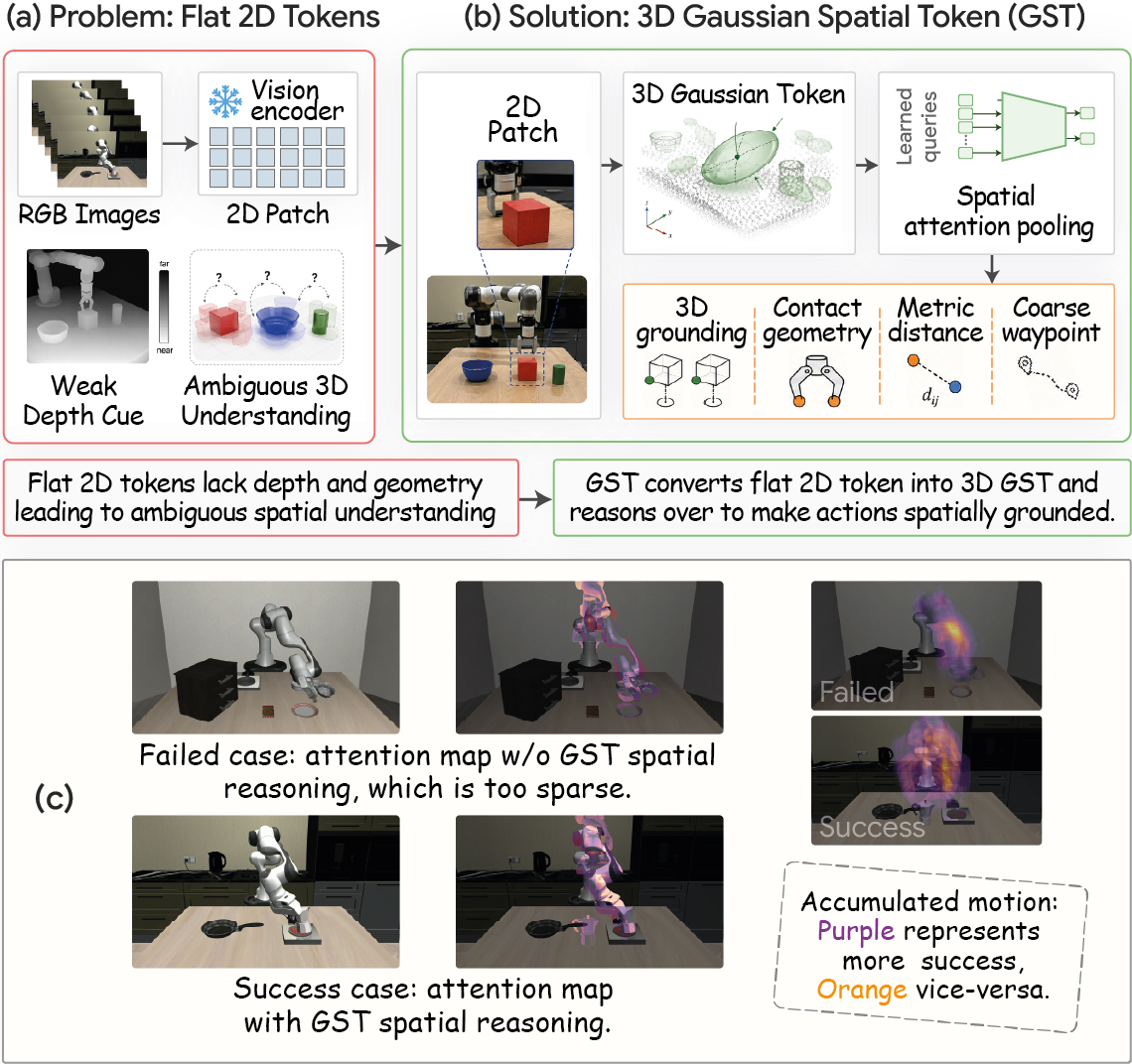
GaussVLA gives robot policies a compact representation of 3D geometry. GST turns image features and estimated depth into Gaussian spatial tokens; DA-CoT uses a few parallel reasoning queries to condition a Mamba-based action policy.

The paper reports 93.5% average success on LIBERO, including 100% on its Spatial suite. Geometry contributes most of the improvement. The reported 200M model parameters exclude frozen external encoders; 179M parameters are trainable. Distribution shifts and very long task sequences remain difficult.

1 Introduction

Conventional VLA models flatten images into 2D tokens, leaving depth, surface structure, and geometric reliability implicit [13] [42] [4]. Adding scalar depth helps, but does not explicitly represent orientation or confidence [27]. Textual CoT adds reasoning at the cost of sequential decoding [33] [36].

GaussVLA combines structured Gaussian geometry, parallel spatial reasoning, and an efficient Mamba backbone [7]. GST represents each patch with a 3D position, spatial extent, and learned confidence. DA-CoT queries that representation while conditioning action generation on language and flow time.

Refer to caption — Figure 1: Overview of *GaussVLA*.

2 Related Works

Discrete action-token models inherit language grounding but accumulate decoding errors. Diffusion and flow-matching policies generate continuous action chunks, with sampling cost as a trade-off [6] [25] [31] [4] [15]. FAST and PD-VLA reduce decoding overhead [26] [28].

SpatialVLA and 3D-VLA add geometric inputs [27] [39]; ECoT and CoT-VLA add intermediate reasoning [33] [36]. Mamba-style SSMs make sequence processing efficient [7] [10] [17], but their compressed hidden state limits direct access to individual spatial features. GaussVLA combines a Mamba policy with attention over geometry-aware tokens to address this limitation.

3 Proposed Method: GaussVLA

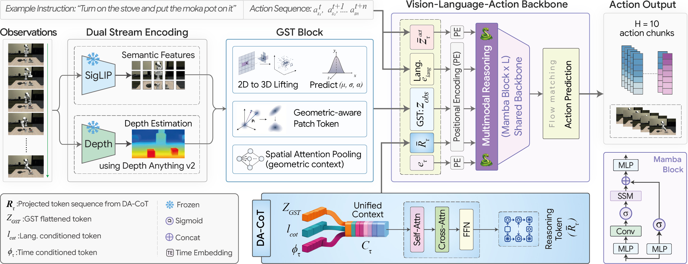
The pipeline is RGB images + instruction → frozen semantic/depth encoders → GST → DA-CoT → Mamba → flow-matching action decoder. The tokenizer supplies geometry, reasoning queries select task-relevant relationships, and the policy generates continuous action chunks.

3.1 Problem Formulation

Training examples pair a window of camera observations and a language instruction with an expert action trajectory. The policy predicts H future actions. Flow matching interpolates between an expert trajectory A and Gaussian noise ε: Zτ = (1 − τ)A + τε, with target velocity ε − A. Observations, language, and flow time condition the predicted velocity.

3.2 Dual-Stream Visual Encoding

Two frozen encoders process the same RGB image: SigLIP supplies patch-level appearance features [34], while Depth Anything V2 estimates depth [32]. Sampling depth at each patch center aligns the two streams. Equations 1–2 define the semantic feature matrix F and corresponding patch-depth vector d.

Equations 1–2

\mathbf{F}_{t}^{(m)}=E_{\mathrm{sem}}(\mathbf{x}_{t}^{(m)})\in\mathbb{R}^{P\times d_{s}},

(1)

\mathbf{d}_{t}^{(m)}=E_{\mathrm{dep}}(\mathbf{x}_{t}^{(m)})\downarrow_{\mathrm{patch}}\in\mathbb{R}^{P},

(2)

3.3 Gaussian Spatial Tokenization (GST)

GST first corrects monocular depth with learned scale and bias, then back-projects each patch through the camera intrinsics (3–4). A semantic-feature head predicts a bounded position correction, log-scale vector, and opacity α (5–7). Fourier-encoded 3D means, semantic features, and log-scales form each geometry-aware token (8–9).

Opacity is learned from semantic features, not directly from a depth-uncertainty estimate. Its reliability interpretation arises through the depth-consistency loss. Spatial pooling uses log α as an attention bias, allowing learned queries to favor more reliable patches (10). The pooled tokens across views and time form the GST representation (11).

Equations 3–11

\tilde{d}_{t,r}^{(m)}=\lambda_{d}\,d_{t,r}^{(m)}+\beta_{d},

(3)

\mathbf{c}_{t,r}^{(m)}=\tilde{d}_{t,r}^{(m)}\bigl(\mathbf{K}^{(m)}\bigr)^{-1}\mathbf{u}_{r}\in\mathbb{R}^{3},

(4)

\left(\Delta\boldsymbol{\mu}_{t,r}^{(m)},\boldsymbol{\eta}_{t,r}^{(m)},\alpha_{t,r}^{(m)}\right)=f_{\mathrm{par}}\!\left(\mathbf{f}_{t,r}^{(m)}\right).

(5)

\boldsymbol{\mu}_{t,r}^{(m)}=\mathbf{c}_{t,r}^{(m)}+\rho\tanh\!\left(\Delta\boldsymbol{\mu}_{t,r}^{(m)}\right),

(6)

\boldsymbol{\sigma}_{t,r}^{(m)}=\exp\!\left(\boldsymbol{\eta}_{t,r}^{(m)}\right).

(7)

\gamma\!\left(\boldsymbol{\mu}_{t,r}^{(m)}\right)=\Big[\sin\!\left(2^{0}\pi\boldsymbol{\mu}_{t,r}^{(m)}\right),\cos\!\left(2^{0}\pi\boldsymbol{\mu}_{t,r}^{(m)}\right),\dots,\sin\!\left(2^{L-1}\pi\boldsymbol{\mu}_{t,r}^{(m)}\right),\cos\!\left(2^{L-1}\pi\boldsymbol{\mu}_{t,r}^{(m)}\right)\Big],

(8)

\mathbf{g}_{t,r}^{(m)}=\left[\mathbf{f}_{t,r}^{(m)}\oplus\gamma\!\left(\boldsymbol{\mu}_{t,r}^{(m)}\right)\oplus\boldsymbol{\eta}_{t,r}^{(m)}\right]\in\mathbb{R}^{d_{g}},\quad d_{g}=d_{s}+6L+3,

(9)

\hat{Z}_{t}^{(m)}=\mathrm{softmax}\!\left(\tfrac{(\mathrm{LN}_{1}(Q)\mathbf{W}_{Q})(\tilde{G}_{t}^{(m)}\mathbf{W}_{K})^{\top}}{\sqrt{d_{p}}}+\mathbf{1}_{N_{g}}\log(\boldsymbol{\alpha}_{t}^{(m)})^{\top}\right)(\tilde{G}_{t}^{(m)}\mathbf{W}_{V}),

(10)

\mathcal{Z}_{\mathrm{GST}}=\left\{\mathbf{z}_{t,j}^{(m)}\right\}_{t=1,m=1,j=1}^{T_{o},M,N_{g}},

(11)

3.4 Depth-Aware Chain-of-Thought (DA-CoT)

DA-CoT flattens the GST tokens and adds projected language and flow-time embeddings (12–13). A small set of learned queries is refined through MHSA, MHCA, and an FFN, with LN and residual updates (14–16).

The result is a compact set of parallel, continuous reasoning tokens conditioned on the current task and flow state. These are intermediate spatial features, rather than a generated natural-language explanation.

Equations 12–16

\bar{Z}_{\mathrm{GST}}=\mathrm{Flatten}\!\left(\mathcal{Z}_{\mathrm{GST}}\right)\in\mathbb{R}^{(T_{o}MN_{g})\times d_{z}},

(12)

\mathcal{C}_{\tau}=\left[f_{\mathrm{gst}}^{\mathrm{cot}}(\bar{Z}_{\mathrm{GST}})\oplus\mathbf{l}_{\mathrm{cot}}^{\top}\oplus\boldsymbol{\phi}_{\tau}^{\top}\right]\in\mathbb{R}^{(T_{o}MN_{g}+2)\times d_{c}}.

(13)

$\displaystyle Y^{(1)}$	$\displaystyle=\mathrm{LN}_{1}\!\left(Y^{(0)}+\mathrm{MHSA}(Y^{(0)})\right),$	(14)
$\displaystyle Y^{(2)}$	$\displaystyle=\mathrm{LN}_{2}\!\left(Y^{(1)}+\mathrm{MHCA}(Y^{(1)},\mathcal{C}_{\tau},\mathcal{C}_{\tau})\right),$	(15)
$\displaystyle R_{\tau}$	$\displaystyle=\mathrm{LN}_{3}\!\left(Y^{(2)}+\mathrm{FFN}(Y^{(2)})\right)\in\mathbb{R}^{N_{r}\times d_{c}},$	(16)

3.5 GaussVLA

Observation, reasoning, language, time, and noisy-action tokens are projected to a shared space and concatenated (17). The Mamba backbone processes the sequence. An action decoder then refines action states using the non-action context and DA-CoT features (18), and a velocity head predicts the flow update (19).

Equations 17–19

\mathbf{Y}_{\tau}=f_{\mathrm{mamba}}\left(\mathbf{e}_{\tau}\oplus\mathbf{e}_{\mathrm{lang}}\oplus\bar{\mathbf{Z}}_{\mathrm{obs}}\oplus\bar{\mathbf{R}}_{\tau}\oplus\bar{\mathbf{Z}}_{\tau}^{\mathrm{act}}\right)\in\mathbb{R}^{(2+T_{\mathrm{GST}}+N_{r}+H)\times d_{b}}.

(17)

\tilde{\mathbf{Y}}^{\mathrm{act}}_{\tau}=f_{\mathrm{dec}}\left(\mathbf{Y}^{\mathrm{act}}_{\tau},\mathbf{Y}^{\mathrm{ctx}}_{\tau},\bar{\mathbf{R}}_{\tau},\mathbf{e}_{\tau}\right)\in\mathbb{R}^{H\times d_{b}}.

(18)

\mathbf{v}_{\theta}=f_{\mathrm{vel}}\left(\tilde{\mathbf{Y}}^{\mathrm{act}}_{\tau}\right)\in\mathbb{R}^{H\times d_{a}}.

(19)

3.6 Training Objectives

Training combines three losses: action flow matching (20), opacity-weighted depth consistency for GST (21), and auxiliary velocity prediction from DA-CoT and action-decoder features (22–24). Their weighted sum is the final objective (25). The DA-CoT target is the action flow velocity; it does not require annotated textual reasoning traces.

Equations 20–25

\mathcal{L}_{\mathrm{FM}}=\mathbb{E}_{(\mathcal{O},s,\mathbf{A})\sim\mathcal{D},\,\tau\sim p(\tau),\,\boldsymbol{\epsilon}\sim\mathcal{N}(\mathbf{0},\mathbf{I})}\left[\left\|v_{\theta}(\mathbf{Z}_{\tau},\mathcal{O},\mathbf{l},\tau)-\mathbf{U}\right\|_{2}^{2}\right].

(20)

\mathcal{L}_{\mathrm{GST}}=\frac{\sum_{t,m,r}\alpha_{t,r}^{(m)}\,\bigl|\mu_{t,r,z}^{(m)}-\tilde{d}_{t,r}^{(m)}\bigr|}{\sum_{t,m,r}\alpha_{t,r}^{(m)}}.

(21)

\bar{\mathbf{r}}_{\tau}=\frac{1}{N_{r}}\sum_{j=1}^{N_{r}}\mathbf{r}_{\tau,j}\in\mathbb{R}^{d_{b}}.

(22)

\hat{\mathbf{U}}_{\mathrm{CoT}}=f_{\mathrm{CoT}}^{\mathrm{res}}\left(\tilde{Y}^{\mathrm{act}}_{\tau}+\mathbf{1}_{H}\bar{\mathbf{r}}_{\tau}^{\top}\right)\in\mathbb{R}^{H\times d_{a}},

(23)

\mathcal{L}_{\mathrm{CoT}}=\frac{1}{Hd_{a}}\left\|\hat{\mathbf{U}}_{\mathrm{CoT}}-\mathbf{U}_{\tau}\right\|_{F}^{2}.

(24)

\mathcal{L}=\mathcal{L}_{\mathrm{FM}}+\mathcal{L}_{\mathrm{GST}}+\mathcal{L}_{\mathrm{CoT}}.

(25)

4 Experiments

4.1 Experimental Setup

Evaluation covers LIBERO [16], LIBERO-PRO [41], Meta-World, CALVIN [22], and a physical SO-101 arm. CALVIN uses the 10% training subset; LIBERO uses 40 rollouts per task. Real-world tasks use 50 demonstrations each.

Frozen SigLIP, Depth Anything V2, and CLIP encoders feed 128 GST queries per camera and four DA-CoT queries. The policy uses five Mamba blocks, hidden size 512, action horizon 10, and ten Euler integration steps. Training uses AdamW, batch size 256, BF16, and auxiliary weights 0.05 and 0.10 with a five-epoch warm-up.

The reported model has 200M parameters, of which 179M are trainable, excluding the frozen external encoders. Latency is 12.97 ms on an RTX Pro 6000 Blackwell. Physical deployment uses a different GPU and 15 Hz control, so these timings should not be conflated.

Method	Venue	Spatial	Object	Goal	Long	Average	Parameters
DP [6]	RSS’23	78.3	92.5	68.3	50.5	72.4	80M
MaIL [10]	CoRL’24	53.8	81.5	56.3	41.7	58.3	24M
QueST [23]	NeurIPS’24	89.0	90.0	88.4	87.0	88.6	152M
OpenVLA [13]	CoRL’24	84.7	88.4	79.2	53.7	76.5	7B
SpatialVLA [27]	RSS’25	88.2	89.9	78.6	55.5	78.1	4B
ThinkAct [8]	NeurIPS’25	88.3	91.4	87.1	70.9	84.4	7B
CoT-VLA [36]	CVPR’25	81.5	91.6	87.6	69.0	82.43	7B
Mask2Act [35]	BMVC’25	76.1	68.7	75.1	30.6	62.6	7B
TraceVLA [40]	ICLR’25	84.6	85.2	75.1	54.1	74.8	4B
$\pi_{0}$ [4]	RSS’26	90.0	86.0	95.0	73.0	86.0	3.3B
SUREFlow[9]	IROS’26	94.8	91.0	93.8	90.2	92.5	179.1M
GaussVLA	BMVC’26	100	95.8	95.3	83.0	93.5	1B

Table 1: Performance comparison on the LIBERO [16] benchmark. GaussVLA achieves the highest overall average success rate while using substantially fewer parameters than large-scale VLA baselines.

4.2 Simulation Results

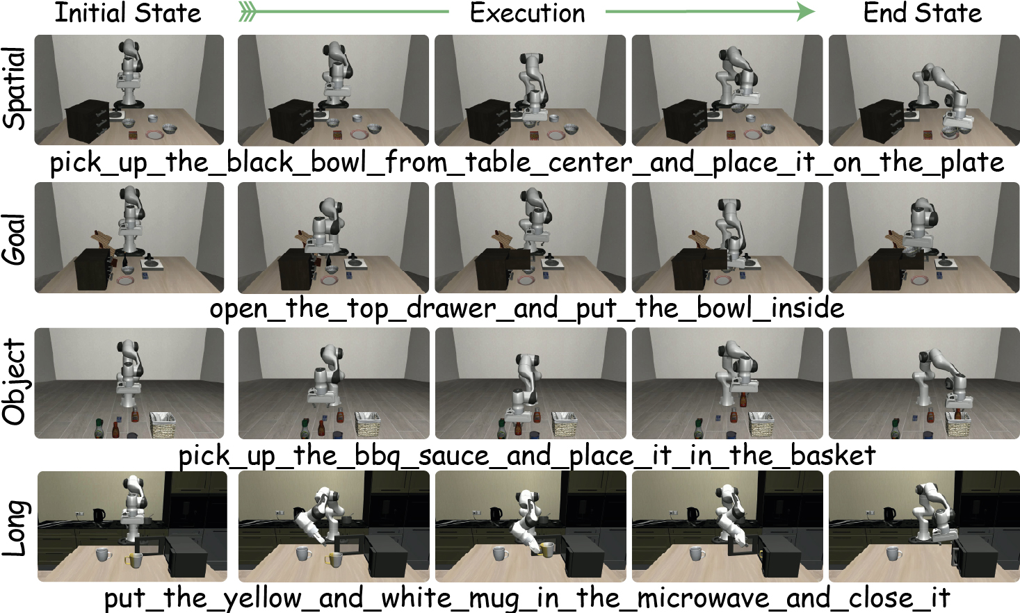
LIBERO: 93.5% average success, 4.9 percentage points above QueST. Suite scores are Spatial 100.0%, Object 95.8%, Goal 95.3%, and Long 83.0%; QueST remains ahead on Long. Table 1 preserves the full comparison.

Beyond LIBERO: GaussVLA has the second-best average on Meta-World among the compared methods. On CALVIN, its mean completed sequence length is 1.474, with GR-1 ahead on one-to-four-task completions and a larger remaining gap at five tasks. These results support spatial manipulation gains while leaving long-horizon recovery unresolved.

Method	Venue	Meta-World					Method	Venue	Tasks completed in a row (CALVIN)					Avg.
Method	Venue	Easy	Mid	Hard	V.Hard	Avg.	Method	Venue	1	2	3	4	5	Length
BC-RNN [19]	CoRL’21	4.5	3.8	3.2	3.0	3.6	MCIL[18]	RSS’21	0.37	0.027	0.002	0.000	0.000	0.40
DP [6]	IJRR’25	83.6	31.1	9.0	26.6	37.6	MT-R3M[24]	CoRL’22	0.408	0.146	0.043	0.014	0.002	0.61
TinyVLA [31]	ICRA’25	77.6	21.5	11.4	15.8	31.6	RT-1[1]	RSS’23	0.249	0.069	0.015	0.006	0.000	0.34
$\pi_{0}$ [4]	RSS’26	71.8	48.2	41.7	30.0	47.9	GR-1[2]	ICLR’24	0.778	0.533	0.332	0.218	0.139	2.0
GaussVLA	BMVC’26	92.7	47.9	37.3	41.6	54.9	GaussVLA	BMVC’26	0.637	0.367	0.291	0.179	0.000	1.474

Table 2: Comparison with recent imitation learning and VLA baselines on Meta-World [21] and CALVIN [22]. The Meta-World panel reports SR across splits by task difficulty. The CALVIN panel reports long-horizon performance as the fraction of rollouts that complete 1-5 consecutive tasks, along with the average length of completed sequences.

Model	LIBERO Goal					LIBERO Spatial					LIBERO 10					LIBERO Object					Avg.
Model	Obj	Pos	Sem	Task	Env	Obj	Pos	Sem	Task	Env	Obj	Pos	Sem	Task	Env	Obj	Pos	Sem	Task	Env	SR $\uparrow$
OVLA [13]	0.96	0.00	0.98	0.00	0.98	0.97	0.00	0.97	0.00	0.89	0.81	0.00	0.96	0.00	0.85	0.98	0.00	0.98	0.00	0.00	0.52
$\pi_{0.5}$ [3]	0.97	0.38	0.97	0.00	0.46	0.97	0.20	0.97	0.01	0.46	0.92	0.08	0.93	0.01	0.46	0.98	0.17	0.96	0.01	0.73	0.53
$\pi_{0}$ [4]	0.94	0.00	0.93	0.00	0.39	0.95	0.00	0.97	0.00	0.60	0.79	0.00	0.82	0.00	0.27	0.94	0.00	0.90	0.00	0.29	0.44
GaussVLA	0.81	0.00	0.70	0.00	0.00	0.93	0.00	0.73	0.00	0.27	0.83	0.00	0.67	0.00	0.00	0.92	0.00	0.63	0.00	0.17	0.33

Table 3: Comparison on LIBERO-PRO [41] benchmark. Normalized success rates (SR) under five perturbation types. Here, OVLA: OpenVLA [13].

4.3 Robustness and Real-World Evaluation

LIBERO-PRO remains difficult: GaussVLA achieves about 0.33 normalized average success and does not lead the benchmark. On the real SO-101 platform, reported multi-task success is 58.8%, versus 46.3% for SpatialVLA and 35.7% for ACT.

Pick-Place success is 81.0% ID and 46.7% OOD. The improvement over SpatialVLA is 12.0 and 10.9 percentage points respectively. The substantial ID–OOD gap remains evidence of sensitivity to distribution shift.

Variant	2D Tokens	GST	DA-CoT	LIBERO $\uparrow$	LIBERO-PRO $\uparrow$	Params (M) $\downarrow$	Trainable (M) $\downarrow$	GFLOPs $\downarrow$	Latency (ms) $\downarrow$
Vanilla GaussVLA	✓	✗	✗	78.1	11.2	179	158	3.50	10.85
+ GST only	✗	✓	✗	90.5	29.0	190.2	169.2	4.33	12.27
+ DA-CoT only	✓	✗	✓	82.1	16.7	188.8	167.8	4.00	11.55
Full GaussVLA	✗	✓	✓	93.5	33.3	200	179	4.83	12.97

Table 4: Core contribution and efficiency ablation. Vanilla GaussVLA denotes the same architecture with GST and DA-CoT removed. GST contributes the dominant performance gain, while DA-CoT provides a complementary improvement. Efficiency is measured on a single NVIDIA RTX Pro 6000 Blackwell. Latency is end-to-end, including frozen encoder forwards and the 10-step Euler ODE of the flow-matching action expert.

$N_{g}$	8	32	64	128	256
LIBERO (%) $\uparrow$	86.4	90.7	92.4	93.5	93.6
Latency (ms) $\downarrow$	11.6	12.0	12.4	12.97	14.1
$N_{r}$	1	2	4	8	16
LIBERO (%) $\uparrow$	91.8	92.8	93.5	93.4	92.9
Latency (ms) $\downarrow$	12.7	12.8	12.97	13.2	13.7

Table 5: Sensitivity to GST queries

N_{g}

and DA-CoT queries

N_{r}

. Default

N_{g}{=}128

,

N_{r}{=}4

is near-optimal on LIBERO and Pareto-optimal on the LIBERO/latency frontier.

4.4 Ablation Study

Removing both modules yields 78.1% LIBERO success. Adding GST alone raises it to 90.5%; DA-CoT alone reaches 82.1%; combining them reaches 93.5%. LIBERO-PRO improves from 11.2% to 33.3% with both modules.

The full model raises latency from 10.85 to 12.97 ms and computation from 3.50 to 4.83 GFLOPs. Query sweeps favor 128 GST queries and four DA-CoT queries: larger settings bring little accuracy benefit while increasing latency. Geometry supplies the larger gain; reasoning adds a complementary benefit.

5 Conclusion

GaussVLA shows that structured geometry can improve a relatively small robot policy. GST contributes most of the measured gain, while DA-CoT improves action conditioning and robustness.

Limitations: severe distribution shifts, viewpoint changes, instruction perturbations, and long-horizon recovery remain challenging. The authors propose stronger camera calibration, viewpoint augmentation, per-episode geometric adaptation, and broader instruction perturbations as future work. Parameter comparisons should retain the exclusion of frozen encoders.

Acknowledgement

This work was supported by the National Research Foundation of Korea(NRF) grant funded by the Korea government(MSIT) (No. IRIS RS-2023-00219725).

Appendix A Additional Implementation Details

The appendix retains the implementation settings, hardware details, representation probes, and additional ablations below.

A.1 Architecture Hyperparameter

Table 6 contains the architecture and training configuration used by default.

GST		DA-CoT
$N_{g}$ Gaussian queries	128	$N_{r}$ reasoning queries	4
Fourier bands $L$ ( $d_{\gamma}{=}6L$ )	10	Reasoning dim $d_{c}$	512
Workspace radius $\rho$	0.8 m
Backbone		Action expert
Mamba blocks $L_{b}$	5	Action horizon $H$	10
Backbone dim $d_{b}$	512	Action dim $d_{a}$	7
Intermediate dim	1024	Flow-matching ODE steps	10
Loss weights (target)		Optimization
$\bar{\lambda}_{\mathrm{GST}}$	0.05	Optimizer	AdamW
$\bar{\lambda}_{\mathrm{CoT}}$	0.10	Learning rate	$2.5{\times}10^{-5}$
Warm-up epochs	5	Weight decay	$1{\times}10^{-4}$
Flow time $p(\tau)$	$\mathrm{Beta}(1.5,1.0)$	Schedule	cosine
		Batch size	256
		Precision	BF16

Table 6: Architecture and training hyperparameters used for all reported GaussVLA runs.

A.2 Real-World Setup

A.2.1 Hardware

Hardware comprises a six-DOF SO-101 arm, parallel-jaw gripper, and RealSense RGB-D camera at 640 × 480 and 60 Hz. Control runs at 15 Hz with horizon-10 replanning. A GeForce 1080 Ti runs inference; the paper’s latency benchmark instead uses an RTX Pro 6000 Blackwell.

A.2.2 Tasks

Tasks are Pick-Place, language-specified Stacking, and left/right Sorting of cubes and a small wheel. OOD Pick-Place changes the camera pose by ±5 cm and ±10° from training positions.

A.2.3 Training

Each task has 50 teleoperated demonstrations. SigLIP and Depth Anything V2 remain frozen.

A.3 Per-Component Latency Breakdown

At batch size one in BF16, frozen image/depth encoders take 8.50 ms; trainable components and ODE integration add 4.47 ms, totaling 12.97 ms. The authors also report an amortized 5.32 ms per control step across action chunks; this differs from the full policy-query time.

Component	Trainable	Latency (ms)
Frozen SigLIP-SO400M/14 forward	✗	5.20
Frozen Depth-Anything-V2 (ViT-L)	✗	3.30
GST module (lift + pool, $N_{g}{=}128$ )	✓	1.42
Mamba backbone	✓	1.50
DA-CoT conditioner	✓	0.70
Action decoder	✓	0.25
Flow-matching ODE (10 Euler steps)	✓	0.60
Total	–	12.97

Table 7: End-to-end inference latency on a single NVIDIA RTX Pro 6000 Blackwell with batch size 1 and BF16 precision. All component latencies sum to 12.97 ms per step.

A.4 Probing the Learned Representations

Linear probes predict object position, gripper–object distance, and orientation more accurately from GST than from flat 2D features. DA-CoT improves these probe scores further. A separate surface-normal probe of GST covariance reaches R² = 0.67 versus a 0.05 random baseline, suggesting learned orientation information without direct normal supervision.

Probe target	Flat 2D patches	Pooled GST	DA-CoT $R_{\tau}$
Object center (3D position)	0.34	0.66	0.78
Gripper–object distance	0.41	0.71	0.82
Object orientation (principal axis)	0.28	0.49	0.61
Surface normal (linear from $\sigma$ )	—	0.67	—

Table 8: Linear-probe regression

R^{2}

on LIBERO simulator state. DA-CoT tokens

R_{\tau}

encode richer 3D geometric structure than flat 2D patch tokens or pooled GST representations.

A.5 Action Decoder Ablation

With GST and DA-CoT disabled, switching from a Transformer to Mamba raises LIBERO success from 67.49% to 73.36% while reducing computation from 9.82 to 3.28 GFLOPs. Adding an action-token query decoder reaches 78.1% at 3.50 GFLOPs. This isolates the backbone/decoder contribution before geometric modules are added.

Backbone	Action Decoder	Query Type	Overall Avg. $\uparrow$	Params (M) $\downarrow$	GFLOPs $\downarrow$
Transformer	Standard head	–	67.49	256	9.82
Mamba	Standard head	–	73.36	110	3.28
Mamba	Action decoder	action-token queries	78.1	179	3.50

Table 9: Overall Avg. is the LIBERO average. The

+4.74

pt jump from row 2 to row 3 jointly reflects the action-token query decoder design and the

+69

M-Parameters/

+0.22

GFLOPs capacity uplift; we hold the Mamba backbone fixed across the comparison to isolate decoder-family effects from backbone-family effects. Here, row 3 (Mamba + Action decoder) corresponds to the Vanilla GaussVLA configuration of Table 4 of the main paper; Adding GST + DA-CoT yields Full GaussVLA at 4.83 GFLOPs (Table 4, main paper).

A.6 GST Ablation

With DA-CoT disabled, simply appending scalar depth lowers overall LIBERO success from 78.1% to 73.3%. Full GST reaches 90.5%, including 100% Spatial success and 29.0% on LIBERO-PRO. The ablation favors structured Gaussian geometry and confidence-aware pooling over raw depth concatenation.

Visual Representation	Depth	3D Lifting	Gaussian Param.	Spatial Pooling	LIBERO $\uparrow$	Spatial Tasks $\uparrow$	PRO Avg. $\uparrow$
Flat 2D patch tokens	✗	✗	✗	✗	78.1	71.2	11.2
2D patch tokens + depth concat	✓	✗	✗	✗	73.3	78.0	14.9
GST tokens	✓	✓	✓	✓	90.5	100	29.0

Table 10: GST design ablation (without DA-CoT). Gains arise from the structured Gaussian representation with confidence-aware pooling, not depth alone: scalar-depth concatenation regresses LIBERO (78.1

\rightarrow

73.3).

A.7 DA-CoT Ablation

With GST disabled, the reported aggregate score increases from 76.7 without reasoning to 83.9 with structured CoT tokens, 85.8 with unsupervised depth-aware reasoning, and 87.0 with full DA-CoT. Depth grounding supplies the larger improvement; auxiliary supervision adds a further benefit. Table 11 preserves the study’s individual metrics.

Reasoning Variant	Depth-Aware	Structured Tokens	CoT Supervision	LIBERO $\uparrow$	Long-Horizon $\uparrow$	Avg. $\uparrow$
No reasoning module	✗	✗	✗	78.1	75.2	76.7
CoT without depth cues	✗	✓	✓	80.5	87.3	83.9
DA-CoT without supervision	✓	✓	✗	81.5	90.0	85.8
DA-CoT (full)	✓	✓	✓	82.1	91.6	87.0

Table 11: Depth-aware grounding is the dominant reasoning ingredient (+3.1 pt on the 2-suite avg, comparing ”CoT without depth cues” 83.9

\rightarrow

”DA-CoT (full)” 87.0). Adding CoT supervision on top of depth-aware structured tokens contributes a complementary boost on both LIBERO (+0.6 pt, 81.5 → 82.1) and Long-Horizon (+1.6 pt, 90.0 → 91.6), for a +1.1 pt 2-suite-avg lift over the no-supervision variant.

A.8 Additional Ablation

Removing the log-opacity attention bias reduces LIBERO success from 93.5% to 91.6% and LIBERO-PRO from 33.3% to 29.7%. Confidence-weighted pooling therefore contributes beyond 3D lifting alone.

Equation 26

\hat{Z}_{t}^{(m)}=\mathrm{softmax}\!\left(\tfrac{(\mathrm{LN}_{1}(Q)\mathbf{W}_{Q})(\tilde{G}_{t}^{(m)}\mathbf{W}_{K})^{\top}}{\sqrt{d_{p}}}+\mathbf{1}_{N_{g}}\log(\boldsymbol{\alpha}_{t}^{(m)})^{\top}\right)(\tilde{G}_{t}^{(m)}\mathbf{W}_{V}),

(26)

A.9 Confidence-Opacity Correlation with Depth-Uncertainty Proxies

The authors compare learned opacity with three independently derived uncertainty proxies on 5,000 LIBERO-Spatial frames: local depth gradients, eight-pass MC-dropout variance, and cross-view photometric inconsistency. Table 12 reports the correlations. These are proxy-based checks, rather than direct ground-truth confidence labels.

Depth-uncertainty proxy	Pearson $\rho(\alpha,-u)$ $\uparrow$	$p$ -value
$u_{\nabla}$ (depth-gradient magnitude)	$+0.61$	$<10^{-6}$
$u_{\sigma_{d}}$ (MC-dropout variance)	$+0.54$	$<10^{-6}$
$u_{\mathrm{pc}}$ (photometric inconsist.)	$+0.47$	$<10^{-6}$

Table 12: Pearson correlation between the learned opacity

\alpha

and three depth-uncertainty proxies (sign convention: higher

\alpha

\Leftrightarrow

lower uncertainty). Although

\alpha

is not directly conditioned on any of these proxies, the opacity-weighted GST loss in Eq. 21 in the main paper induces a strong correlation consistent with the ”depth-aware confidence” interpretation.

A.10 Action-Chunk Horizon Sweep on CALVIN

On CALVIN’s 10% subset, increasing the action horizon from 10 to 20 raises mean completed sequence length from 1.474 to 1.65. Horizon 50 degrades performance. The default remains 10 to preserve frequent replanning and responsiveness, despite the higher benchmark score at 20.

$H$	1	2	3	4	5	Avg. Len.
10 (default)	0.637	0.367	0.291	0.179	0.000	1.474
20	0.671	0.402	0.318	0.198	0.063	1.65
50	0.598	0.331	0.237	0.122	0.030	1.32

Table 13: CALVIN ABCD

\rightarrow

D (10%) performance under varying action-chunk horizon

H

. The default setting

H{=}10

provides a strong trade-off between performance and efficiency.

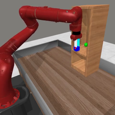
A.11 Meta-World Successful Frames

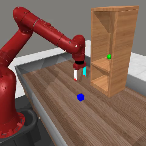
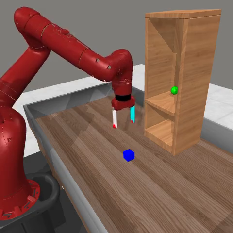
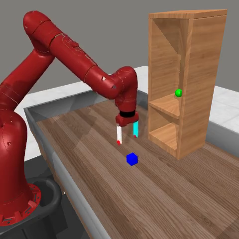
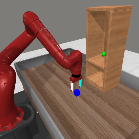
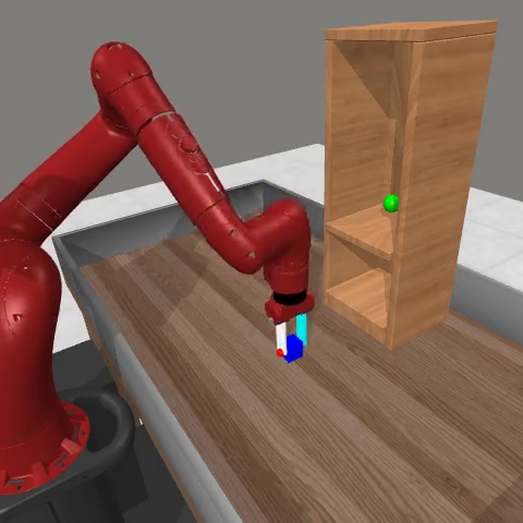
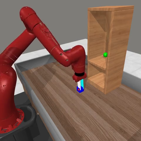
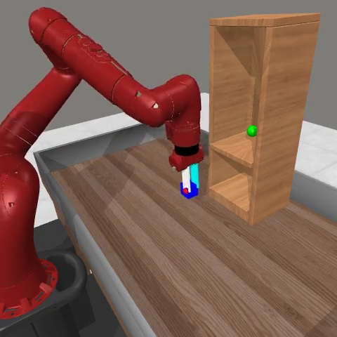
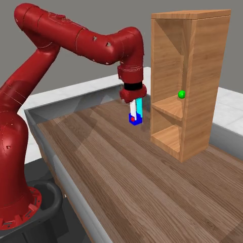
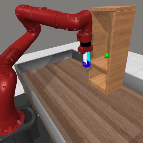
The final figure shows a successful Very Hard Meta-World rollout: approach the object, locate the shelf, grasp the puck, and place it. It is a qualitative example accompanying the benchmark results.