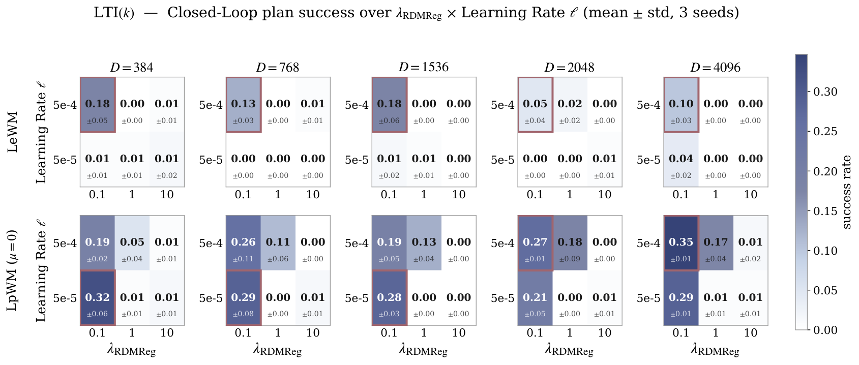
Think of describing a scene with many available features but activating only a few at once. LpWM asks whether these sparse codes make a world model’s job easier. An encoder produces nonnegative features, a predictor forecasts them after an action, and a distribution-matching loss encourages exact zeros without collapsing every observation to the same code. A quantization theorem motivates the idea, but practical learned codes are an approximation to that ideal. In the tested simulations, sparse codes help most when the predictor has intermediate capacity. Which features are active can reveal dynamical regimes, although meaningful contact tracking additionally needs a temporal prior.
1 Introduction
Preventing constant embeddings is necessary for JEPA training, but it does not determine the best representation for predicting motion. Dense Gaussian-like codes are one choice. This paper tests an alternative: use sparse codes so that a simpler predictor may be sufficient, and inspect whether the active-feature pattern reflects how the environment changes.
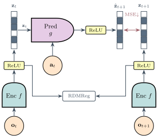
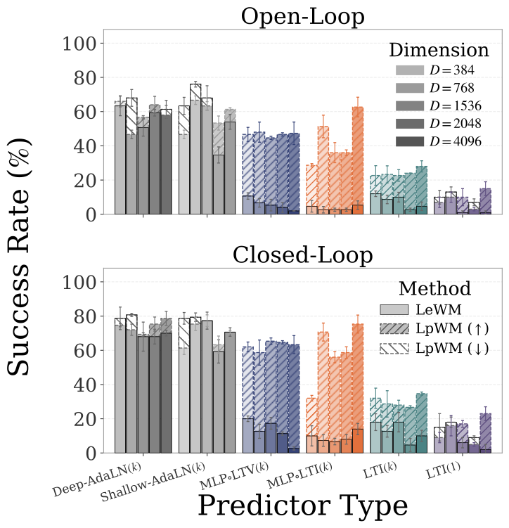
Figure 1: LpWorldModel: a JEPA model with sparse representations. (a) An encoder maps observation to non-negative, sparse latents via a terminal (Rep)ReLU function. The predictor takes inputs and actions to predict , compared against the encoded target . RDMReg (24) matches per-timestep latent marginals to a Rectified Generalized Gaussian, preventing collapse and inducing sparsity. (b). Arrows indicate the success-rate difference between LpWM and LeWM: denotes higher performance for LpWM, while denotes lower performance. LpWM outperforms LeWM with more linear predictor variants (MLPLTV, MLPLTI, and LTI. See full specifications in Table 1) by up to in success rate, while performing on par with LeWM using the high-capacity DiT predictors. This suggests that sparse representations induce a latent space with simpler dynamics to learn compared to their dense counterparts.
Contributions.
The contributions are a sparse action-conditioned world model, an idealized one-hot linearization result, predictor-capacity comparisons, and probes of discrete versus continuous information in the learned code. The theory motivates the experiments; it does not prove that training the practical network reaches the constructed encoding.
2 Method
2.1 LpWM: JEPA with Rectified Distribution Matching Regularization (RDMReg)
Training balances future-feature prediction with a constraint on the feature distribution. Rectified Distribution Matching Regularization compares random one-dimensional projections with samples from a target distribution. Rectification maps negative values to zero, producing nonnegative sparse features; the default target is a rectified Laplace distribution. Matching a finite set of projections is a practical distribution-matching procedure, not an exact finite-sample equality guarantee.
Equations 1–2
(1)
(2)
2.2 Architecture and Rectification
A vision transformer and projection network encode the image; an action-conditioned predictor estimates the next code. The RepReLU link outputs ordinary rectified features but routes gradients through a smoother function. This helps avoid inactive units during optimization. The distribution constraint, rather than this gradient-routing device alone, supplies the anti-collapse mechanism.
Equations
2.3 Planning with the Learned World Model
Encode the current and goal images, imagine candidate action sequences, and score the predicted final feature distance to the goal. The cross-entropy planner repeatedly samples and refines candidate sequences. Closed-loop execution observes the result and replans, so good planning depends on both the learned representation and prediction accuracy.
(a)Support Jaccard Heatmap.
(b)State Decoding.
(c)Planning Evaluation.
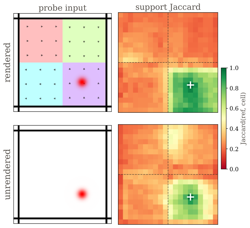
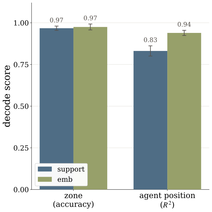
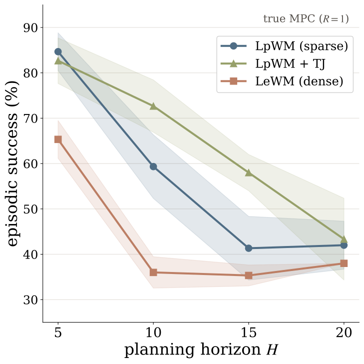
Figure 2: The sparse support recovers the piecewise structure of the dynamics.(a) Support Jaccard heatmap over a grid: the Jaccard index of each cell’s support with a fixed reference cell (white ) is high within the reference zone and drops across zone boundaries (dashed), for a model trained with rendered zones (top) and one with no visual cues (bottom). (b) The binary support decodes the ground-truth zone identity as accurately as the full embedding, while agent position is decoded better from the magnitudes than from the support. (c) Planning success vs. horizon (closed-loop, 3-seed meanstd). Goal locations of the dot agent are sampled randomly. Both sparse variants beat dense LeWM at every horizon.Equation
3 Does Sparsity Simplify Latent Dynamics?
The key experiment varies predictor complexity while holding the representation-learning comparison as consistent as possible. If sparse geometry is easier to predict, its advantage should appear before the predictor becomes powerful enough to solve both versions.
3.1 Linearization of Nonlinear Dynamics with Sparse Representations
Imagine dividing the state space into many tiny cells and representing a state by the identity of its cell. For a fixed action, moving between cell labels is a matrix multiplication on one-hot vectors. Under compactness and Lipschitz assumptions, the decoded approximation becomes accurate as the cells shrink, for a fixed rollout horizon. The matrix depends on the action; this is not a claim of one globally linear system in state and action. Required code size grows exponentially with state dimension.
Proposition 1(Linear Approximation of Nonlinear Dynamics with Sparse Representations).
Let be a compact state space and let
be a compact continuous action space.
Consider a deterministic discrete-time controlled dynamical system where Assume that is uniformly Lipschitz in the state variable, i.e. there exists a
finite constant such that for every and
. Then, for every , there exist 1) a finite latent dimension ; 2) a one-hot sparse encoder ; 3) a decoder ; and 4) an action-conditioned family of matrices such that the latent dynamics are exactly linear in , and the decoded one-step prediction satisfies
Equation 3
(3)
Corollary 1(Sparsity in High-Dimensions).
Let the state space be and consider dividing each coordinate into equal intervals, producing grid cells. We represent each cell by its center with the covering radius . Hence the one-step prediction error satisfies
Equation 4
(4)
For any fixed rollout horizon , and .
3.2 Experiment Designs
Practical models learn distributed sparse codes rather than an infeasibly large one-hot lookup table. Tests compare transformer, state-dependent and fixed linear-core predictors across feature widths, with dense Gaussian and VICReg baselines. Width-dependent parameterization is used to make the capacity comparison more stable. These learned models are empirical relaxations of the theorem.
Table 1: Predictors with Different Levels of Complexity. is the predicted latent, past latents, and the action. AdaLN predictors are Transformer-based models with Adaptive Layer Normalization for action conditioning, i.e. DiT architecture (30). The Deep-AdaLN predictor is the one used in LeWM (28). LTI denotes a linear time-invariant predictor with fixed operators , while LTV denotes a linear time-varying predictor with state-dependent operators . We use MLP to denote one extra nonlinear transform. The history denotes context length, with the single-frame case. The output link is for dense LeWM and for sparse LpWM. See Appendix B for details.
Table 2: Predictor parameter counts across latent dimensions .
Counts are for the predictor alone for each
used in our experiments. LTI, MLPLTI, and MLPLTV are attention-free and far smaller than the AdaLN Transformers.
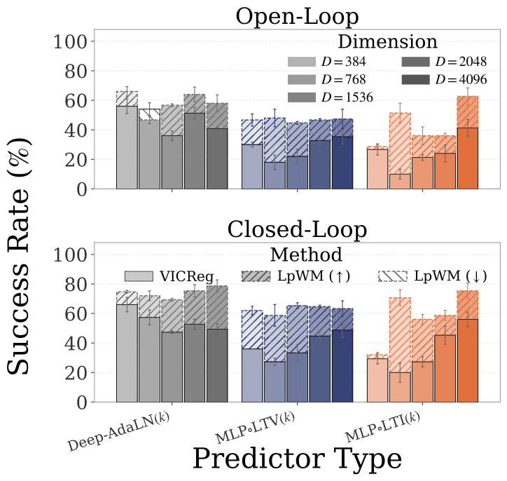
The easy Wall task is already solved by simple predictors for both code types. On PushT, the weakest predictor fails for both, strong predictors reduce the gap, and intermediate-capacity predictors benefit most from sparsity. The result is a capacity-dependent advantage in these settings, rather than a universal ranking of sparse over dense representations.
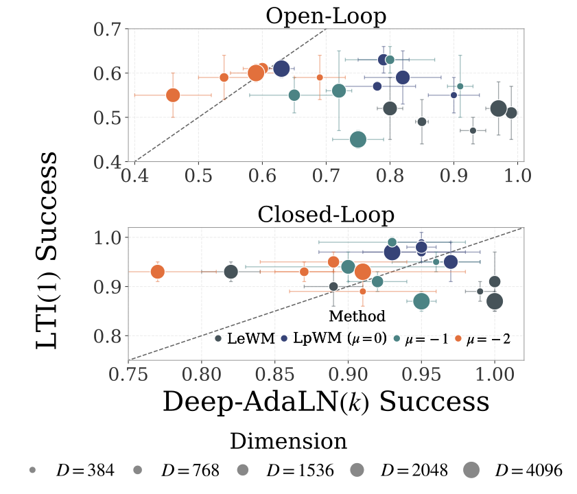
Figure 3: Linear predictor is sufficient for the wall environment regardless of dense or sparse embeddings, and LpWM outperforms VICReg-based JEPA across predictor settings in PushT.(a) We plot the planning success rate of the linear LTI predictor against the nonlinear Deep-AdaLN, where each dot denotes one setting of method and feature dimension. For simplicity, we use to denote LpWM with the target distribution parameter . We show the open-loop evaluation on top and closed-loop results at bottom. Both are ran using CEM planner. We observe that the closed-loop success rate for LTI predictor using SIGReg is already approaching , indicating that the wall environment can already be described well by a linear dynamics model in the latent space. (b) We have already shown LeWM vs. LpWM in Figure 1(b). Here we compare LpWM with a variant of LeWM where we replaced SIGReg with VICReg in the PushT environment across predictor settings. As oppposed to SIGReg, we observe consistent improvement from LpWM over VICReg even for the Deep-AdaLN predictor, and the gap between sparse LpWM and dense methods (i.e. VICReg here) continues to hold for MLPLTV and MLPLTI predictors. See full hyperparameter sweeps in Appendix H.2.
4 Does Sparsity Lead to Interpretable Latent Dynamics?
A sparse representation has two parts: support identifies which coordinates are nonzero; magnitudes describe their values. The paper asks whether support marks discrete regimes while magnitudes retain continuous state within a regime.
(a)Temporal Jaccard Regularization
(b)Example Episode.
(c)Support Raster Plot.
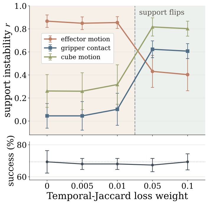
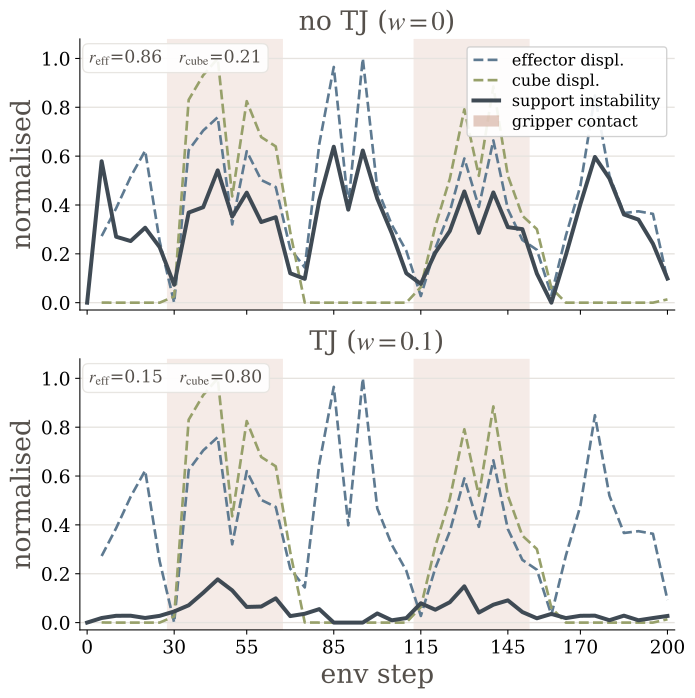
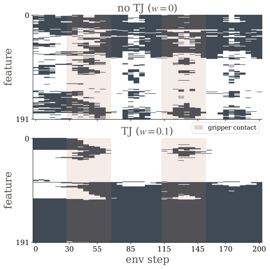
Figure 4: Temporal-Jaccard (TJ) makes the cube support track contact, not effector motion.(a) As TJ strength increases, support-instability correlation with effector motion drops () while cube-motion () and gripper-contact () rise—at no change in planning success. (b) One example episode: without TJ (top) support instability tracks effector displacement (); with TJ (bottom) it tracks cube displacement (), spiking inside the shaded contact windows. (c) Support raster: without TJ the support rapidly transitions across frame; with TJ it is smoothly varying in time, reorganizing almost during the shaded contact window.
4.1 Discovering Piecewise-Affine Dynamics
The controlled Piecewise environment has zones with different force biases. Sparse support identifies those zones even when the background does not reveal them visually; feature magnitudes better recover continuous position. Overlap maps, linear probes and planning tests support this separation in the constructed environment, where the regime labels are known.
Equation 5
(5)
4.2 From Navigation to Contact-Rich Dynamics
On cube manipulation, unregularized support mainly tracks arm movement rather than contact. Adding a temporal Jaccard loss makes the active-feature pattern change more slowly and align better with cube interaction. Sparsity alone therefore does not guarantee a human-meaningful regime decomposition.
5 Conclusion
Sparse feature geometry can reduce the predictor capacity needed for the tested planning tasks. The strongest evidence is the controlled predictor-capacity comparison. Interpretable support is conditional on the environment and temporal constraints; broad conclusions about harder robotics and longer horizons remain open.
Acknowledgement
The authors acknowledge discussions, research support and computing resources that supported the experiments.
Appendix A Related Work
Latent world models for planning.
Latent world models plan by predicting encoded observations rather than reconstructing every pixel. Frozen-feature and jointly trained encoders make different representation-learning choices; this paper focuses on controlling geometry during joint training.
Feature Regularization for Latent World Models.
Anti-collapse methods constrain representation variation or match a target distribution. Their geometry can affect the later dynamics problem. The sparse-versus-dense comparison concerns that geometry as well as the prediction objective.
Sparse and Discrete Representations in World Models.
Sparse and discrete codes restrict which latent patterns are available. LpWM uses distributed nonnegative sparsity, which differs from assigning each observation one discrete token or one-hot identity.
Linearizing Nonlinear Dynamics.
Lifting a nonlinear system into a larger representation can simplify its dynamics. The theorem uses finite state-space quantization; the learned sparse representation is motivated by this idea without inheriting its exact construction or guaranteed accuracy.
Table 3: Sparsity of the LpWM encoder representations across predictor types and latent dimensions. Each entry is the fraction of non-zero coordinates in the sparse code for the target distribution with , measured on the validation set at the tuned-best cell for the LpWM run paired with each predictor at latent dimension . Dense LeWM has active fraction by construction. The learned code stays – active regardless of predictor or dimension, confirming the codes underlying the planning comparison are genuinely sparse.
Table 4: Success Rate (%) over 50 Test Samples in the Piecewise Environments with Varying Numbers of Zones. Piecewise () denotes the environment with varying numbers of zones. Goal images are either sampled from the evaluation dataset or randomly sampled from all possible locations of the dot agent. denotes the horizon and represents the receding-horizon. Results are shown as meanstd over 3 seeds. Bold denotes the best performance.
The predictor ladder ranges from several transformer blocks to fixed linear state-space maps, sometimes followed by a nonlinear readout. The sparse models also retain a rectifying output link, so even a nominally linear predictor need not be an entirely linear end-to-end dynamics model.
A state-dependent gate adds low-rank corrections to fixed transition matrices. This supplies some local flexibility without generating a full matrix with a cubic parameter cost. The action enters the dynamics core affinely, before the shared nonlinear readout. Zero-initialized corrections start from the simpler fixed-operator model.
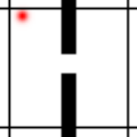
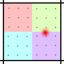
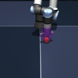
Figure 5: Environments.(a) Wall: 2D navigation through a doorway (red agent). (b) PushT: push a T-shaped block to a target pose (green). (c) Piecewise: an open room partitioned into force-field zones (colored) with a known ground-truth segmentation. (d)OGBench-Cube: a robot arm manipulating a cube.Equation
TwoRoom, PushT and cube-manipulation experiments reuse the cited datasets. Goal images are generally selected 25 raw steps ahead, with five-action blocks. Those choices define relatively short-horizon planning tests.
C.2 Piecewise
Piecewise.
Piecewise divides an otherwise open room into zones, each adding a different motion bias. The resulting dynamics are simple within a zone but change across boundaries. Because the true zones and motion rule are known, the experiment can directly test whether the learned support recovers them.
Equations
C.3 Visualization of Environments
The original environment snapshots are retained. A version without colored zone backgrounds checks whether regime-sensitive features can emerge without an obvious visual label for each zone.
Appendix D Experimental Details
Two pipelines study different questions: predictor complexity on Wall/PushT, and support interpretation on Piecewise/cube manipulation. They share the LpWM objective but differ in architecture and training. Comparisons should be made within their respective pipeline, using the retained configuration table.
Table 5: Experimental configurations for Section 3 and Section 4.
We list out the experimental pipelines in the following table.
The cross-entropy planner uses 300 candidate sequences, keeps 30, and performs 30 refinement iterations. A five-step planning horizon with frameskip five reaches 25 raw steps. Closed-loop tests replan after each action block; open-loop tests execute one plan. Short cube horizons can saturate performance, limiting what those results establish about difficult long-horizon manipulation.
Appendix E Jaccard Index
E.1 Hard and Soft Jaccard index
Jaccard similarity measures the fraction of active coordinates shared by two supports, relative to the coordinates active in either. A continuous relaxation replaces set operations with elementwise minimum and maximum, allowing a differentiable overlap loss for nonnegative codes.
Equations 7
(7)
E.2 Temporal Jaccard Loss
Matching the sparse distribution separately at each time does not specify how support should evolve. The optional temporal loss penalizes rapid changes between neighboring frames. It adds a preference for stable support; it does not itself identify which physical events should define a regime.
Equation 8
(8)
Appendix F Maximal-Update Parameterization ( μ P) for JEPA
Maximum-update parameterization rescales initialization and learning rates as feature width changes. The goal is stable feature learning across capacities, rather than proving that one tuned learning rate always transfers. The authors report occasional transfer exceptions and use explicit sweeps.
Equations 9–10
(9)
(10)
Appendix G Proofs of Linearization
G.1 Proof of Proposition 1
The proof covers the compact state space by finitely many small cells, encodes each representative with one active coordinate, and defines each action’s transition matrix by the representative’s next cell. The error combines the original quantization error, Lipschitz propagation and quantization of the next state. Repeating this argument gives the finite-horizon bound. Original proposition, lemma and equations are retained.
Equations 11–23
(11)
(12)
(13)
(14)
(15)
(16)
(17)
(18)
(19)
(20)
(21)
(22)
(23)
Lemma 1(Finite-horizon rollout bound).
Under the assumptions of Proposition 1, let for be the ground-truth trajectory under an arbitrary action sequence
. Initialize and recursively define the latent transition as
Let be the decoded state.
Then
Equation 24
(24)
Equations 25–30
(25)
(26)
(27)
(28)
(29)
(30)
G.2 Proof of Corollary 1
For a uniform grid on a bounded cube, increasing the number of cells reduces their radius and therefore the approximation error at any fixed horizon. In high dimensions, obtaining small cells needs exponentially many codes—the curse of dimensionality acknowledged by the paper.
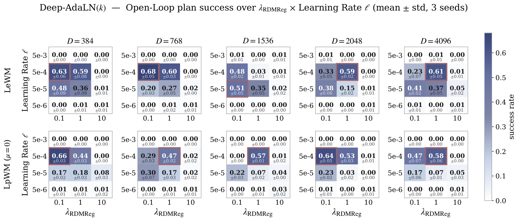
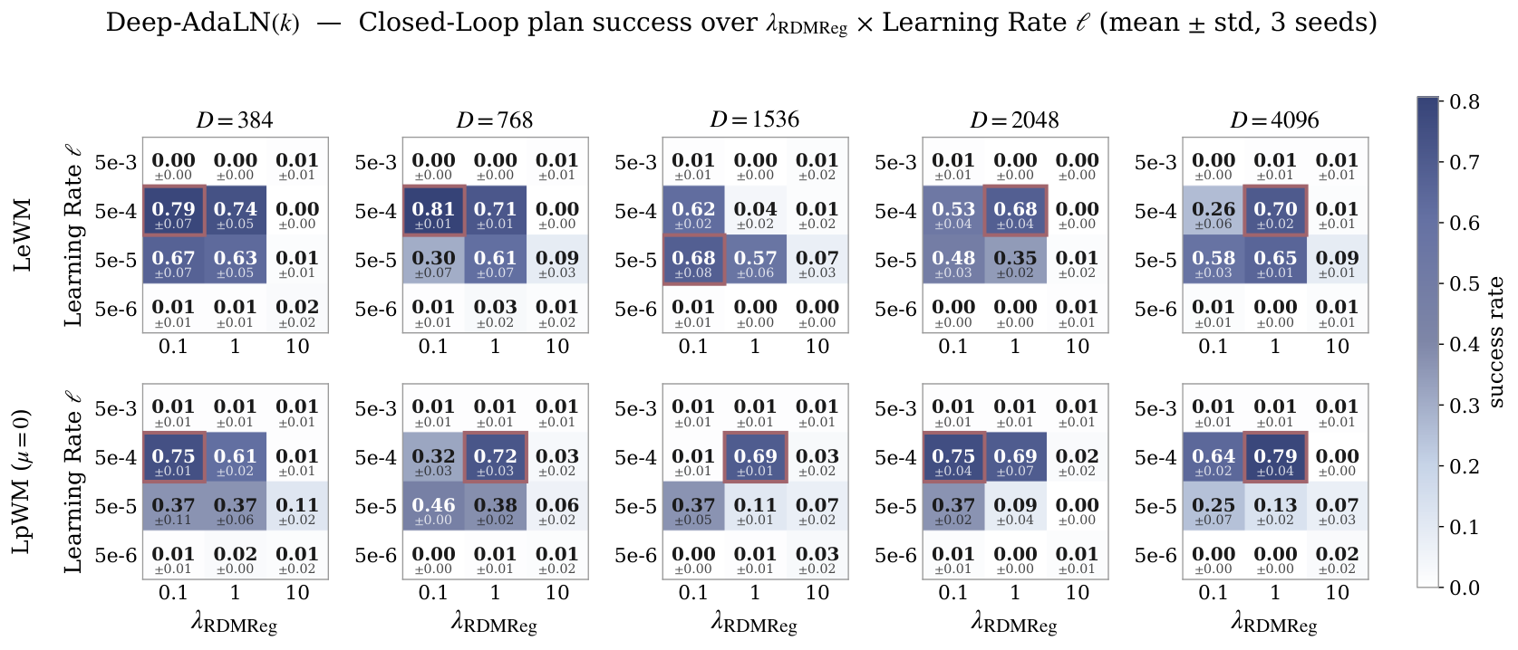
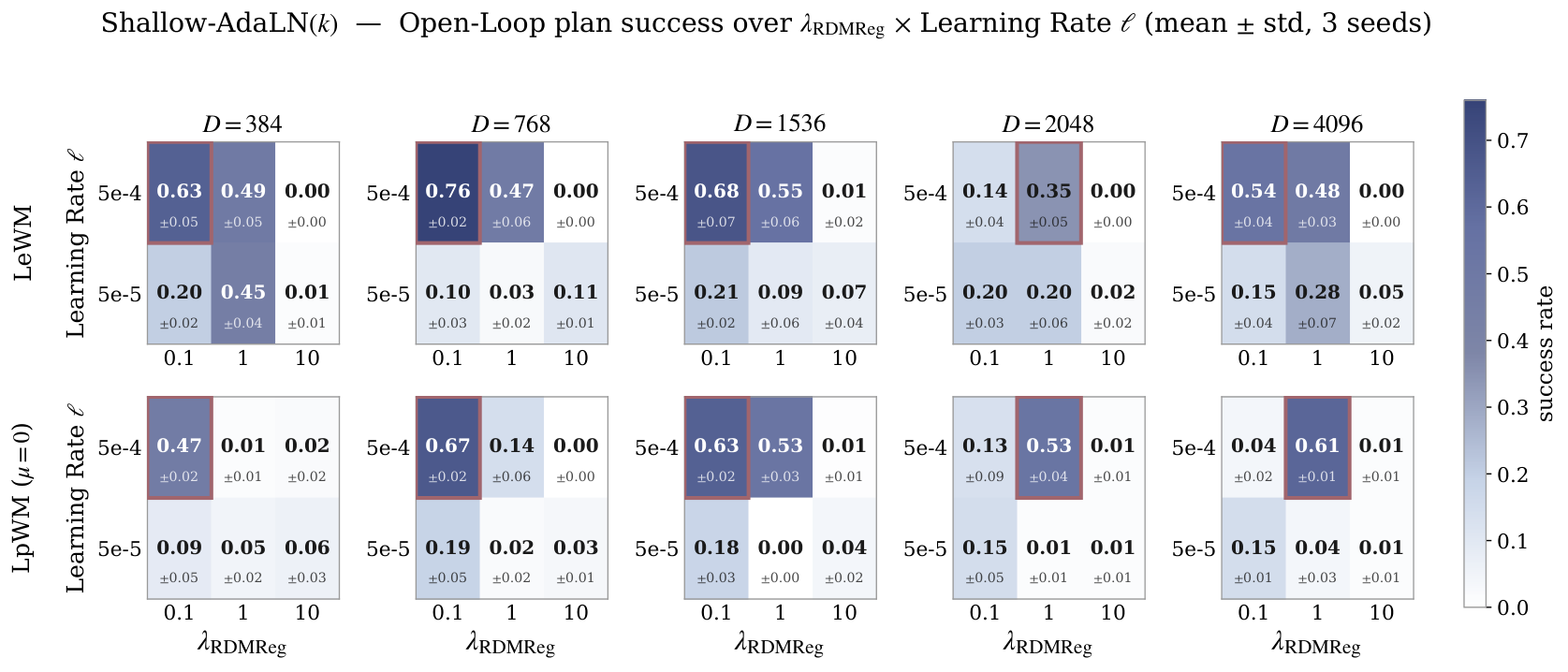
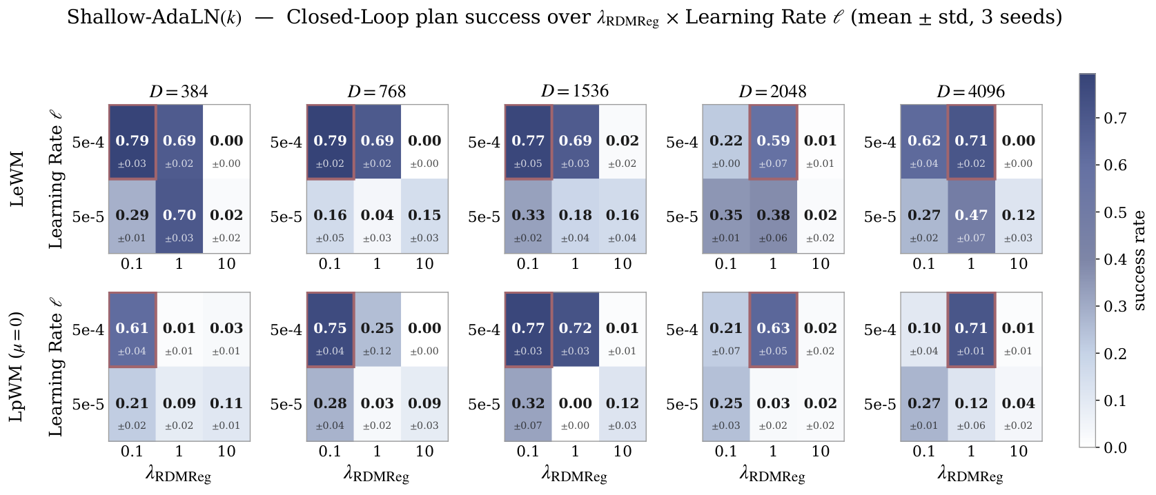
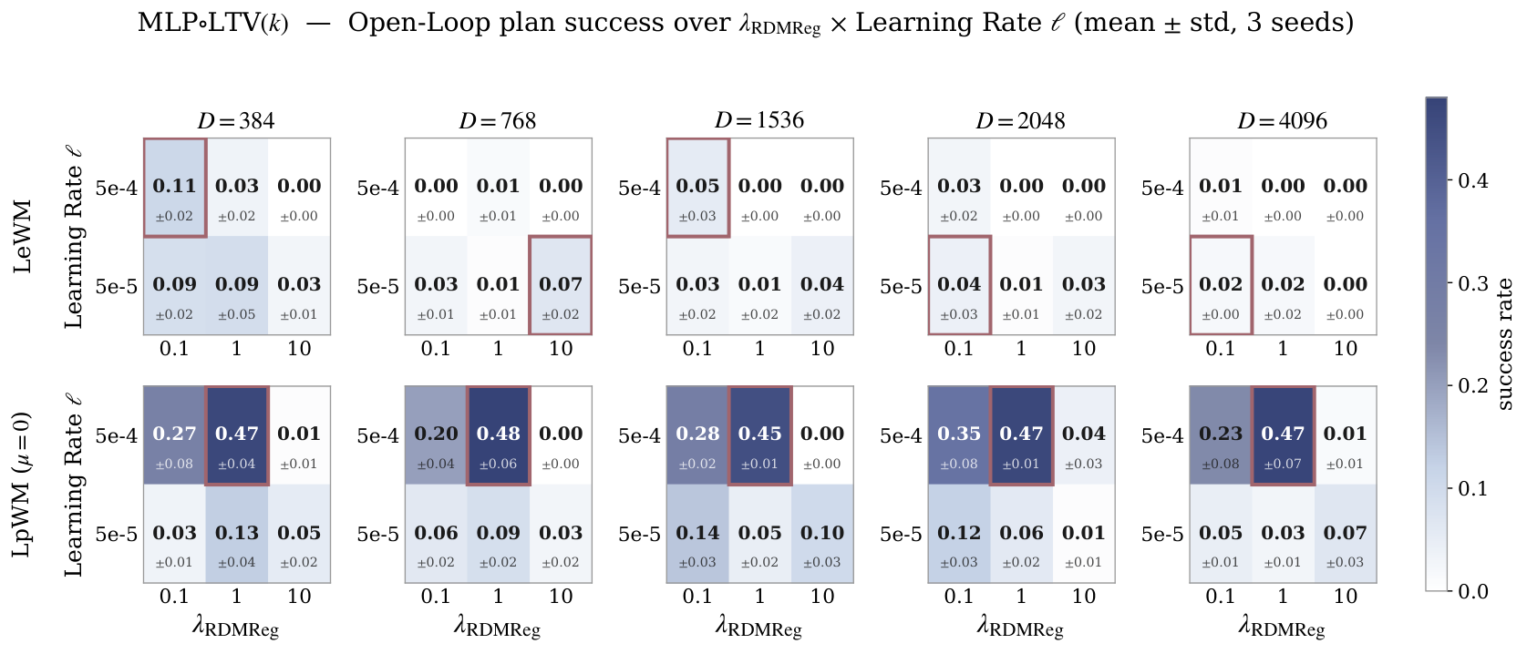
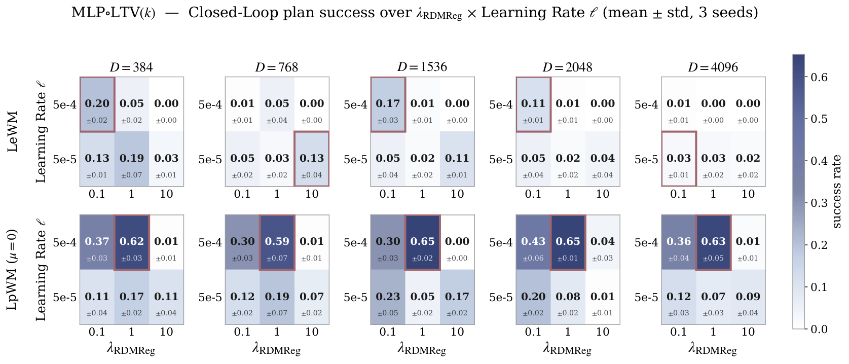
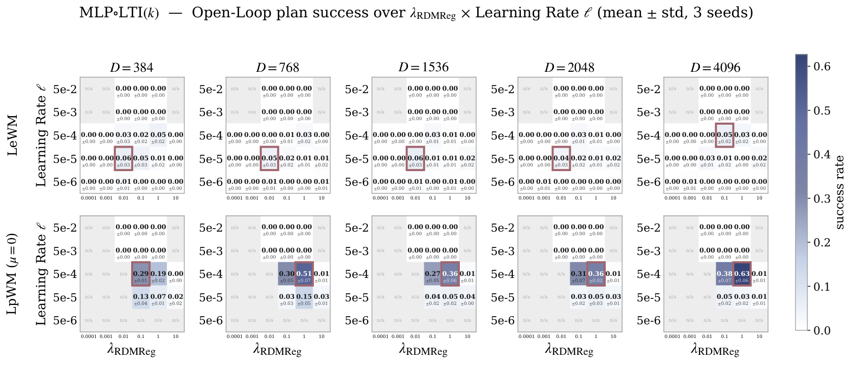
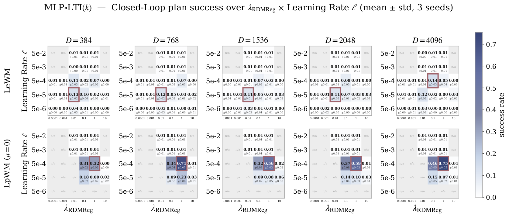
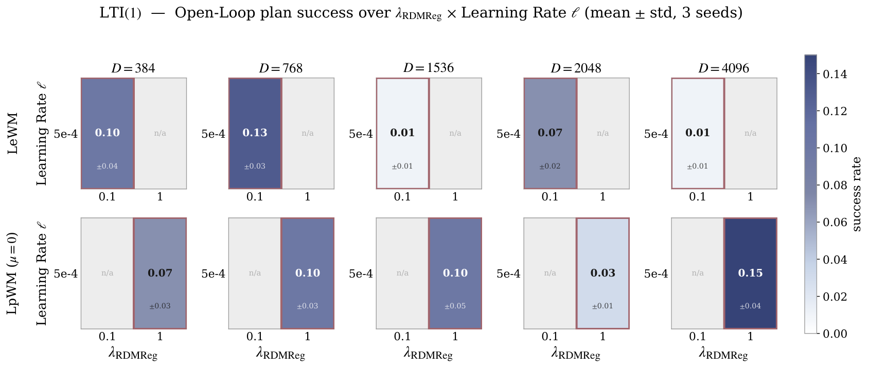
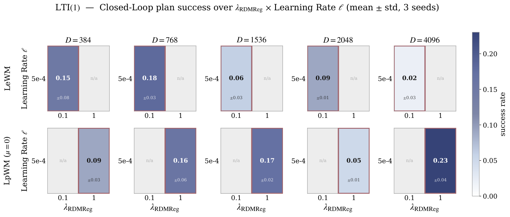
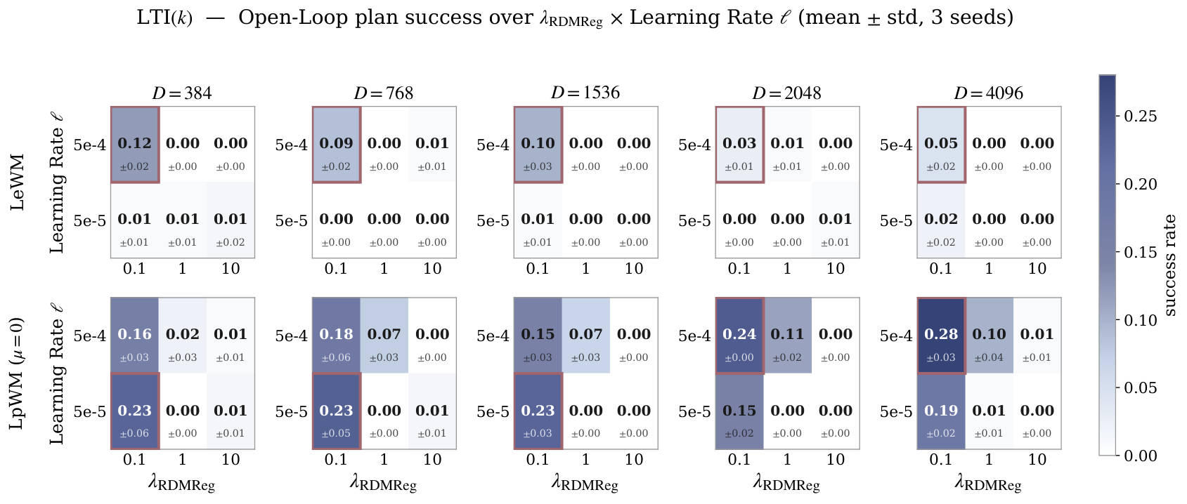
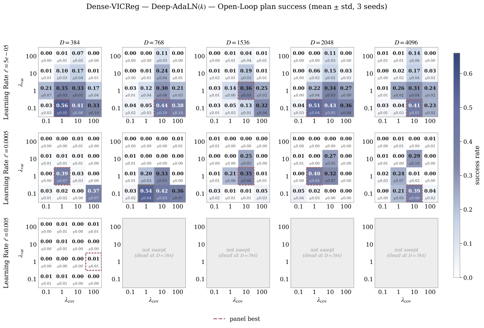
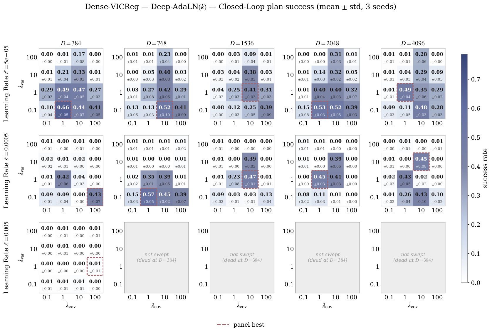
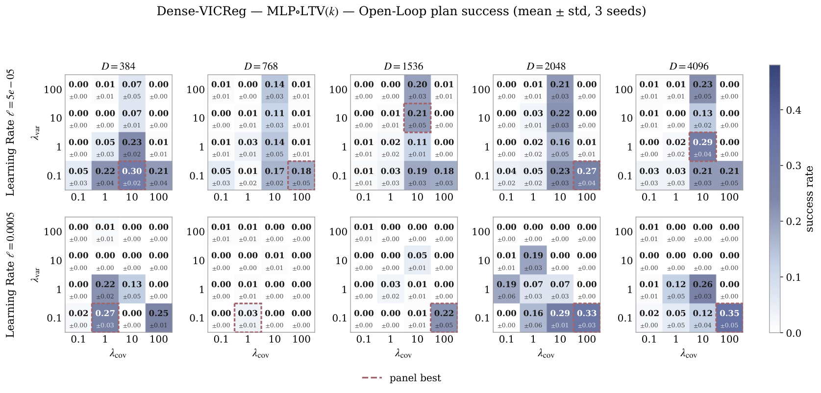
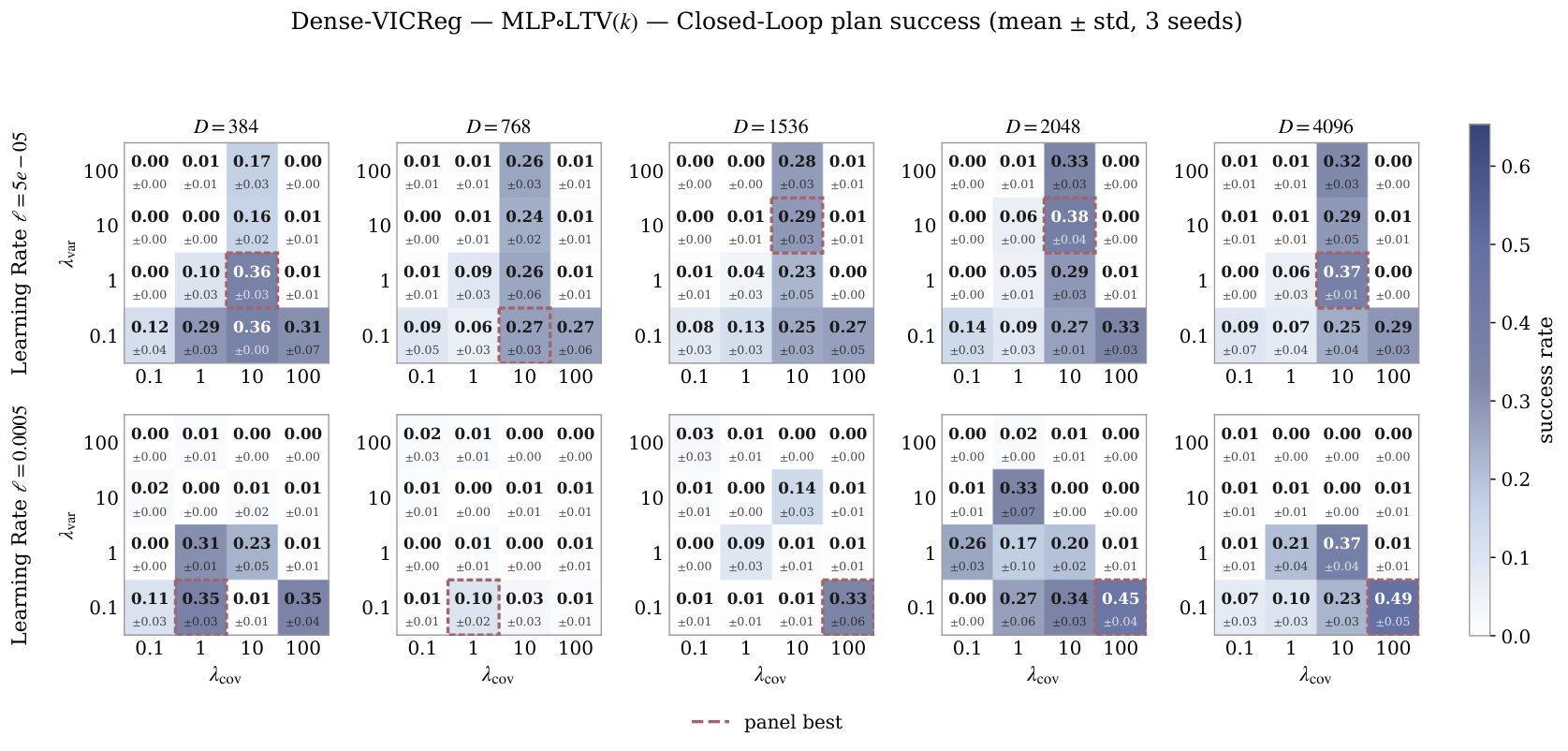
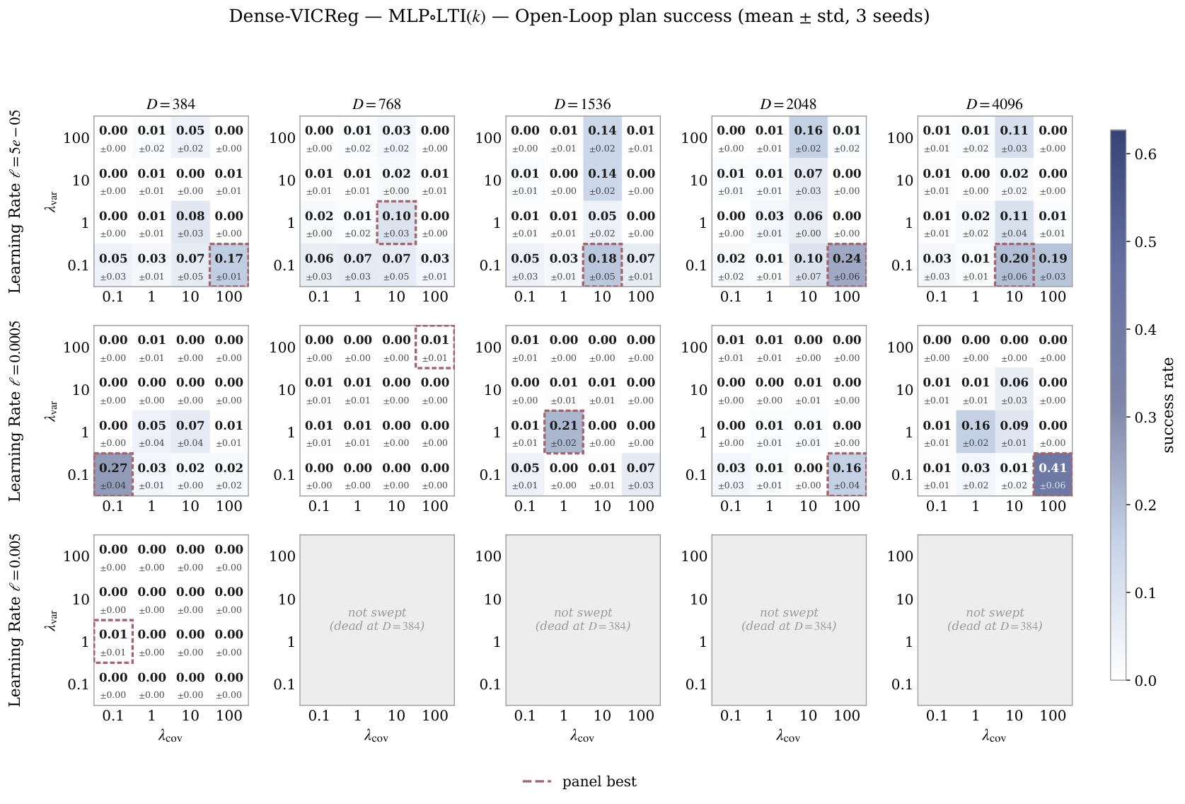
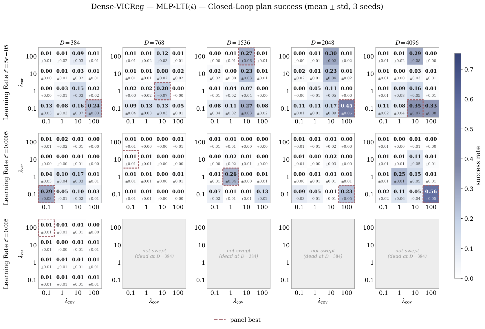
The sweeps vary feature width, regularization weight and learning rate for both sparse and dense targets. Both use sliced-Wasserstein matching here, rather than using the published Gaussian baseline’s different distribution test. Training uses one seed; planning is averaged over three seeds. Later grids omit settings found unsuccessful earlier, so the sweep coverage is not identical for every predictor.
The extra sweeps replace Gaussian distribution matching with VICReg while keeping the world-model setup. “VICReg” names that dense baseline variant in these plots, not a separate general-purpose world-model architecture.
(a)Open-Loop.
(b)Closed-Loop.
Figure 6: Deep-AdaLN Predictor. Hyperparameter Sweeps for the PushT Environment.
(a)Open-Loop.
(b)Closed-Loop.
Figure 7: Shallow-AdaLN Predictor. Hyperparameter Sweeps for the PushT Environment.
(a)Open-Loop.
(b)Closed-Loop.
Figure 8: MLPLTV Predictor. Hyperparameter Sweeps for the PushT Environment.
(a)Open-Loop.
(b)Closed-Loop.
Figure 9: MLPLTI Predictor. Hyperparameter Sweeps for the PushT Environment.
(a)Open-Loop.
(b)Closed-Loop.
Figure 10: LTI Predictor. Hyperparameter Sweeps for the PushT Environment.
(a)Open-Loop.
(b)Closed-Loop.
Figure 11: LTI Predictor. Hyperparameter Sweeps for the PushT Environment.
(a)Open-Loop.
(b)Closed-Loop.
Figure 12: Deep-AdaLN Predictor. Hyperparameter Sweeps for VICReg-based JEPA models in the PushT Environment.
(a)Open-Loop.
(b)Closed-Loop.
Figure 13: MLPLTV Predictor. Hyperparameter Sweeps for VICReg-based JEPA models in the PushT Environment.
(a)Open-Loop.
(b)Closed-Loop.
Figure 14: MLPLTI Predictor. Hyperparameter Sweeps for VICReg-based JEPA models in the PushT Environment.
46 references
Assran et al. (2023)M. Assran, Q. Duval, I. Misra, P. Bojanowski, P. Vincent, M. Rabbat, Y. LeCun, and N. BallasSelf-supervised learning from images with a joint-embedding predictive architecture.
External Links: 2301.08243,
Link
Assran et al. (2025)M. Assran, A. Bardes, D. Fan, Q. Garrido, R. Howes, Mojtaba, Komeili, M. Muckley, A. Rizvi, C. Roberts, K. Sinha, A. Zholus, S. Arnaud, A. Gejji, A. Martin, F. R. Hogan, D. Dugas, P. Bojanowski, V. Khalidov, P. Labatut, F. Massa, M. Szafraniec, K. Krishnakumar, Y. Li, X. Ma, S. Chandar, F. Meier, Y. LeCun, M. Rabbat, and N. BallasV-jepa 2: self-supervised video models enable understanding, prediction and planning.
External Links: 2506.09985,
Link
Balestriero et al. (2023)R. Balestriero, M. Ibrahim, V. Sobal, A. Morcos, S. Shekhar, T. Goldstein, F. Bordes, A. Bardes, G. Mialon, Y. Tian, A. Schwarzschild, A. G. Wilson, J. Geiping, Q. Garrido, P. Fernandez, A. Bar, H. Pirsiavash, Y. LeCun, and M. GoldblumA cookbook of self-supervised learning.
External Links: 2304.12210,
Link
Balestriero and LeCun (2025)R. Balestriero and Y. LeCunLeJEPA: provable and scalable self-supervised learning without the heuristics.
External Links: 2511.08544,
Link
Bardes et al. (2024)A. Bardes, Q. Garrido, J. Ponce, X. Chen, M. Rabbat, Y. LeCun, M. Assran, and N. BallasRevisiting feature prediction for learning visual representations from video.
External Links: 2404.08471,
Link
Bardes et al. (2022)A. Bardes, J. Ponce, and Y. LeCunVICReg: variance-invariance-covariance regularization for self-supervised learning.
External Links: 2105.04906,
Link
Brunton et al. (2016)S. L. Brunton, J. L. Proctor, and J. N. KutzDiscovering governing equations from data by sparse identification of nonlinear dynamical systems.
Proceedings of the national academy of sciences113 (15), pp. 3932–3937.
Chakraborty et al. (2025)D. Chakraborty, Y. LeCun, T. G. J. Rudner, and E. Learned-MillerImproving pre-trained self-supervised embeddings through effective entropy maximization.
External Links: 2411.15931,
Link
Chen et al. (2020)T. Chen, S. Kornblith, M. Norouzi, and G. HintonA simple framework for contrastive learning of visual representations.
External Links: 2002.05709,
Link
Dosovitskiy et al. (2021)A. Dosovitskiy, L. Beyer, A. Kolesnikov, D. Weissenborn, X. Zhai, T. Unterthiner, M. Dehghani, M. Minderer, G. Heigold, S. Gelly, J. Uszkoreit, and N. HoulsbyAn image is worth 16x16 words: transformers for image recognition at scale.
External Links: 2010.11929,
Link
Ermolov et al. (2021)A. Ermolov, A. Siarohin, E. Sangineto, and N. SebeWhitening for self-supervised representation learning.
External Links: 2007.06346,
Link
Goswami et al. (2023)R. G. Goswami, P. Krishnamurthy, and F. KhorramiData-driven deep learning based feedback linearization of systems with unknown dynamics.
In 2023 American Control Conference (ACC),
pp. 66–71.
Grill et al. (2020)J. Grill, F. Strub, F. Altché, C. Tallec, P. H. Richemond, E. Buchatskaya, C. Doersch, B. A. Pires, Z. D. Guo, M. G. Azar, B. Piot, K. Kavukcuoglu, R. Munos, and M. ValkoBootstrap your own latent: a new approach to self-supervised learning.
External Links: 2006.07733,
Link
Hu et al. (2021)E. J. Hu, Y. Shen, P. Wallis, Z. Allen-Zhu, Y. Li, S. Wang, L. Wang, and W. ChenLoRA: low-rank adaptation of large language models.
External Links: 2106.09685,
Link
Hu et al. (2026)J. Hu, Y. Zheng, and T. WangSCALE: state-calibrated latent embeddings for jepa planning in the right geometry.
External Links: 2608.16287,
Link
Jain et al. (2022)A. K. Jain, S. Sujit, S. Joshi, V. Michalski, D. Hafner, and S. Ebrahimi-KahouLearning robust dynamics through variational sparse gating.
External Links: 2210.11698,
Link
Jing et al. (2021)L. Jing, P. Vincent, Y. LeCun, and Y. TianUnderstanding dimensional collapse in contrastive self-supervised learning.
arXiv preprint arXiv:2110.09348.
Korda and Mezić (2018)M. Korda and I. MezićLinear predictors for nonlinear dynamical systems: koopman operator meets model predictive control.
Automatica93, pp. 149–160.
Kuang et al. (2026a)Y. Kuang, Y. Dagade, D. Chakraborty, E. Learned-Miller, R. Balestriero, T. G. J. Rudner, and Y. LeCunRadial-vcreg: more informative representation learning through radial gaussianization.
External Links: 2602.14272,
Link
Kuang et al. (2026b)Y. Kuang, Y. Dagade, T. G. J. Rudner, R. Balestriero, and Y. LeCunRectified lpjepa: joint-embedding predictive architectures with sparse and maximum-entropy representations.
External Links: 2602.01456,
Link
Lesort et al. (2018)T. Lesort, N. Díaz-Rodríguez, J. Goudou, and D. FilliatState representation learning for control: an overview.
Neural Networks108, pp. 379–392.
External Links: ISSN 0893-6080,
Link,
Document
Maes et al. (2026a)L. Maes, Q. L. Lidec, L. Facury, N. Massaudi, A. Chaurasia, F. Capuano, R. Gao, T. Gillin, D. Haramati, D. Scieur, Y. LeCun, and R. BalestrieroStable-worldmodel: a platform for reproducible world modeling research and evaluation.
External Links: 2605.21800,
Link
Maes et al. (2026b)L. Maes, Q. L. Lidec, D. Scieur, Y. LeCun, and R. BalestrieroLeWorldModel: stable end-to-end joint-embedding predictive architecture from pixels.
External Links: 2603.19312,
Link
Pola et al. (2008)G. Pola, A. Girard, and P. TabuadaApproximately bisimilar symbolic models for nonlinear control systems.
Automatica44 (10), pp. 2508–2516.
Proctor et al. (2016)J. L. Proctor, S. L. Brunton, and J. N. KutzDynamic mode decomposition with control.
SIAM Journal on Applied Dynamical Systems15 (1), pp. 142–161.
Rubinstein (1999)R. RubinsteinThe cross-entropy method for combinatorial and continuous optimization.
Methodology and computing in applied probability1 (2), pp. 127–190.
Ružička (1958)M. RužičkaAnwendung mathematisch-statistischer methoden in der geobotanik: synthetische bearbeitung von aufnahmen.
Biológia, Bratislava13, pp. 647–661.
Shang et al. (2026)X. Shang, M. Haseli, J. Cortés, and Y. ZhengOn the existence of koopman linear embeddings for controlled nonlinear systems.
arXiv preprint arXiv:2602.14537.
Sobal et al. (2025)V. Sobal, W. Zhang, K. Cho, R. Balestriero, T. G. J. Rudner, and Y. LeCunLearning from reward-free offline data: a case for planning with latent dynamics models.
External Links: 2502.14819,
Link
Terver et al. (2026)B. Terver, R. Balestriero, M. Dervishi, D. Fan, Q. Garrido, T. Nagarajan, K. Sinha, W. Zhang, M. Rabbat, Y. LeCun, and A. BarA lightweight library for energy-based joint-embedding predictive architectures.
External Links: 2602.03604,
Link
Wang et al. (2026b)Y. Wang, O. Bounou, G. Zhou, R. Balestriero, T. G. J. Rudner, Y. LeCun, and M. RenTemporal straightening for latent planning.
External Links: 2603.12231,
Link
Yang et al. (2022)G. Yang, E. J. Hu, I. Babuschkin, S. Sidor, X. Liu, D. Farhi, N. Ryder, J. Pachocki, W. Chen, and J. GaoTensor programs v: tuning large neural networks via zero-shot hyperparameter transfer.
External Links: 2203.03466,
Link
Yerxa et al. (2023)T. Yerxa, Y. Kuang, E. Simoncelli, and S. ChungLearning efficient coding of natural images with maximum manifold capacity representations.
External Links: 2303.03307,
Link
Zbontar et al. (2021)J. Zbontar, L. Jing, I. Misra, Y. LeCun, and S. DenyBarlow twins: self-supervised learning via redundancy reduction.
External Links: 2103.03230,
Link
Zhang et al. (2026)W. Zhang, B. Terver, A. Zholus, S. Chitnis, H. Sutaria, M. Assran, R. Balestriero, A. Bar, A. Bardes, Y. LeCun, and N. BallasHierarchical planning with latent world models.
External Links: 2604.03208,
Link
Zhou et al. (2025)G. Zhou, H. Pan, Y. LeCun, and L. PintoDINO-wm: world models on pre-trained visual features enable zero-shot planning.
External Links: 2411.04983,
Link