DELE-w0.5: Inferring Action from Future Latent State for Robotic Manipulation

Overview

DELE-w0.5 jointly learns action chunks and a compact future visual state. Its deployed attention mask removes the future-state stream, so inference produces actions without rendering video. Across 640 trials comparing eight methods on four fixed-scene robot tasks, it achieves 62.5% full success and 81.3% ordered-stage progress.

1 Introduction

The paper contrasts VLA policies, which map current context to actions, with world-action models that also predict future observations. It proposes learning action-relevant transitions without reconstructing a dense video trajectory.

Related references: [17], [19], [4], [55], [15], [12], [46], [14], [10].

1.1 Limitation of WAM

Dense future video is expensive and includes many appearance changes unrelated to control. Its large token sequence increases training cost and iterative denoising latency. Compact future-state prediction aims to retain useful transition supervision while reducing this burden.

Related references: [46], [47], [50], [22], [1], [18].

Figure 1: Different Models for Manipulation.

1.2 Our Work

The central change is to jointly model an action chunk and a future endpoint representation instead of every intermediate video frame. The introduction describes action inference from future states; the operational detail in Section 4.4 is that action tokens cannot attend to predicted future tokens, and the latter are omitted at deployment.

2 Related Work

The comparison spans direct VLA policies and approaches using predicted visual futures.

2.1 Vision-Language-Action Models

VLA systems combine pretrained multimodal representations with autoregressive, diffusion, or flow-based action heads. DELE-w0.5 adds future-state prediction as a training objective intended to capture the physical consequences of actions.

Related references: [9], [55], [27], [25], [15], [40], [31], [24], [21], [3], [39], [28], [13], [38], [12], [16], [43], [37].

2.2 World-Action Models

World models provide predictive structure through latent dynamics, image goals, video generation, or trajectory prediction. Recent efficiency methods reduce video-generation cost. DELE-w0.5 uses only a future endpoint during training and removes future visual generation during action inference.

Related references: [11], [30], [10], [5], [41], [8], [52], [54], [35], [51], [7], [2], [23], [46], [53], [45], [1], [18], [29].

3 Preliminary

Inputs are language, multi-view images, and robot state; outputs are continuous action chunks.

3.1 Robotic Manipulation

Each chunk contains 60 future actions. A single arm uses seven action dimensions: relative position, Euler-angle rotation, and gripper state. Bimanual control uses fourteen dimensions.

Equation

\bA_{t}=[\ba_{t+1},\ba_{t+2},\cdots,\ba_{t+H}]

3.2 Language and Vision Tokenization

Qwen3 tokenizes language. DINO-v3 encodes images from a head camera and two wrist cameras into visual features. These features provide spatial information for the policy without reconstructing pixels.

Related references: [44], [32].

Equations 1–2

\displaystyle\hat{\bl}=\mathtt{Text~Encoder}(\bL).

(1)

\displaystyle\hat{\bz}_{t}=\mathtt{Vision~Encoder}(\bO_{t}),

(2)

3.3 Timestep Embedding

A multi-frequency timestep embedding passes through a two-layer MLP. The resulting vector conditions the denoising computation.

Equations 3–5

\displaystyle\tilde{\bt}[j]=\begin{cases}\cos\left(\tau\cdot 10000^{-j/k}\right),&\text{if}~0\leq j<k,\\ \sin\left(\tau\cdot 10000^{-(j-k)/k}\right),&\text{if}~k\leq j<2k,\\ 0,&\text{if}~j=d-1~\&~d\text{ is~an~odd~number}.\end{cases}

(3)

\displaystyle\mathbf{t}=\mathtt{FNN}(\tilde{\bt}),

(4)

\displaystyle\mathbf{t}=\mathtt{Timestep~Embedding}(\tau).

(5)

Refer to caption — Figure 2: Overview of $\mathtt{DELE}$ - $\mathtt{w0.5}$ architecture. The model consists of a condition stream and a noise stream. The condition stream encodes the language instruction $\mathbf{L}$ and current observation $\mathbf{O}_{t}$ , while the noise stream jointly denoises the action chunk $\mathbf{A}_{t}$ and future state $\mathbf{O}_{t+\Delta t}$ . The two streams are coupled through AdaLN-modulated QKV projections and masked attention, enabling unified prediction of the robot action and its corresponding latent future state.

4 Framwork of DELE-w0.5

Two coupled streams process conditioning tokens and noisy prediction targets.

4.1 Condition Stream Block

The condition stream fuses task language with the current scene.

4.1.1 Input and Tokenization

Linear projections map language and visual features into a shared 1,024-dimensional hidden space.

Equation 6

\displaystyle\bl=\mathtt{Projection}(\hat{\bl}),~~\bz_{t}=\mathtt{Projection}(\hat{\bz}_{t}),

(6)

4.1.2 Single-Stream Attention Block

Concatenated language and vision tokens pass through shared self-attention to exchange information across modalities.

Related references: [20], [36].

Equations 7–8

\displaystyle\bZ^{\mathrm{c}}_{t}=\mathtt{cat}(\bl,\bz_{t})=:[\bl,\bz_{t}].

(7)

\displaystyle\hat{\bZ}^{\mathrm{c}}_{t}=\mathtt{Attention}(\bZ^{\mathrm{c}}_{t}),

(8)

4.1.3 AdaLN and Output of Condition Stream

Timestep-conditioned adaptive normalization modulates query, key, and value projections. RMSNorm controls feature scale and QKNorm normalizes queries and keys along each head dimension.

Related references: [48].

Equations 9–13

$\displaystyle\bQ_{\mathrm{c}}=$	$\displaystyle\mathrm{QKNorm}\left\{\bW_{q}(\mathrm{RMSNorm}(\hat{\bZ}^{\mathrm{c}}_{t})\odot\bm{\gamma}_{\mathrm{c}})\right\},$	(9)
$\displaystyle\bK_{\mathrm{c}}=$	$\displaystyle\mathrm{QKNorm}\left\{\bW_{k}(\mathrm{RMSNorm}(\hat{\bZ}^{\mathrm{c}}_{t})\odot\bm{\gamma}_{\mathrm{c}})\right\},$	(10)
$\displaystyle\bV_{\mathrm{c}}=$	$\displaystyle\bW_{v}(\mathrm{RMSNorm}(\hat{\bZ}^{\mathrm{c}}_{t})\odot\bm{\gamma}_{\mathrm{c}}),$	(11)

\displaystyle\bm{\gamma}_{\mathrm{c}}=1+\bW_{\mathrm{Adaln}}\mathbf{t}_{\mathrm{c}}+\mathbf{b}_{\mathrm{Adaln}},

(12)

\mathbf{t}_{\mathrm{c}}\overset{\eqref{timestep-embedding}}{=}\mathtt{Timestep~Embedding}(1);

\displaystyle\mathbf{x}^{\prime}=\mathrm{QKNorm}(\mathbf{x})={\mathbf{x}}/{\|\mathbf{x}\|_{2}};

(13)

4.2 Noise Stream Block

Gaussian noise is interpolated with action targets and future visual latents. The noise stream processes those representations with the same attention machinery, using the sampled flow timestep.

Equations 14–16

\displaystyle\bA^{\tau}_{t}=\tau\bA_{t}+(1-\tau)\bepsilon.

(14)

\displaystyle\hat{\bz}_{t+\Delta t}=

\displaystyle\mathtt{Vision~Encoder}(\bO_{t+\Delta t}),

(15)

\displaystyle\bz^{\tau}_{t+\Delta t}=\tau\hat{\bz}_{t+\Delta t}+(1-\tau)\bepsilon.

(16)

4.3 Flow Matching Objective

Joint attention predicts velocity fields for action chunks and future visual representations. The loss sums action and future-state errors, weighted by a balancing coefficient. Figure 3 specifies which token groups can access one another.

Equations 17–21

\displaystyle\bQ=\mathtt{cat}(\bQ_{\mathrm{c}},\bQ_{\mathrm{n}}),~~~\bK=\mathtt{cat}(\bK_{\mathrm{c}},\bK_{\mathrm{n}}),~~~\bV=\mathtt{cat}(\bV_{\mathrm{c}},\bV_{\mathrm{n}}).

(17)

\displaystyle\hat{\bA}^{\tau}_{t},~\hat{\bz}^{\tau}_{t+\Delta t}=\mathtt{Prejection}(\mathtt{Masked~Attention}(\bQ,\bK,\bV)).

(18)

	$\displaystyle\mathcal{L}_{\mathrm{a}}=$	$\displaystyle\mathbb{E}_{\tau\sim\mathcal{U}_{[0,1]},\bepsilon\sim\calN(\bm{0},\bI)}\left[\left\\|\mathbf{u}_{\mathrm{a}}(\bA^{\tau}_{t},\bz^{\tau}_{t+\Delta t},\bq_{t},\mathbf{l})-(\bA_{t}-\bepsilon)\right\\|_{2}^{2}\right],$		(19)
	$\displaystyle\mathcal{L}_{\mathrm{o}}=$	$\displaystyle\mathbb{E}_{\tau\sim\mathcal{U}_{[0,1]},\bepsilon\sim\calN(\bm{0},\bI)}\left[\left\\|\mathbf{o}_{\mathrm{a}}(\bA^{\tau}_{t},\bz^{\tau}_{t+\Delta t},\bq_{t},\mathbf{l})-(\hat{\bz}_{t+\Delta t}-\bepsilon)\right\\|_{2}^{2}\right].$		(20)

\displaystyle\mathcal{L}=\mathcal{L}_{\mathrm{a}}+\lambda\mathcal{L}_{\mathrm{o}},

(21)

Figure 3: Attention masks for training and inference. Rows are query-token groups and columns are key/value-token groups.

\mathbf{L}

\mathbf{O}_{t}

\mathbf{A}_{t}

, and

\mathbf{O}_{t+\Delta t}

denote language, current observation, action, and predicted future observation, respectively. During training (left),

\mathbf{L}

and

\mathbf{O}_{t}

attend bidirectionally;

\mathbf{A}_{t}

attends to

\{\mathbf{L},\mathbf{O}_{t},\mathbf{A}_{t}\}

; and

\mathbf{O}_{t+\Delta t}

attends to all groups. During inference (right),

\mathbf{O}_{t+\Delta t}

is omitted. Colored and white cells indicate permitted and masked attention, respectively. Multi-view tokens are merged into each observation group, and padded language positions are masked along both dimensions.

4.4 Training and Inference

Language and current-image tokens attend bidirectionally but cannot see targets. Action tokens see the condition and action groups, but not future observations. Future-observation tokens can see all groups. At inference, the future-observation group is removed and the remaining mask stays unchanged. Thus future prediction supplies training supervision without entering the deployed action computation.

5 Experiments

Evaluation separates complete success, intermediate progress, and the stage where execution first fails.

5.1 Experimental Setup

All methods use the same Astribot S1 robot and evaluation conditions.

Robot and tasks.

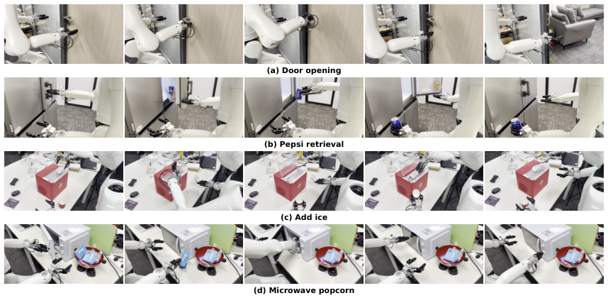
Four tasks test door opening, retrieving a Pepsi can, adding ice to a cup, and heating popcorn in a microwave. A stage counts only after all earlier stages have completed.

Task-suite design.

The suite combines articulated contacts, object retrieval, handoffs, tool use, insertion, and terminal-state checks. Figure 4 illustrates the sequences; Table 1 defines their ordered stages and complete-success conditions.

Table 1: Ordered task stages and complete task conditions. Stage zero denotes no effective progress, and reaching the final stage denotes full task completion.

Task	$K$	Ordered stages	Complete physical state
Door opening	4	Handle contact $\rightarrow$ stable grasp $\rightarrow$ coordinated handle rotation and push $\rightarrow$ sustained opening	Door remains beyond $45^{\circ}$ for at least 3 seconds.
Pepsi retrieval	5	Handle interaction $\rightarrow$ door open $\rightarrow$ can extracted $\rightarrow$ left-hand handoff $\rightarrow$ door closed	Left gripper retains the target can while the refrigerator is closed.
Add ice	6	Scoop pickup $\rightarrow$ lid open $\rightarrow$ cup pickup $\rightarrow$ ice acquired $\rightarrow$ ice poured $\rightarrow$ scene restored	Ice remains in the upright cup and the manipulated scene is restored.
Microwave popcorn	5	Door open $\rightarrow$ package pickup $\rightarrow$ insertion $\rightarrow$ door closed $\rightarrow$ heating started	Popcorn is inside the closed microwave and heating visibly starts.

Baselines and training protocol.

Seven VLA baselines use identical task data for three equivalent fine-tuning epochs under their official configurations. Robot embodiment, instructions, resets, time limits, and scoring are shared. This controls task exposure but does not equalize pretraining histories.

Related references: [34], [6], [12], [42], [49], [33], [26].

Evaluation protocol.

Twenty trials per method and task yield 640 total trials. Each rollout has 180 seconds, receives no physical assistance, and counts as failure if stopped for unsafe execution.

Metrics.

Full success requires the entire physical task. Ordered-stage progress divides the longest completed prefix by the task’s stage count and weights all four tasks equally. Eight raw ice-task annotations are consolidated into six semantic stages.

5.2 Main Results

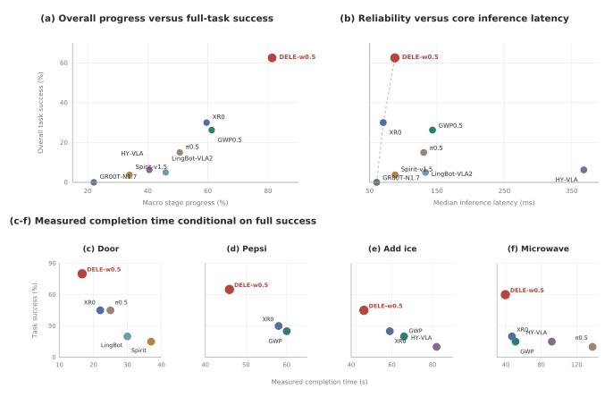
DELE-w0.5 completes 50/80 trials (62.5%) with 81.3% macro progress. Relative to the strongest baseline for each metric, the gains are 32.5 and 20.1 percentage points. Median core-model latency is 87.5 ms on an RTX 4090, excluding networking, image decoding, inverse kinematics, trajectory processing, and robot execution. Completion times in Figure 5 are conditional on successful trials.

Table 2: Real-robot results over twenty trials per task. Each task entry is reported as normalized progress (Prog.) and full-task success (Succ.), in percent. Macro progress weights the four tasks equally; overall success is computed over all 80 trials per method.

	Door		Pepsi		Add ice		Microwave		Macro	Overall
Method	Prog.	Succ.	Prog.	Succ.	Prog.	Succ.	Prog.	Succ.	Prog.	Succ.
$\mathtt{DELE}$ - $\mathtt{w0.5}$ (ours)	95.0	80.0	82.0	65.0	63.3	45.0	85.0	60.0	81.3	62.5
GWP0.5	$80.0$	$45.0$	$60.0$	$25.0$	$50.0$	$20.0$	$55.0$	$15.0$	$61.3$	$26.3$
XR0	$77.5$	$45.0$	$67.0$	$30.0$	$41.7$	$25.0$	$52.0$	$20.0$	$59.5$	$30.0$
$\pi_{0.5}$	$80.0$	$45.0$	$42.0$	$5.0$	$32.5$	$0.0$	$48.0$	$10.0$	$50.6$	$15.0$
LingBot-VLA2	$60.0$	$20.0$	$50.0$	$0.0$	$25.8$	$0.0$	$48.0$	$0.0$	$46.0$	$5.0$
HY-VLA	$57.5$	$0.0$	$35.0$	$0.0$	$37.5$	$10.0$	$32.0$	$15.0$	$40.5$	$6.3$
Spirit-v1.5	$57.5$	$15.0$	$35.0$	$0.0$	$14.2$	$0.0$	$29.0$	$0.0$	$33.9$	$3.8$
GR00T-N1.7	$40.0$	$0.0$	$25.0$	$0.0$	$9.2$	$0.0$	$14.0$	$0.0$	$22.0$	$0.0$

Original figure — Figure 5: Performance and efficiency overview. (a) Macro-average ordered-stage progress versus overall full-task success. (b) Overall success versus median core-model inference latency on an NVIDIA RTX 4090. (c–f) Task-level success versus measured completion-time centers conditional on successful completion. Method abbreviations in the compact task panels correspond to the full names in Table 2 and panels (a)–(b).

5.3 Task-wise and Stage-wise Analysis

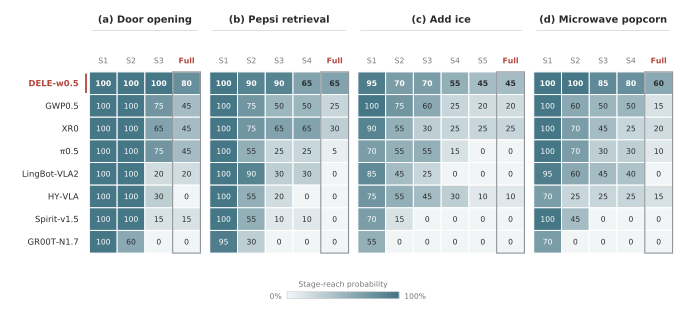
Stage-reach curves show whether a policy converts early progress into complete execution.

Door opening.

Door opening succeeds in 16/20 trials with 95% progress. All twenty reach coordinated handle rotation and pushing; four fail the final sustained-opening requirement.

Pepsi retrieval.

Pepsi retrieval succeeds in 13/20 trials. Eighteen extract the can; later failures cluster around the handoff and refrigerator closure.

Adding ice.

Adding ice succeeds in 9/20 trials. Nineteen pick up the scoop, fourteen reach cup pickup, eleven acquire ice, and nine pour successfully. Tool use and repeated bimanual coordination are the bottlenecks.

Microwave popcorn.

Microwave popcorn succeeds in 12/20 trials with 85% progress. Every trial opens the appliance and picks up the package; sixteen close the door and twelve activate heating.

5.4 Failure Analysis

Failures concentrate at transitions that must preserve earlier progress: rotate-and-push contact, object handoff, precise release, insertion, and final closure. DELE-w0.5 reaches late stages more often but still fails on these transitions.

5.5 Early signs of emergence.

Additional intervention rollouts show the robot reopening a microwave or using the held package to push its door. These are qualitative observations of adaptation, without a quantitative emergence benchmark.

6 Conclusion

Future-state supervision is effective in this four-task, fixed-scene evaluation, while omitting future video reduces deployed computation. The paper does not establish broad scene generalization or quantify the reported intervention behaviors.