Overview
This edition follows the complete 31-page arXiv v2 paper, including all nine appendices. It distinguishes predicting a long action sequence from executing that sequence without feedback. The central result is empirical and data-dependent: longer visual context often makes shorter execution prefixes work better. All 18 numbered figures and their five nested panels, five numbered tables, four original callout diagrams, two displayed equations and 75 references remain.
At a glance
Why do imitation policies often benefit from executing several predicted actions before observing again? The paper argues that a major reason is insufficient history for imitating demonstrations whose actions depend on hidden plans, elapsed time or earlier observations. Experiments on four simulation tasks and two hardware tasks show that increasing context often shifts the best execution horizon toward reactive control. Data-coverage interventions also matter, especially at low data. The conclusion supports testing long-context policies with short execution prefixes, rather than abandoning action-sequence prediction.
1 Introduction
Action chunking combines two choices: how many future actions to predict and how many to execute before replanning. This study holds the future prediction horizon fixed while varying execution. Long open-loop prefixes can preserve a coherent behavior when a short-history imitator cannot infer the demonstrator’s latent state, but they also delay responses to contact or control errors. The proposed remedy is enough observation history to infer that state while continuing frequent replanning. The paper adds a double-encoder architecture and scripted expert variants to study this tradeoff.
2 Related Works
ACT and Diffusion Policy popularized chunked robot control. Prior explanations include reduced compounding error, inference latency, smoothness and mode commitment. Zero-latency simulation isolates effects that cannot be attributed to inference delay alone. Earlier compounding-error analysis remains relevant, particularly with little data; this paper argues that expert history dependence is stronger in its moderate/high-data settings. Adaptive horizons, chunk consistency and reactive refinement heads address related tradeoffs, but do not by themselves identify why a short-context policy fails.
3 Preliminaries
The analysis separates observation history, future prediction length and execution prefix, then distinguishes distribution shift from hidden information in the demonstrator. These mechanisms can coexist.
3.1 Imitation learning and Diffusion Policy
Behavior cloning learns an action-chunk distribution from observation/action demonstrations. The context length counts observed frames; the prediction horizon counts future actions; the execution horizon counts actions used before a fresh policy query. A success–horizon curve varies only the execution prefix for a given trained setup. With a fixed sampling period, the prefix length also determines nominal open-loop duration. Most comparisons predict 15 future actions; short-context baselines observe two frames.
3.2 Compounding Errors in Imitation Learning
Small policy errors can move the robot away from demonstrated states, where further errors accumulate. Longer execution chunks may reduce the number of feedback decisions exposed to that mismatch. DAgger instead labels policy-visited states with expert actions. The paper uses data scale and human-gated DAgger as interventions intended to reduce this source of failure, while acknowledging that they do not perfectly isolate it.
3.3 Non-Markovian experts
An expert is Markovian relative to available observations when current observations suffice to determine its action distribution. A non-Markovian expert also uses earlier states or a latent memory such as a plan or counter. The exposition approximates camera observations as Markovian environment states; real images need not satisfy that assumption. Expert memory and physical partial observability are therefore related but distinct concerns, and “Markovian” must be interpreted relative to the learner’s actual inputs.
4 Expert Markovianity Dominates the Success-Horizon Curve
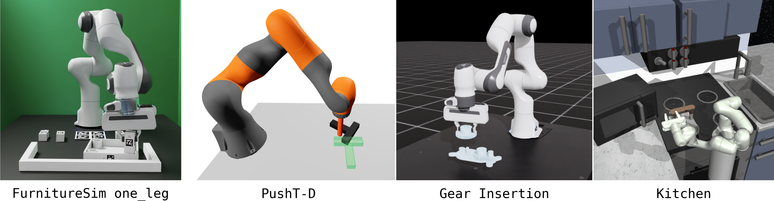
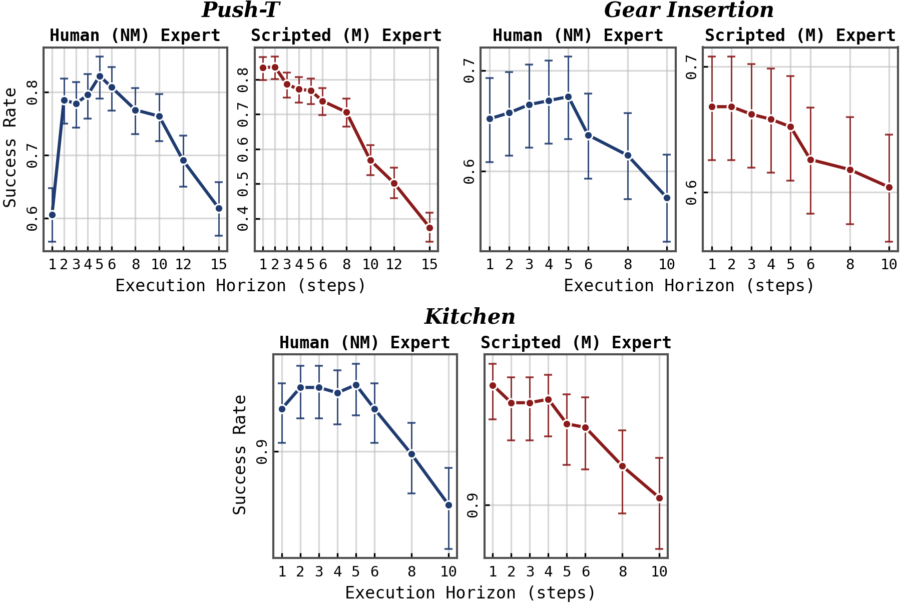
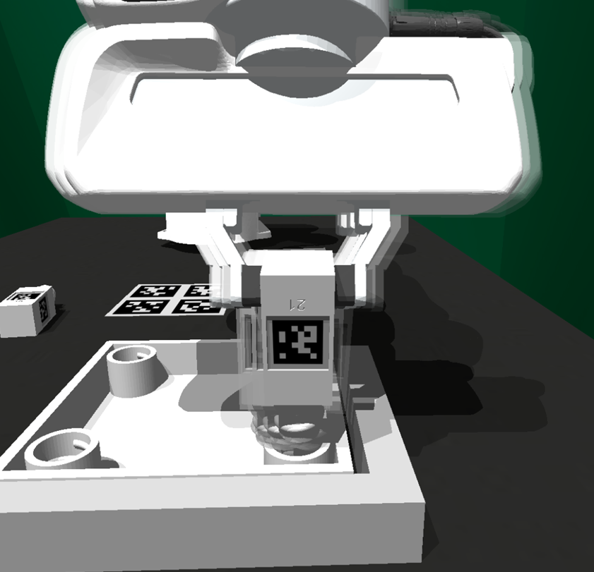
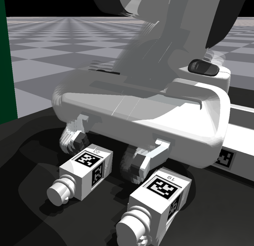
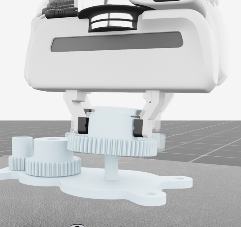
Expert comparisons use image-based Diffusion Policies with two observation frames, 15 future action predictions and execution prefixes from one to 15. Tasks cover furniture assembly, planar pushing, gear insertion and kitchen manipulation. Most datasets contain at least 200 demonstrations. Push-T uses ManiSkill for expert comparisons and Drake for the main context study; their contact models and success conditions differ. Kitchen additionally supplies a subtask-sequence label only for the scripted-expert condition, an important qualification to an otherwise matched comparison.
4.1 Policies Trained on Markovian Expert Demonstrations Exhibit Optimal Execution Horizon T exec ∗ = 1
The experiment asks whether replacing history-dependent demonstrations with observable scripted or learned experts changes which execution horizon performs best. The title’s one-step optimum describes these tested datasets, rather than a universal property of all Markovian-expert imitation.
4.1.1 Experimental Setup
FurnitureSim’s scripted baseline derives its control state from current and previous environment states, so it is observable to a two-frame learner. A second version adds latent waypoint offsets, sticky state transitions lasting up to 16 steps and counted alignment maneuvers lasting up to 30 frames. These introduce deliberately hidden time/plan information. Human teleoperation supplies another history-dependent dataset. Other tasks use deterministic reinforcement-learning or finite-state-machine experts, with details and observation caveats in Appendix A.
4.1.2 Results and Discussion
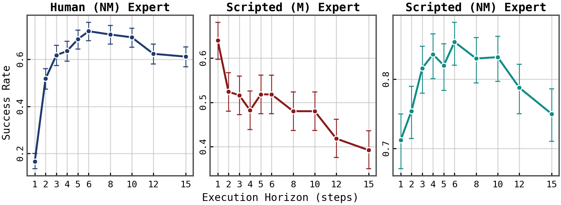
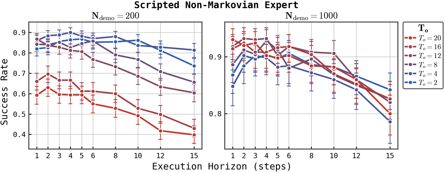
Human demonstrations produce the familiar inverted-U success curves: intermediate execution prefixes work best. Scripted/learned observable experts instead favor the shortest prefixes, with roughly decreasing performance as execution grows. Injecting hidden state into the FurnitureSim expert restores the inverted U. Failure videos show repeated alignment, jitter or switching between locally plausible behaviors without committing to a task transition. These support the hidden-state explanation in the studied settings. Longer open-loop chunks reduce opportunities to change modes, while reactive control helps correct missed insertions and unexpected contact motion.
4.2 Investigating the Role of Compounding Errors
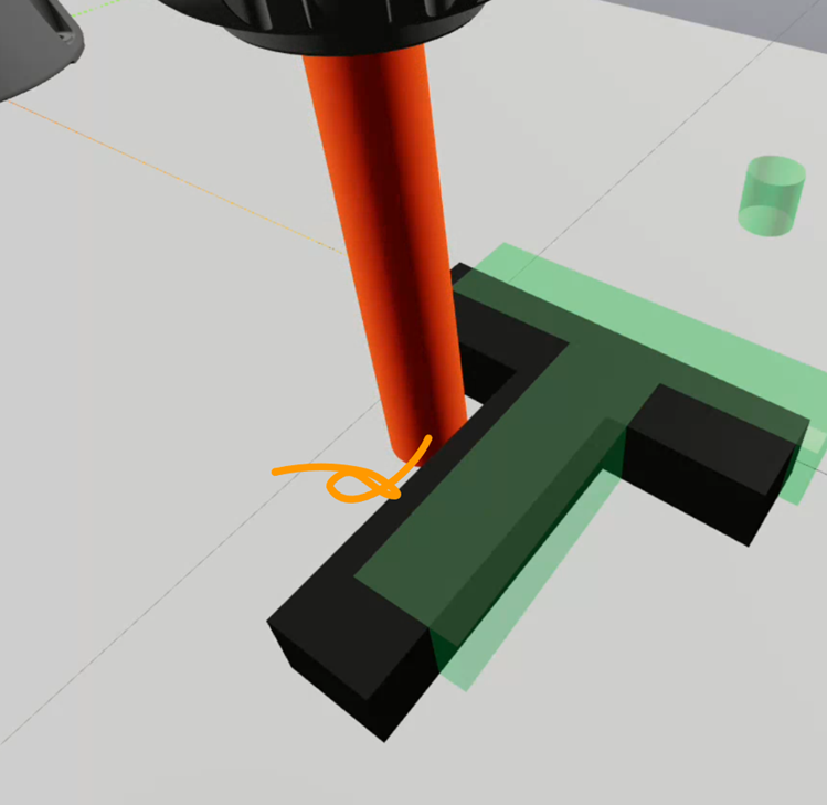
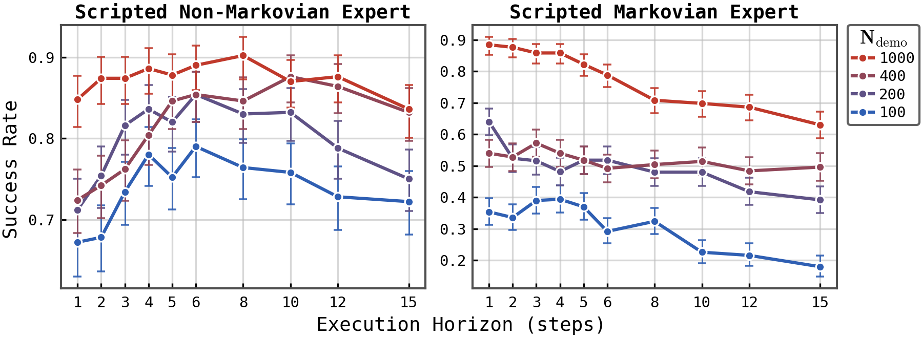
Compounding-error interventions are tested on FurnitureSimOneLeg. With only 100 Markovian demonstrations, the optimum is still a four-action prefix; with 200–1,000, increasing data produces a smaller shift toward reactivity. Thus the findings explicitly retain a low-data case where nontrivial open-loop execution helps despite an observable expert.
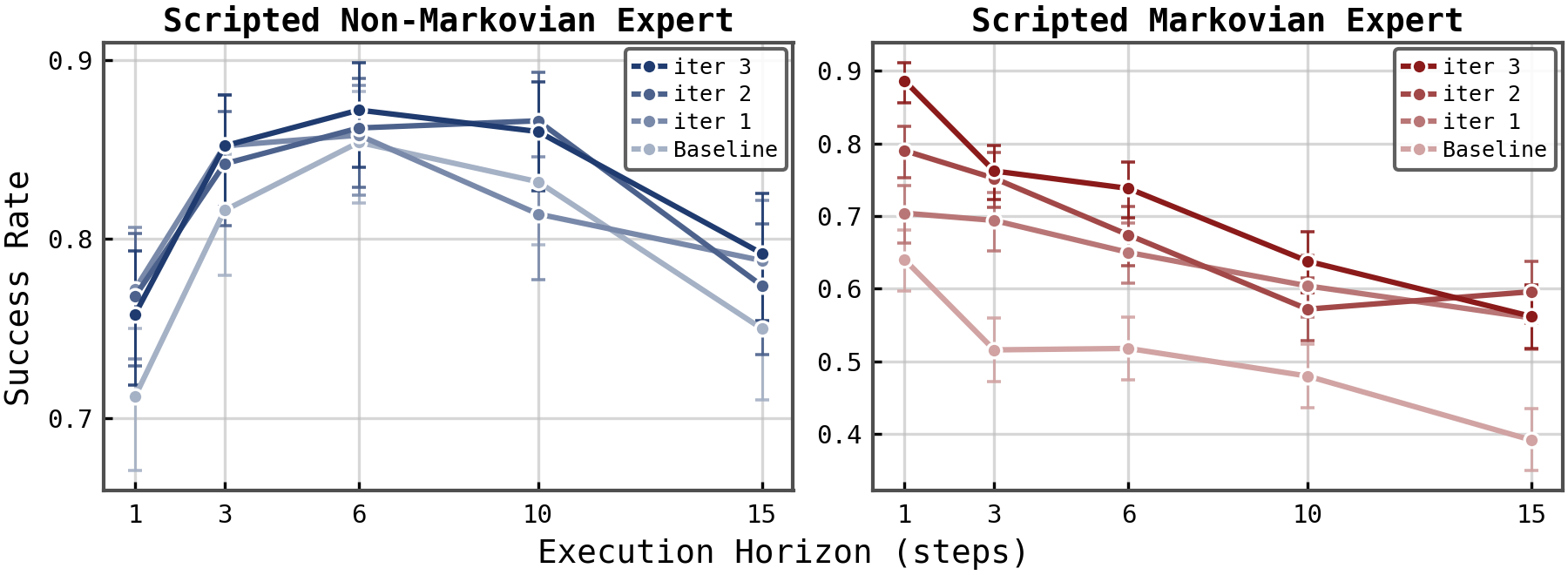
Three human-gated DAgger rounds add 40 correction demonstrations per round for each independently trained horizon branch. The tested prefixes are 1, 3, 6, 10 and 15. Corrections modestly favor shorter prefixes for the Markovian expert but do not noticeably reshape the non-Markovian curve, where corrections retain hidden-state ambiguity. This compares specific interventions on one task; it does not measure or eliminate all compounding error, nor establish the same causal ranking on every benchmark.
5 Long Context Reduces the Need for Long Execution Horizons
The next experiments increase visual history to make more of the expert’s latent state inferable. They evaluate both the relative preference for short execution and absolute task success: an improved horizon curve does not necessarily mean the overall policy improves.
5.1 Methodology
Furniture assembly, gear insertion and hardware tasks use a cross-attention U-Net with separate long-range and short-range image encoders. Both encode the newest two frames; only the long-range encoder sees older frames. During training, the short stream is dropped with probability 0.3, encouraging use of history. PushT-D instead freezes a short-context-pretrained encoder in a FiLM-conditioned U-Net; Kitchen uses a fully tuned FiLM model. The shared qualitative finding spans these choices, while exact gains are not an architecture-independent controlled effect.
5.2 Results and Discussion
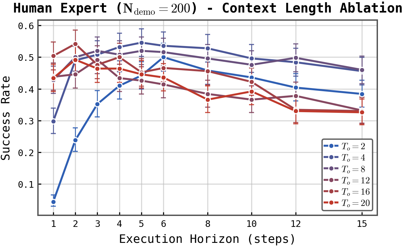
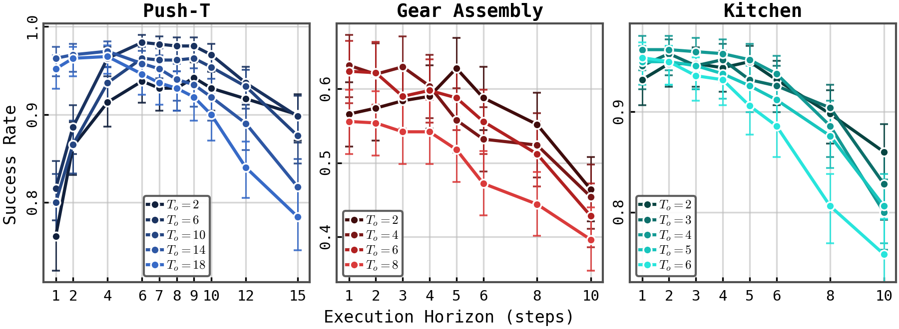
On 200 human furniture demonstrations, moving from two frames to 16–20 shifts the best execution prefix from about six to one or two. Scripted non-Markovian data show stronger absolute results at 1,000 demonstrations: the best long-context/reactive cell reaches 93.2%, compared with 90.6% for the best two-frame policy. Some latent variables remain unobservable even with more history. PushT-D, gear insertion and Kitchen show similar shifts, while Appendix F reports an absolute-performance failure case in PushT-M.
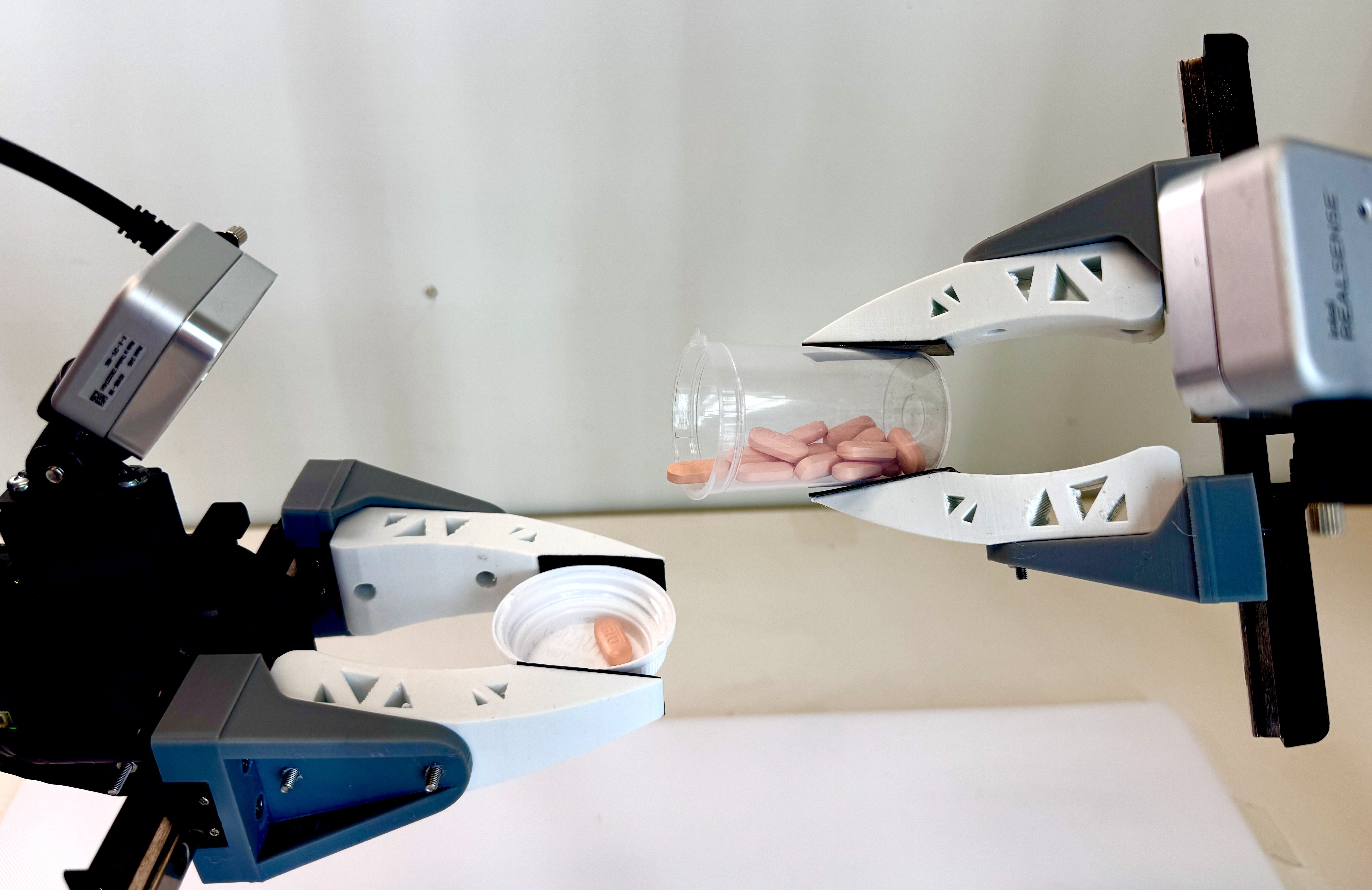
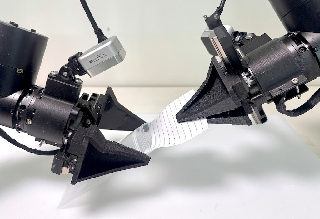
Hardware tests use 516 pill-dispensing and 540 bag-insertion demonstrations. With two-frame context, eight-action prefixes give 75% and 80% success; with eight-frame context, two-action prefixes give 90% and 85% (18/20 and 17/20 trials). These are small independent evaluation sets with broad confidence intervals, not established gains of equal statistical strength. Hardware never tests a one-action prefix. Twelve-frame context worsens the best results in both tasks, showing that more history is not always better at fixed data scale.
| SinglePillDispense | SlipIntoBaggie | |||||
|---|---|---|---|---|---|---|
| 50% [29.9, 70.1] | 60% [38.7, 78.1] | 75% [53.1, 88.8] | 60% [38.7, 78.1] | 40% [21.9, 61.3] | 80% [58.4, 91.9] | |
| 90% [69.9, 97.2] | 80% [58.4, 91.9] | 60% [38.7, 78.1] | 85% [64.0, 94.8] | 70% [48.1, 85.5] | 55% [34.2, 74.2] | |
| 75% [53.1, 88.8] | 70% [48.1, 85.5] | 60% [38.7, 78.1] | 75% [53.1, 88.8] | 65% [43.3, 81.9] | 65% [43.3, 81.9] | |
6 Discussion and Conclusion
The practical implication is to tune context and execution together, with adequate data and checkpoint selection, rather than assume long open-loop execution is essential. The evidence concerns these tasks and policy families; visual memory must support local contact control as well as semantic task recall. Limitations include imperfect observability, task/architecture differences, limited hardware trials and training-selection uncertainty. Long-context inputs increase sample complexity, and their benefits may saturate or reverse.
Acknowledgments
The authors acknowledge research and teleoperation advice, Mundane Systems hardware support, funding from Amazon, the National Science Foundation and Toyota Research Institute, and MIT computing resources.
Appendix A Experimental Setup
The appendix documents task definitions, expert construction, action spaces and hardware evaluation. These details explain which observations make an expert observable and why results across task variants are not interchangeable.
A.1 Benchmark Simulation Task Details
FurnitureSimOneLeg uses low-randomization furniture poses, two cameras and 200 demonstrations per expert. PushT-M uses 300 per expert; the 160-demo PushT-D context study adds a return-to-start success condition and different contact physics. GearInsertion uses three cameras; its “human” data combine 100 teleoperated and 100 MimicGen-generated demonstrations, compared with 200 scripted successes. Kitchen uses 581 human and 581 scripted demonstrations, with any four of seven subtasks required. Tables 2–3 retain each proprioceptive/action space and the action frequencies: 10 Hz furniture/pushing, 30 Hz gear insertion and 12.5 Hz Kitchen.
| Task | Proprioceptive State | Action Space |
|---|---|---|
| FurnitureSimOneLeg | 16D: end-effector pose, velocity, and gripper width | 10D: delta end-effector command (3D translation, 6D rotation, 1D gripper) |
| Push-T | 3D: planar end-effector position and orientation | 2D: delta end-effector position in the XY plane |
| GearInsertion | 9D: 3D end-effector position, 4D orientation quaternion, 2D gripper state | 7D: delta end-effector pose and gripper command |
| Kitchen | 9D: seven arm-joint positions and two gripper-finger positions | 9D: velocity commands for the seven arm joints and two gripper joints |
A.2 Markovian Experts for Push-T , GearInsertion , and Kitchen
PushT-M’s observable expert is a deterministic evaluation of a PPO-trained Gaussian policy. Gear insertion uses a state-based controller with small executed/recorded action noise to broaden supervision. Kitchen samples a four-subtask sequence and exposes it to both the scripted expert and its learner; human-data policies do not receive that label. Scripted observations also receive noise to match the human collection setup. Only successful expert episodes are retained. Success conditioning can itself induce history dependence; the authors expect the effect to be small because expert success exceeds 90%, but do not prove it absent.
A.3 Hardware Experiment Details
Two bimanual tasks test precise feedback under real sensing and inference delay. Their timing, success rules and checkpoint-selection protocol are specified below.
SinglePillDispense .
Starting with bottle and cap already held, the robot must dispense exactly one pill into the cap within 30 seconds; zero or multiple pills fail. The timeout excludes prolonged incoherent shaking that eventually succeeds by chance. Pills weigh approximately 0.6 g; the bottle holds up to 24 and measures 1.7 inches in diameter by 2.8 inches long.
SlipIntoBaggie .
The robot must pick up a bag and paper slip and fully insert the uncreased slip within two minutes. Creasing terminates the attempt as failure. The slip is approximately 83.7×73.8 mm, with ±2 mm variation, and the bag is 127×76.2 mm, making alignment and deformation relevant.
Hardware and control implementation.
Two ARX-5 arms use wrist D405 cameras and an overhead D435. The policy predicts delta end-effector actions at 10 Hz; a 125 Hz interpolator feeds inverse kinematics and joint-position PD control. Observation embeddings are cached. To handle inference delay, execution interpolates from the preceding chunk’s final action to the new chunk’s action 180 ms ahead, an empirically tuned splice. Thus the hardware result includes latency management; a two-action prefix nominally spans 0.2 seconds at the policy action rate.
Evaluation procedure.
Training saves the five checkpoints with lowest validation DDIM mean squared error. Preliminary hardware rollouts screen task performance and qualitative stability, then the selected checkpoint receives an independent 20-trial evaluation. This is distinct from the simulation protocol’s per-horizon best-of-five reporting.
Note on lighting variation.
Color jitter was unintentionally omitted. Evaluations were restricted to the same five-hour daily window, while demonstrations span varying illumination. The suggested benefit of stronger lighting augmentation is a hypothesis, not an evaluated result.
Appendix B Training and Evaluation Methods
Training uses conditional diffusion over action sequences, with task-dependent visual encoders. The validation and checkpoint protocol is essential for interpreting both success curves and uncertainty bars.
B.1 Diffusion Policy
The encoder maps observation history into features, and a conditional U-Net learns to predict injected Gaussian noise at each diffusion noise level. Inference starts from a noisy action chunk and denoises it iteratively. The two original displayed equations retain the corruption process and training objective. Execution uses only the selected prefix before obtaining fresh observations.
Equations
B.2 Training and Evaluation Parameters
Simulation uses ResNet-18, usually R3M-initialized; Push-T uses ImageNet initialization with GroupNorm, while hardware uses DINOv3 at one-tenth the policy learning rate. Cameras have separate encoders, sharing weights over time. Tables 4–5 retain batch size 64, peak policy rate 10−4, cosine scheduling, 500 warmup steps, weight decay 10−6, random crops, 128-dimensional projected features, a 69M-parameter U-Net and ten DDIM inference steps.
Validation holds out 5% of demonstrations, or 2% on hardware, so stated dataset counts include the holdout. Simulation saves checkpoints every five epochs, chooses five by validation loss, evaluates each at each horizon for 500 episodes, and reports the highest-performing checkpoint. Timeouts are approximately 120% of the longest demonstration. Wilson intervals describe finite-rollout uncertainty for the reported checkpoint, without training-seed variability or correction for checkpoint/multiple-policy selection. The authors leave formal multiple-comparison testing to future work.
| Parameter | Value |
|---|---|
| Max LR | |
| LR Scheduler | Cosine |
| Weight Decay | |
| Warmup Steps | 500 |
| Batch Size | 64 |
| Image Size Input | |
| Image Size Encoder | |
| Image Augmentations | 95% random crop |
| Encoder Feature Projection Dim | 128 |
| Parameter | Value |
|---|---|
| U-Net Down dims | |
| U-Net Parameters | 69 million |
| DDIM Inference Steps | 10 |
Appendix C Understanding the Benefits of Long Execution Horizons and Long Context
The following diagrams provide an informal mechanism for the observed curves: limited histories can alias distinct expert states, and action commitment or better context can reduce the resulting ambiguity.
C.1 Why Long Execution Horizons Prevent Failure
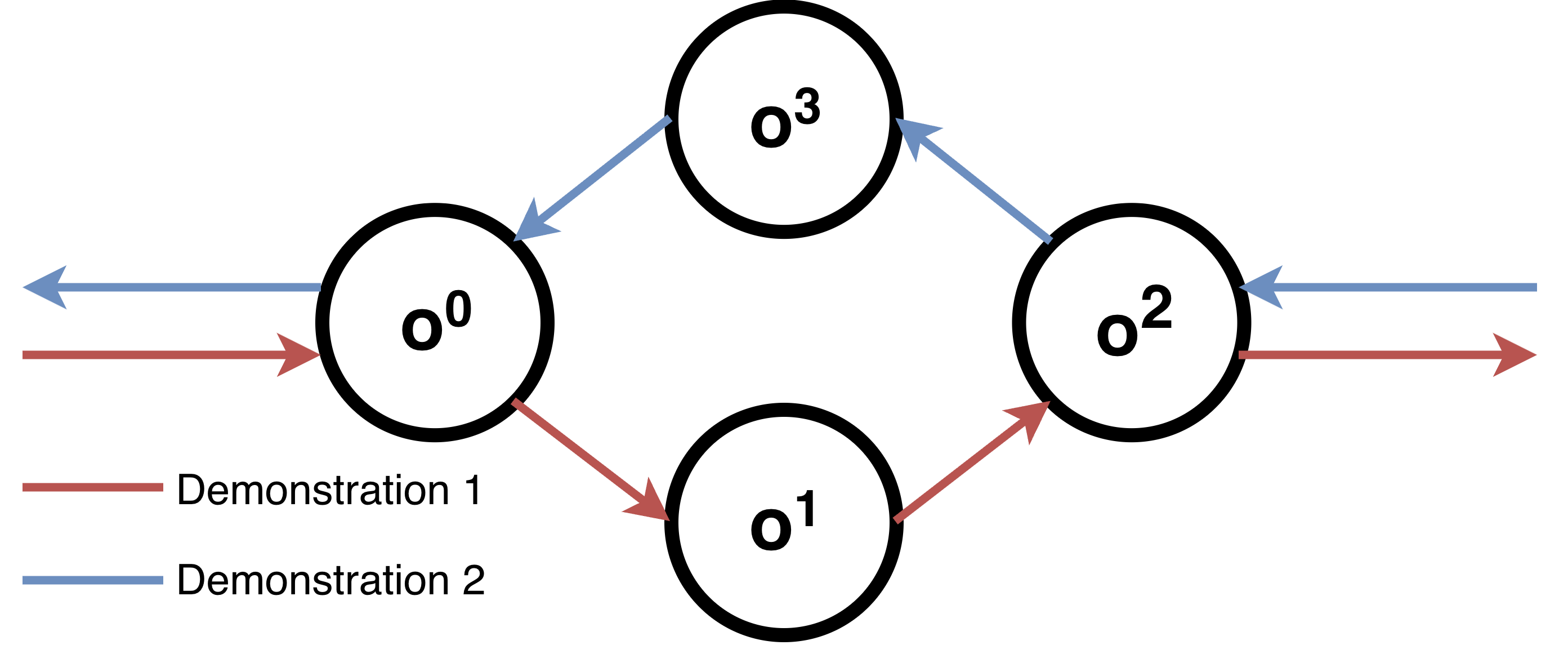
An idle period can look identical at every step to a short-context policy, even when the expert knows when to exit. Across demonstrations, locally valid transitions can also combine into a loop that no individual demonstration contains. Long prefixes can cross these ambiguous regions without resampling a behavior. The appendix’s 1/execution-horizon replanning probability assumes phase is uncorrelated with the aliased state. Its language about immunity to short cycles is an illustrative argument, not a general guarantee for arbitrary learned chunk distributions, dynamics or initial phases; model errors and longer ambiguous regions remain possible.

C.2 Why Long Context Lengths are a Principled Substitute for Long Execution Horizons
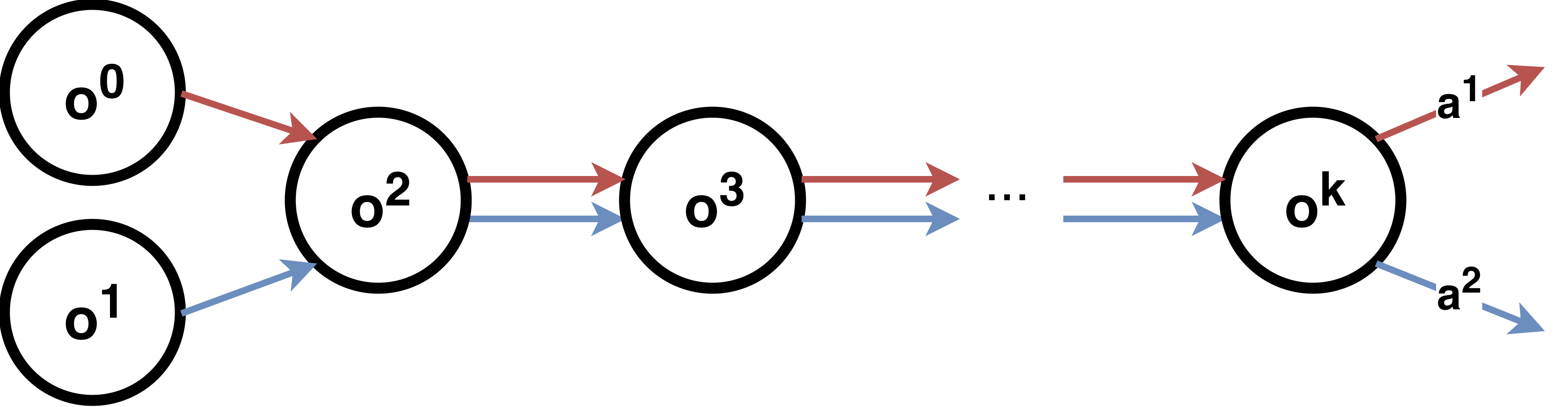
A sufficiently long history can include the earlier observation that distinguishes two otherwise identical present situations, allowing coherent behavior while still replanning frequently. This directly addresses aliasing when the relevant information is observable in history. It cannot recover genuinely unobserved latent choices merely by extending the window.
Appendix D HG-DAgger Implementation Details
Each expert/horizon branch maintains its own correction dataset. In each of three rounds, the best preceding checkpoint is rolled out until 50 failures are collected. One annotator marks the earliest consequential deviation and, for hidden-state experts, the scripted controller state. Simulation resets there; successful expert corrections are collected, discarding episodes after ten failed correction attempts. Forty successful corrections are added when available, followed by 50,000 training steps. Five horizons and two expert types require 1,500 annotated failures. Corrections are never shared across horizons.
Appendix E Exploratory Noise-Injection Experiment
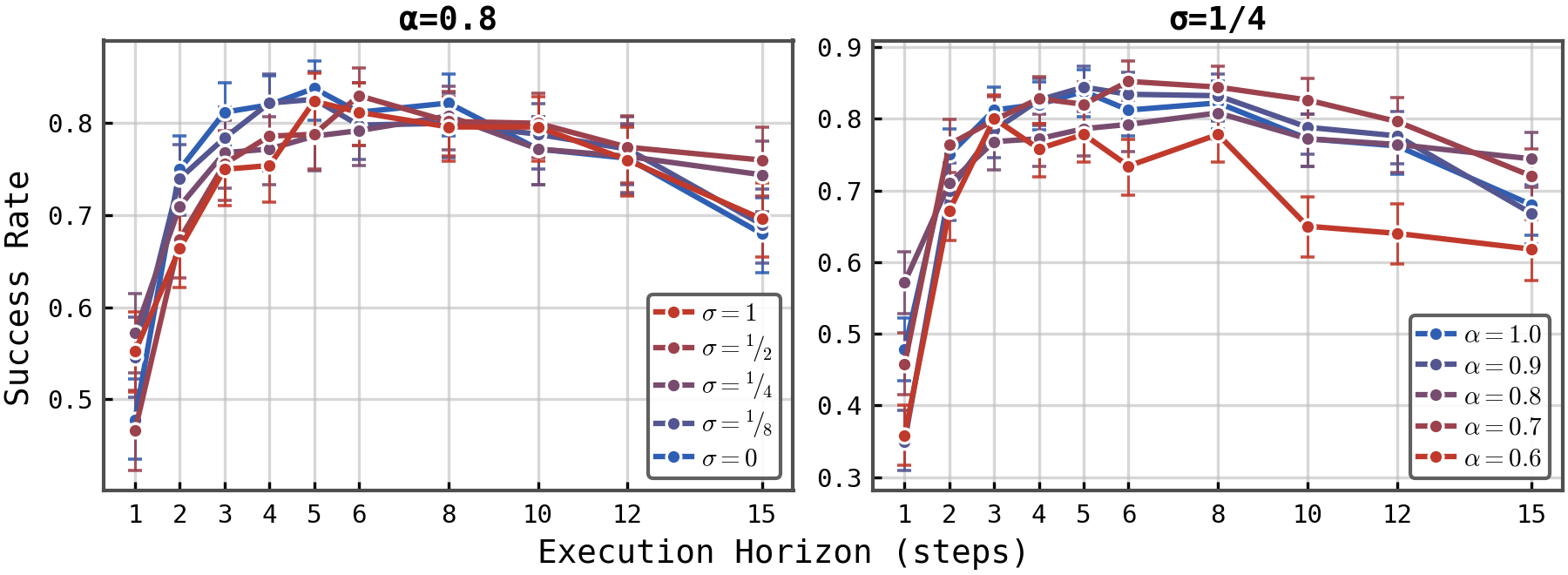
Exploratory data mix clean trajectories with noisy executed actions while recording clean expert labels. The sweep varies clean fraction 0.6–0.9 and state-dependent noise scale 1/16–1. Some settings improve absolute performance at both short and long execution horizons, without a consistent leftward optimum shift. This is not a clean causal test: the non-Markovian expert can add latent-state ambiguity, while later chunk labels are paired with states reached by noisy rather than clean preceding actions. Those biases can favor opposite horizons. The experiment also reduces context to one frame and removes velocity inputs to avoid perturbation/history confounding.
Appendix F Additional Details on Long-Context Training
The appendix specifies the double-encoder implementation and separates its architectural effects from the task-dependent benefits and failures of longer context.
F.1 Double Encoder Method Details
Independent long- and short-range encoders produce a combined sequence of context-length-plus-two tokens. The newest two frames appear in both streams, tagged by temporal and learned range embeddings before cross-attention. With probability 0.3 per training sample, the short stream is replaced by a learned null representation; dropout is disabled at inference. Past-action prediction is also trained: although 15 future actions are fixed, total predicted sequence length grows to 15 plus context length minus one. Context scaling therefore changes the full prediction workload.
F.2 Double Encoder Method Analysis
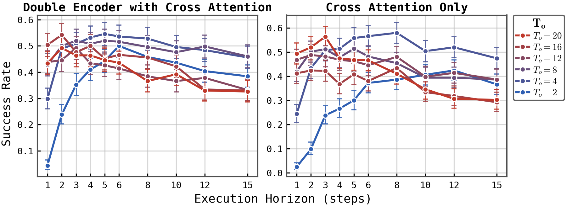
FurnitureSim policies with and without the double encoder show comparable absolute performance and the same qualitative context/horizon trend. The double encoder produces smoother variation across execution horizons. The suggested explanation—redundant immediate-state representations reducing brittleness—is unverified.
F.3 Context Length Ablations for PushT-M
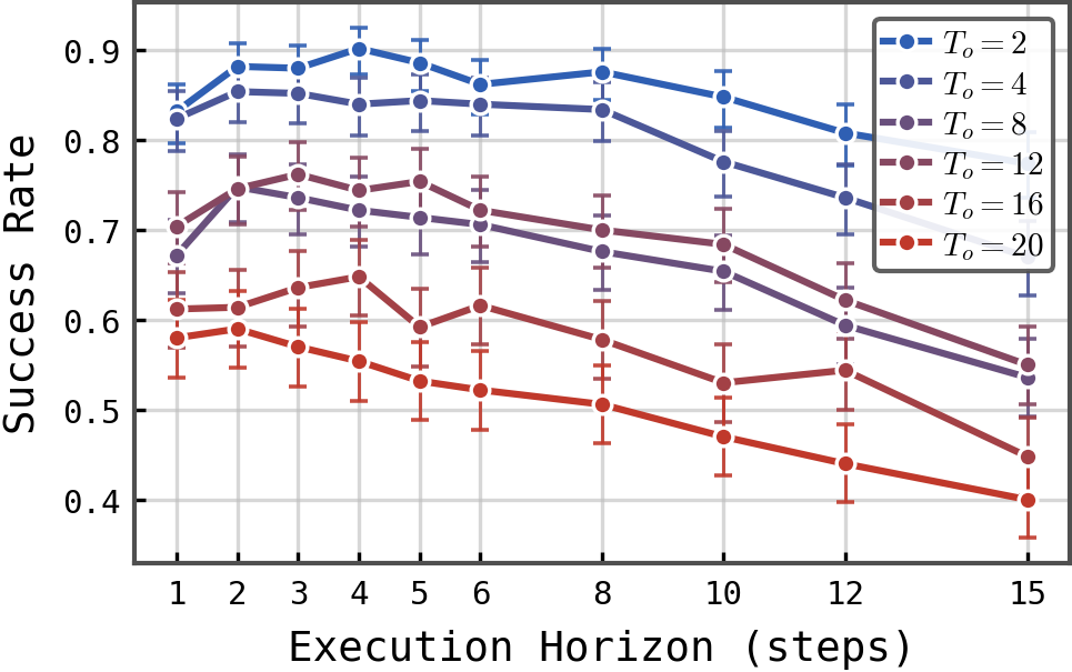
PushT-M is a counterexample to an unconditional “more context improves performance” rule: longer histories favor shorter execution, yet absolute success falls substantially. Sparse visual rendering and causal confusion are proposed explanations, not established causes. With the same two-frame data, the double encoder improves one-step performance relative to the FiLM architecture, but the preferred horizon remains around four or five. Architecture affects the curve as well as context.
Appendix G Additional Discussion: Multimodality and Smooth Execution
The smoothness discussion assumes perfect recovery of the expert conditional distribution. With enough expert-relevant history, sampled trajectories should preserve expert smoothness; with shorter context, recent samples may constrain only local discrete-time smoothness. These idealized arguments do not establish smooth or safe execution for finite-data, imperfect policies, and learning-error analysis is deferred.
Appendix H Additional Discussion: Benefits of Reactivity in Our Experiments
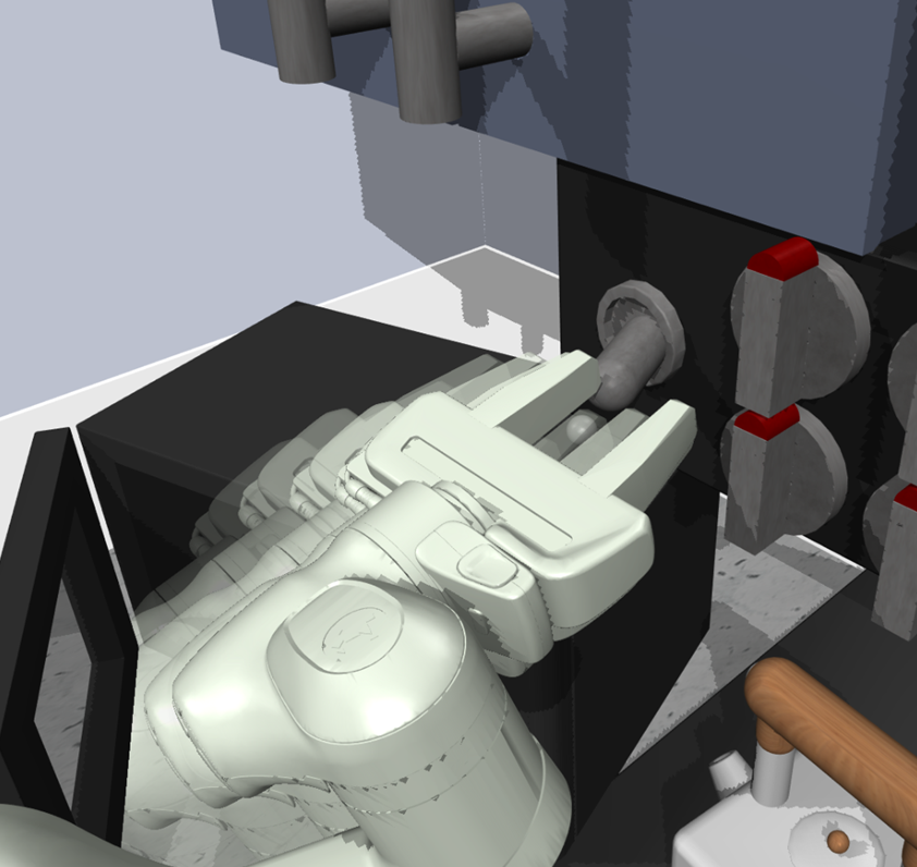
Reactive feedback helps correct table motion during screwing, missed gear insertion, unexpected T-block motion and imprecise kitchen grasps. These observed failures explain why feedback can matter even in nominally static tasks, without requiring external perturbations.
Appendix I Additional Discussion: The Importance of Checkpoint Selection for Long-Context, Reactive Policies
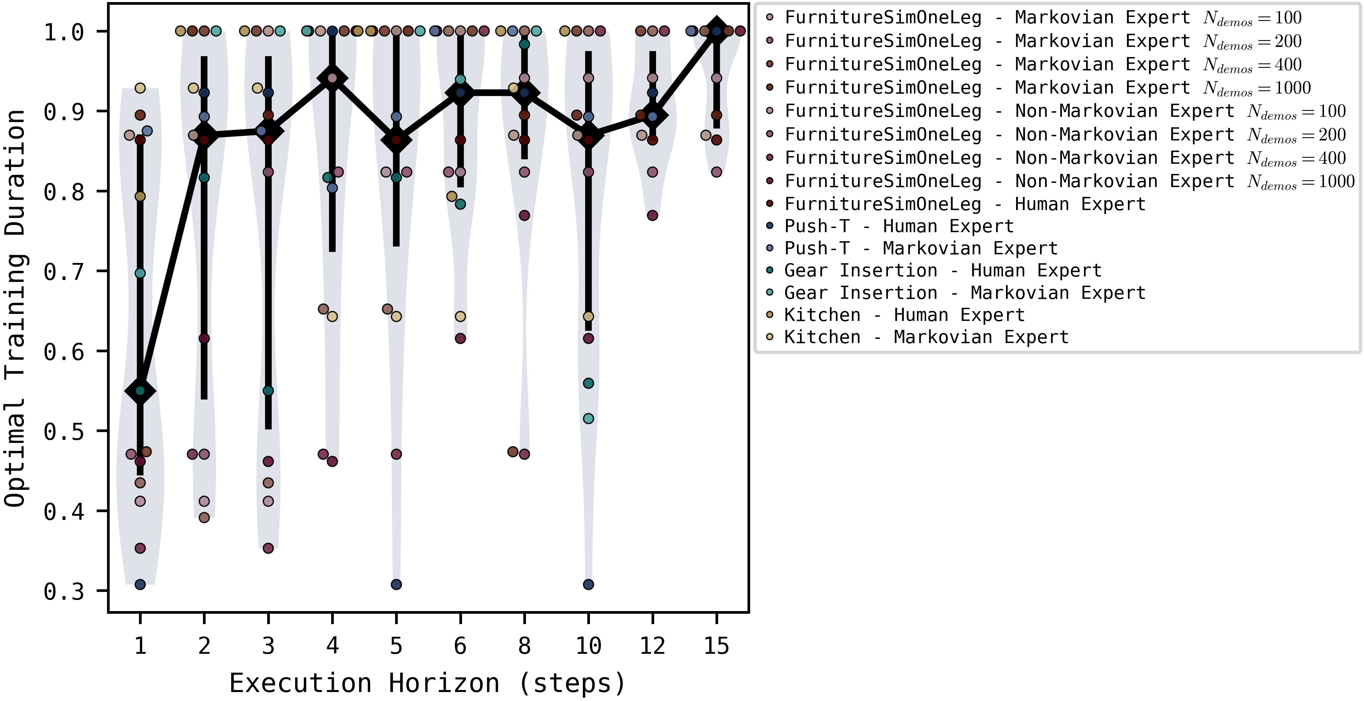
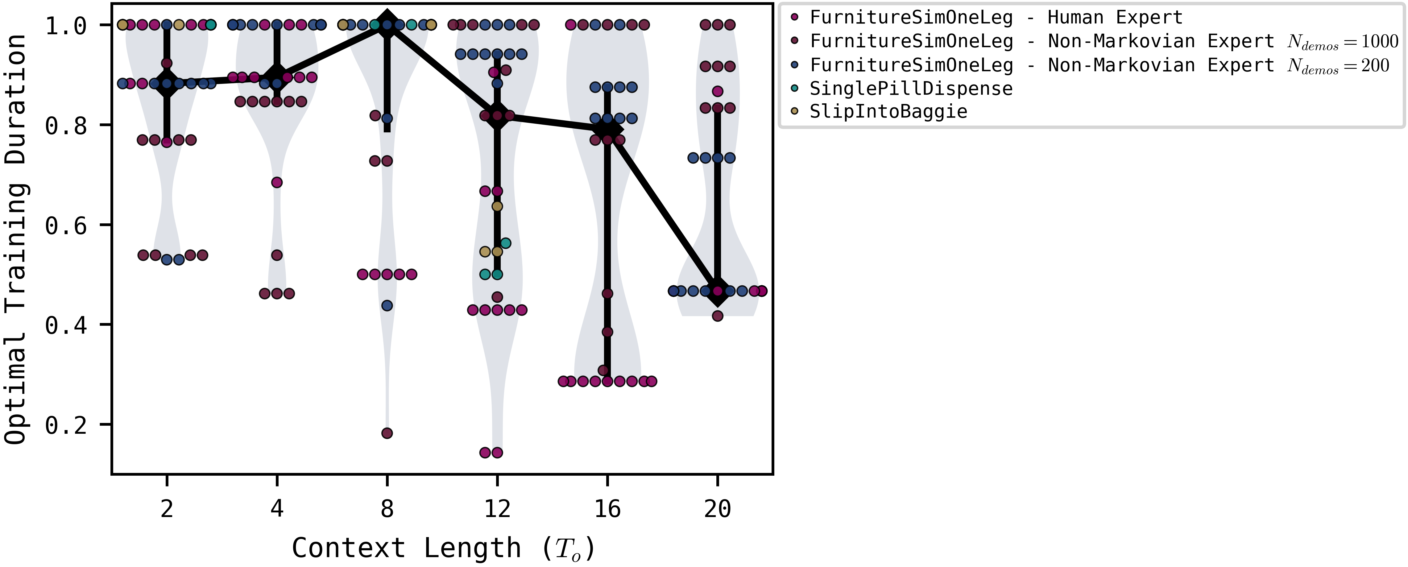
Shorter execution prefixes often favor earlier checkpoints. Longer context also favors earlier checkpoints in furniture assembly and both hardware tasks, but not consistently in Push-T, gear insertion or Kitchen. The plots normalize the best checkpoint epoch by the latest evaluated epoch, and pool heterogeneous settings. Early stopping may reduce distribution-shift sensitivity, but architecture and other variables are confounded. The recommendation is to evaluate checkpoints carefully; stronger claims about large-data reactive policies remain hypotheses.