Overview
The paper combines sampling-based model predictive control, offline-to-online reinforcement learning, and hierarchical whole-body control for state-based locomotion and manipulation.
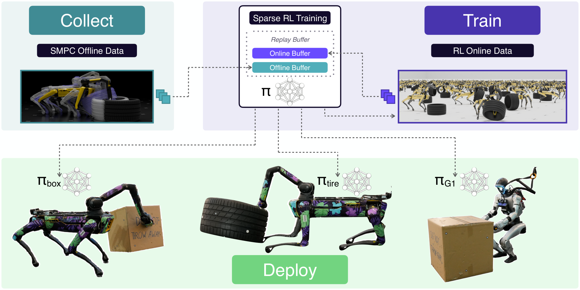
At a glance
A sampling-based model predictive controller generates simulated expert transitions that bootstrap sparse-task-reward reinforcement learning. A high-level learned policy then controls a frozen whole-body stabilizer and transfers to an arm-equipped Spot and a G1 humanoid. Learned policies complete the tested tasks faster than the planner. The method reduces repeated RL reward-shaping cycles, but does not eliminate manual engineering: the planner uses interactively tuned dense costs, the controller and action constraints are designed, and hardware evaluation relies on motion capture.
1 Introduction
Complex locomotion–manipulation tasks make uninformed sparse-reward exploration difficult. The paper moves the initial behavior-design work into a simulator-based planner whose costs can be adjusted while inspecting trajectories, then trains a fast policy from its data and subsequent simulated interaction. The division of labor is useful because teacher behavior need only seed successful exploration, while later reward optimization can improve it. Optimality remains local to the available data and training process.
2 Related Work
The method combines offline-data-assisted online RL [1] with the parallelized FastTD3 [21] implementation. Unlike human teleoperation or motion retargeting, the planner supplies demonstrations for different morphologies through simulation. The contribution is their integration for whole-body tasks with sparse task rewards, rather than a new general solution to planning or reinforcement learning.
3 Learning Loco-Manipulation With SMPC Demonstrations
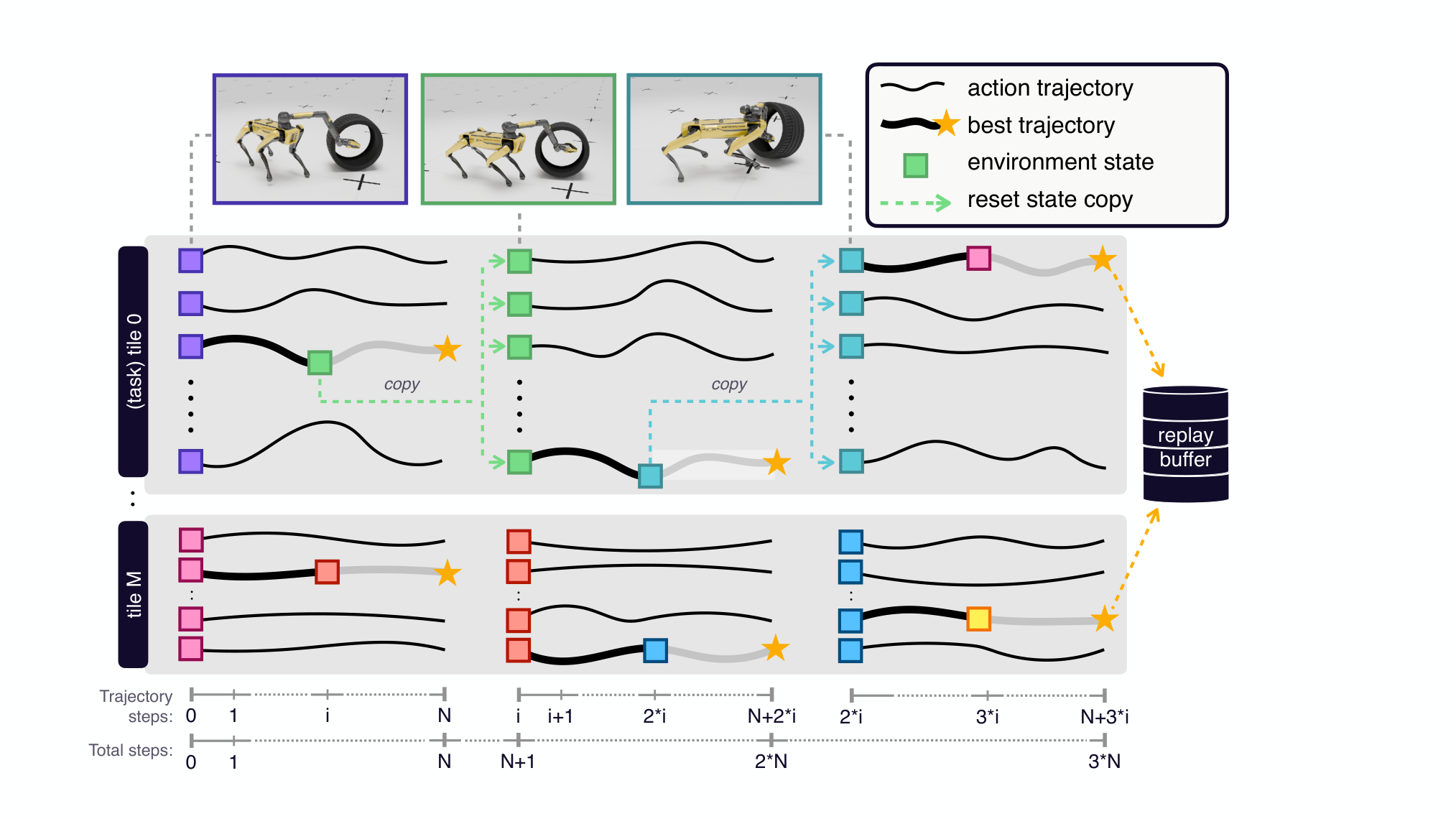
The pipeline shares a hierarchical action interface between data generation and deployment. A simulated planner first supplies successful transitions; a high-level RL policy learns from a mixture of these transitions and its own experience, then gradually relies on online data alone.
3.1 Overview
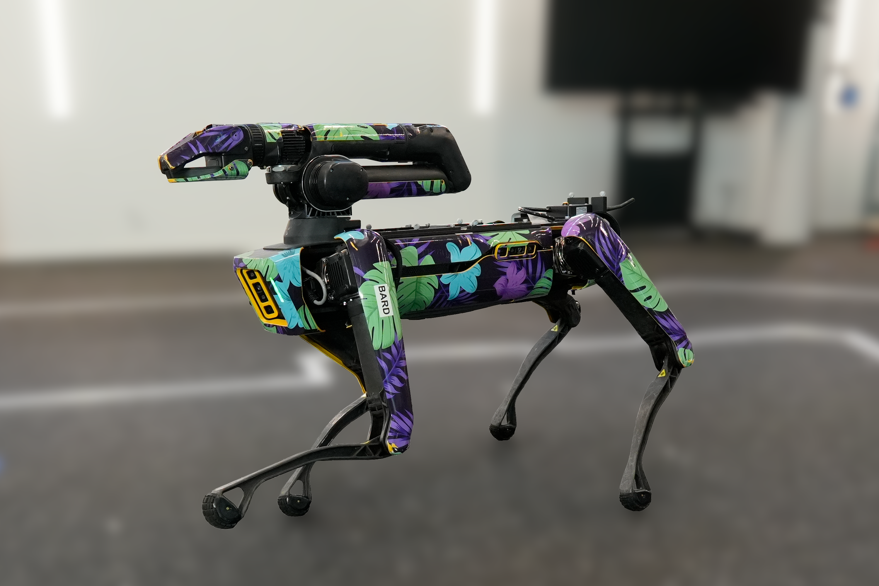
The high-level action changes commanded planar velocity, arm joint targets, and—on G1—torso height and pitch. A pretrained, frozen ReLIC whole-body controller [27] tracks these commands while coordinating the legs for balance. Spot holds torso height and pitch fixed. This decomposition constrains what the task policy can change and delegates dynamic stabilization to a separately trained controller.
3.2 Training Off-Policy RL with Sparse Rewards
The task reward is zero at the goal, minus one per unfinished step, and a terminal crash penalty of −2/(1−γ), with γ=0.99. Thus “sparse” means no dense progress-to-goal shaping; constant time cost and crash penalties still guide the objective. Initially, expert transitions make up half the replay mixture. Once empirical success reaches the chosen threshold, the expert component is removed so learning can improve beyond the teacher distribution.
Action deltas impose speed and acceleration bounds. Critic outputs are bounded using the known return range to reduce overestimation and instability. These constraints and action regularization remain part of the learning system; the claim of tuning-free training should be limited to avoiding repeated dense RL task-reward design.
Equation 1
| (1) |
3.3 Data Collection with Sampling-Based Model Predictive Control
The expert uses the same vectorized simulator with a dense, manually tuned cost. Random trajectory sampling and warm starts are sufficient for the tested tasks. Interactive execution is about half real time on an RTX 5090, allowing rapid qualitative cost adjustment. Tiled sampling scales data collection to roughly one million transitions per hour in the reported setting. The main text’s four-hour summary does not cover every embodiment: the appendix reports more than ten hours for G1 data collection.
4 Experiments
Experiments examine real deployment, completion time, expert dataset size and quality, multimodal demonstrations, and alternatives that directly imitate or reuse the planner’s dense objective. Additional appendix studies test replay mixture, critic bounds, and the expert-data removal threshold.
Real-world deployment on diverse platforms
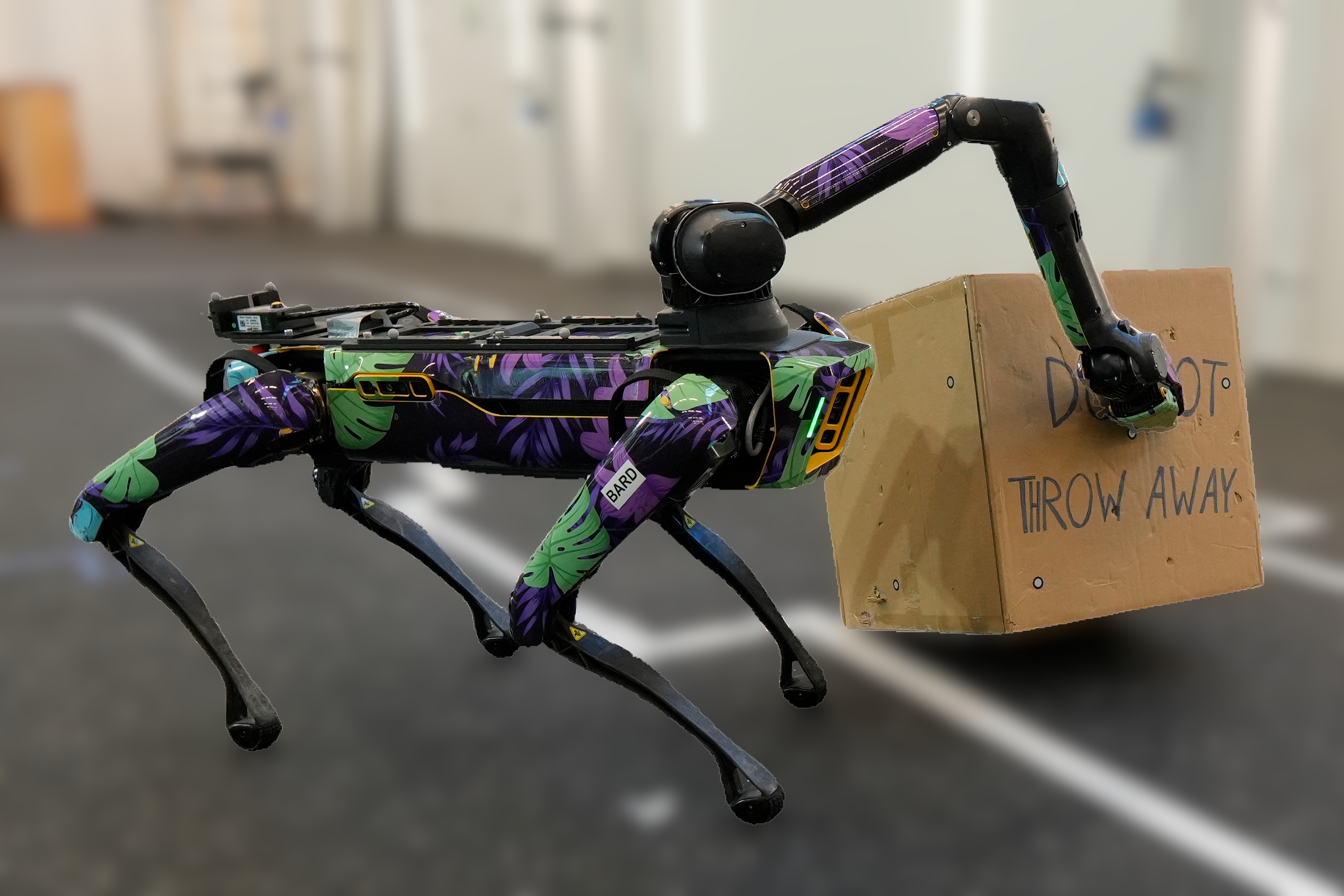
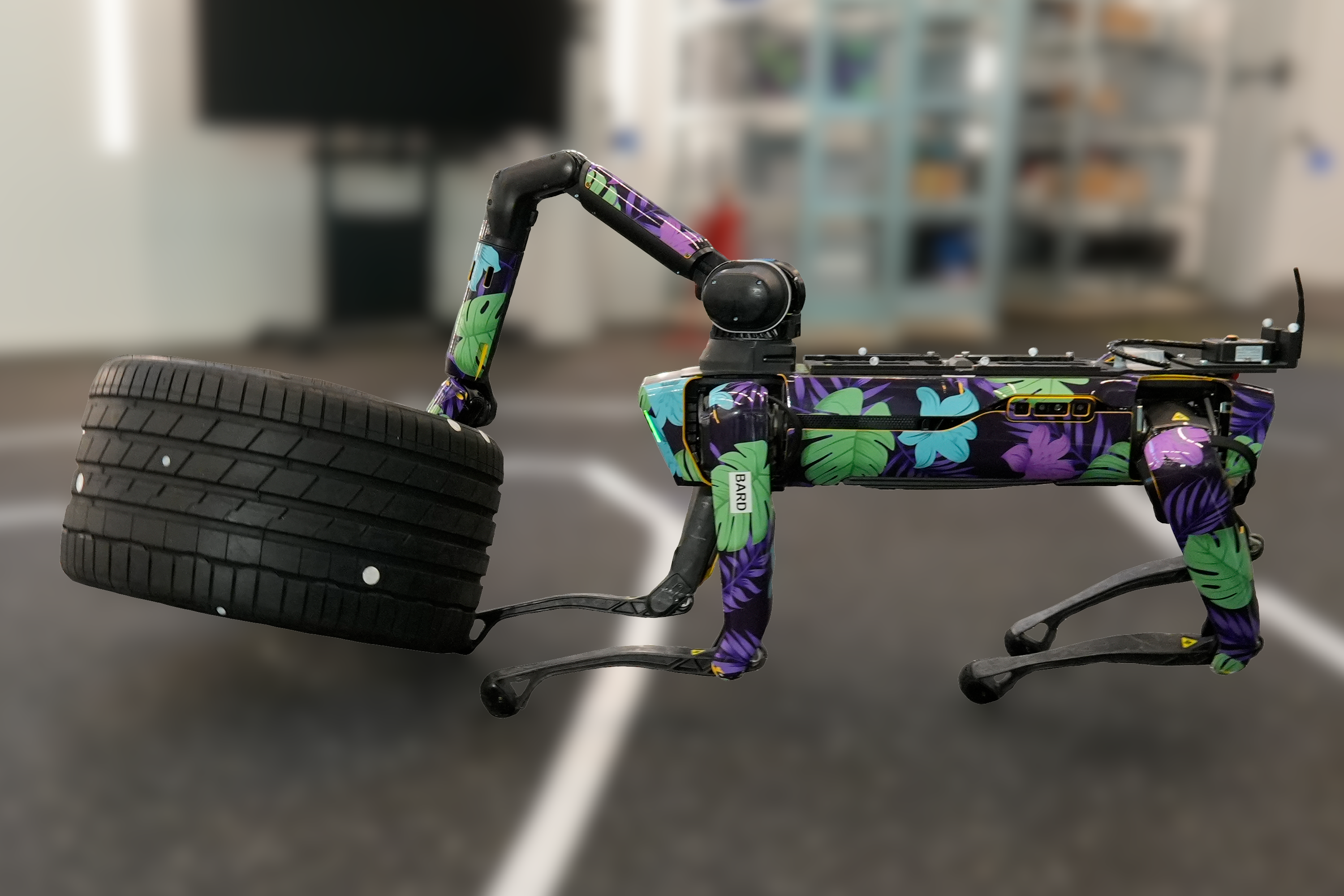
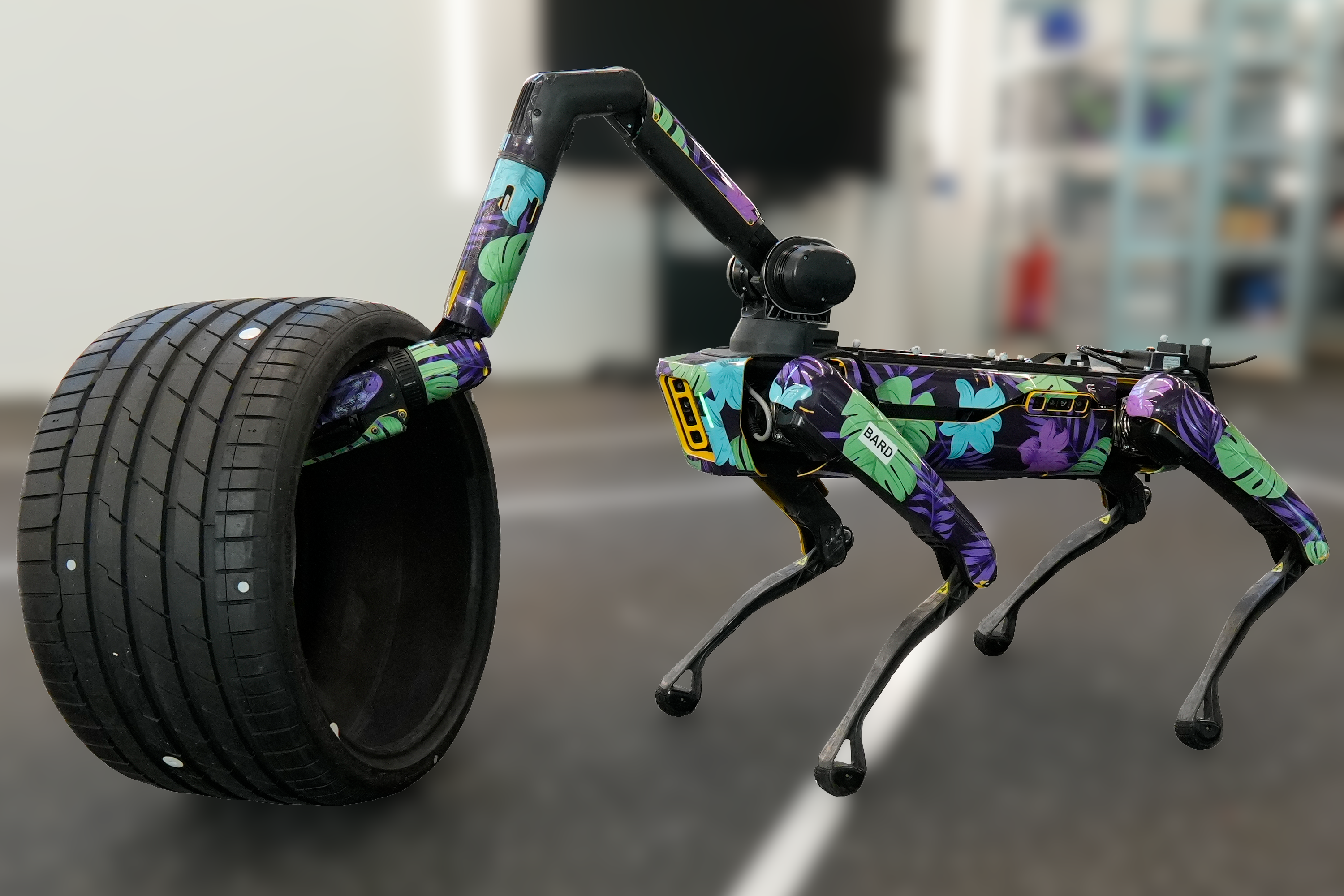
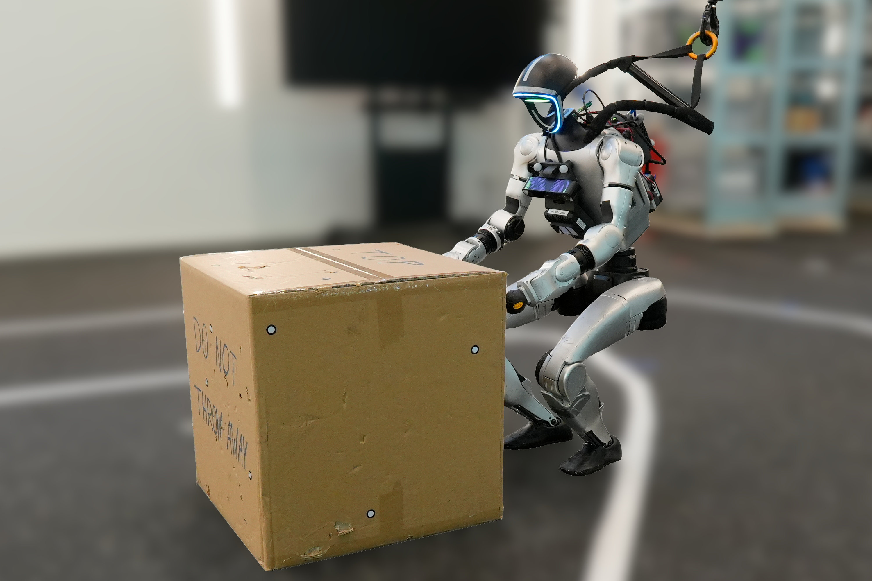
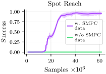
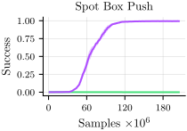
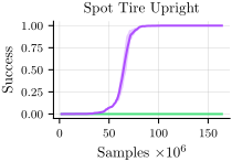
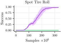
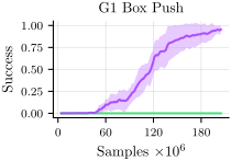
Five simulated tasks comprise Spot reaching, box pushing, tire uprighting, tire rolling, and G1 box pushing. Five-seed training curves approach high success with expert data, while sparse training without it fails on the complex tasks. Hardware Spot results are 10/10 reaching, 9/10 pushing, 10/10 uprighting, and 8/10 rolling. G1 deployment is demonstrated, but Table 1 does not provide the same ten-trial quantitative result for G1. These are state-based transfers with the specified controller and sensing setup.
| Reach | Box Pushing | Tire Uprighting | Tire Rolling |
| 10 / 10 | 9 / 10 | 10 / 10 | 8 / 10 |
Q1: Improving over seen expert data
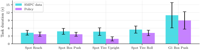
Trained policies finish the simulated tasks faster than the SMPC demonstrations, with some mean-time improvements exceeding 50% and reported duration-standard-deviation reductions of 11–45%. Planner statistics use the four-million-transition dataset, while learned-policy statistics use 50,000 simulated episodes without exploration noise. This supports improvement over the sampled teacher behavior, not globally optimal task execution.
Q2: Amount of data
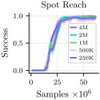
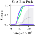
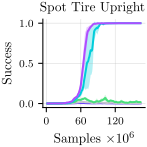
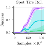
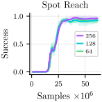
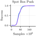
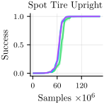
Simpler tasks tolerate substantially smaller expert datasets; coordinated tire manipulation benefits from millions of transitions and broader coverage. The authors attribute this to critic estimates becoming more reliable near useful states. Dataset coverage is a plausible explanation, but the experiment does not isolate it from all other effects of dataset size.
Q3: Quality of the data
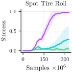
Reducing the number of sampled planner candidates lowers demonstration quality. Most tested tasks remain learnable, while tire rolling is more sensitive. The result suggests that acceptable teacher quality depends on coordination and precision demands, rather than requiring uniformly optimal demonstrations.
Q4: Multimodality in the data
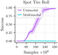
A tire dataset containing disparate strategies—leg kicks, body pushes, or stepping into the tire—fails to initialize the tested learner, even with slightly higher demonstration success. Planner contact penalties encourage a more consistent arm-based strategy and restore learning. This shows a limitation of the chosen dataset and learner combination; it is not evidence that Markov policies or offline RL inherently require unimodal data.
Q5: Training directly on the SMPC cost and data
Online FastTD3 with the planner’s dense costs, offline IQL, and Diffusion Policy all solve reaching but achieve at most 10% success on the harder Spot tasks under the tested setups. The proposed method reaches roughly 98–100% simulated success. These comparisons show that direct reuse of planner costs or imitation of its trajectories is insufficient here. The authors attribute imitation failures partly to missing recovery samples; that explanation is not independently tested with a full corrective-data study.
| Task | FastTD3 | IQL | DP | Ours |
|---|---|---|---|---|
| Reach | 1.00 | 1.00 | 1.00 | 0.98 0.03 |
| Box pushing | 0.00 | 0.03 | 0.10 | 0.99 0.005 |
| Tire uprighting | 0.00 | 0.01 | 0.01 | 1.00 0 |
| Tire rolling | 0.02 | 0.04 | 0.01 | 0.98 0.02 |
5 Conclusion
Planner demonstrations can make sparse-task-reward learning practical for coordinated whole-body skills and allow a compact policy to improve on its teacher. The main advantage is moving behavior specification into faster planner tuning and then using online RL for refinement. It still depends on a simulator, a successful teacher distribution, engineered control interfaces, and suitable learning hyperparameters.
6 Limitations
Behavioral improvement remains local to the demonstration distribution and is not expected to discover wholly different globally optimal strategies. Network size and learning rates still affect results. The frozen low-level controller cannot adapt to task-specific disturbances despite its generic disturbance training. Deployment uses state estimates; unstructured or outdoor operation would require visual learning or policy distillation into a perception-based system.
Acknowledgments
The authors thank Annika Wollschläger and Dario Bellicoso for help exporting policies and deploying them on G1.
Appendix A Extended Ablations
The extended ablations average five training seeds and show standard deviations. They study how expert-data scheduling and bounded value estimates influence convergence.
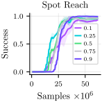
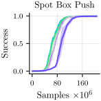
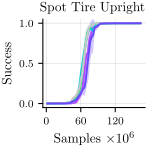
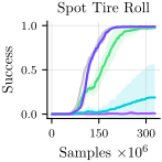
Percentage of Expert Data
Reaching, pushing, and uprighting are relatively insensitive to the initial expert fraction under the phase-out schedule. Tire rolling fails with too little expert data and benefits from higher initial fractions. Because expert data are removed after 10% success, any later benefit must arise through the learned initialization rather than continued access to those transitions.
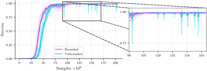
Bounded Critic Networks
At a deliberately increased critic learning rate of 8×10⁻⁴, both bounded and unbounded critics can converge on box pushing, but unbounded runs exhibit sharp performance drops. Bounding widens the stable hyperparameter range in this test; it does not remove the need for tuning or guarantee stability.
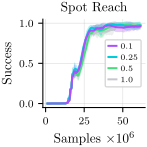
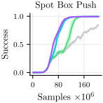
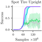
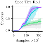
Phase-Out Threshold
Keeping planner data too long slows improvement once the learner begins succeeding. Thresholds at or above 50% prevent some tire-task runs from converging within the step budget; indefinite mixing is also harmful. The default removes expert data at 10% success. The proposed explanation is distribution mismatch between the increasingly specialized policy and the original teacher trajectories.
Appendix B RL Training Details
Training uses TD3 in mjlab/MuJoCo Warp with randomized object mass, size, and friction. The actor receives noisy observations while the critic receives exact simulated state. Rewards are scaled by 0.01, and action regularization and G1-specific learning-rate adjustments are retained. High-level learning takes 20–90 minutes on an RTX 5090, excluding expert-data generation and low-level-controller preparation. The original hyperparameter table specifies replay capacity, batches, update ratios, and other settings.
| Parameter | Value |
|---|---|
| Buffer size | |
| Gradient steps per update | |
| Phase-out threshold | |
| Batch size | |
| Discount factor | |
| Polyak factor | 0.005 |
| Actor learning rate | |
| Critic learning rate | |
| Policy delay | 2 |
| Smoothing noise | 0.05 |
| Action regularization | |
| Reward scale | 0.01 |
B.1 Bounding the Critic
Before reward scaling, the largest return is zero and the lowest is the immediate crash penalty −2/(1−γ). A final tanh, affine scaling, and initialization bias constrain critic predictions to that interval and start them near zero. This uses the deliberately simple reward’s known bounds rather than estimating limits from data.
Equation
Appendix C SMPC Data Collection
The planner broadcasts each initial state across a tile of simulation candidates, samples smooth spline action sequences, evaluates them, and selects the best. Warm starts shift the preceding best sequence; only the first ten actions are executed before replanning. The specified 50 Hz action rate yields 5 Hz replanning, with a 50-step horizon, ten spline control points, and 256 candidates per tile. State caching avoids redundant simulation. Algorithm 1 and Table 4 preserve the full collection procedure and parameters.
| Parameter | Value |
|---|---|
| Horizon | |
| Spline control points | |
| Frequency | |
| Execution steps | |
| Discount factor | |
| Samples per tile | |
| Minimum noise | |
| Maximum noise |
SMPC Tuning in Practice
Costs begin with goal distance and fall penalties, then add gripper proximity, contact restrictions, and smoothing as needed. Sliders support qualitative tuning while observing a few trajectories; each task reportedly takes less than an hour to tune. Data-generation times are 1h39m for reaching, 2h41m for box pushing, 3h28m for uprighting, 3h15m for rolling, and 10h06m for G1. This is rapid manual planner tuning, not the absence of task-specific design.
Appendix D Hardware Setup
Spot inference runs offboard with commands sent over WiFi; G1 inference runs on a mounted computer. OptiTrack tracks robots and objects alongside onboard sensing. The box is a 0.5 m cube weighing 1.2 kg; the tire has 0.33 m radius, 0.34 m width, and 14.3 kg mass. These controlled state-estimation and object conditions are material to the reported hardware transfer.