Overview
This edition covers the complete 48-page v1 dated 4 August 2026. It preserves all 37 figures and 11 tables, including the appendix diagnostics. Sparse factorization still requires optimization; the efficiency claim concerns calibration or optimizer-consumed tokens, not equivalent computation or the original dense model’s pretraining cost.
| Code: | github.com/veri-safe/SWD | Model: | huggingface.co/veri-safe/SWD | Blog: | huggingface.co/spaces/veri-safe/SWD-Blog |
At a glance
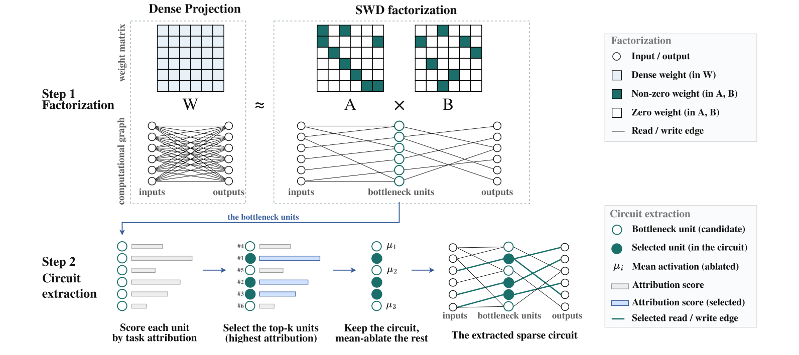
Sparse Weight Decomposition (SWD) approximates each pretrained linear projection by two sparse factors. Their intermediate coordinates become individually addressable read–write paths for circuit ranking and ablation. Single-matrix experiments report high replacement fidelity with much less fitting data than learned replacements, and smaller task circuits in active-edge cost. Fixed-support finetuning extends the method to GPT-2’s transformer body; a weight-only variant omits calibration activations. These are local, protocol-dependent explanations, with explicit exceptions to fidelity matching and limited large-model coverage.
1 Introduction
Dense model weights distribute task behavior across many coordinates. SWD obtains sparse intermediate paths by repurposing Double Sparse Factorization rather than learning a separate activation dictionary. Unlike exact dense SVD components, each path has few nonzero incoming and outgoing weights. Experiments separate replacement fidelity from the cost of the subsequently selected task circuit, and test single matrices, GPT-2’s whole transformer body, exact dense controls, weight-only fitting and qualitative interventions.
2 Methodology
The method first constructs sparse factors, then applies a common task-based circuit extraction and evaluation protocol to their intermediate units.
2.1 Sparse Weight Decomposition
A bottleneck unit is a scalar intermediate activation coupled to sparse input and output directions. The factorization changes the model approximately, so replacement quality must be checked before interpreting its circuits.
Sparsity on the edges.
Sparsity is imposed on both read and write weights. Exact dense factorizations also expose intermediate units, but each normally touches almost every input/output coordinate. The controls test whether sparse connectivity reduces circuit cost beyond this change of basis.
Objective.
For W of shape input-width × output-width, SWD fits A and B under a fixed combined nonzero budget K. Calibration-weighted squared reconstruction error prioritizes activation directions the model encounters; setting the activation Gram matrix to identity yields the weight-only Frobenius objective. Larger reported sparsity means fewer surviving factor entries. The original derivation is retained below; its matrix quadratic form needs a trace to equal the scalar squared-error objective, although the printed expression omits it.
Equations
Solver.
The nonconvex sparsity-constrained problem is approximated with the DSF solver: alternate factor updates using regularized least squares, hard thresholding and ADMM dual updates. Local finalization freezes supports and A, then refits B. When all projections are replaced, a separate next-token finetuning stage updates existing nonzero values in both factors while keeping supports and other pretrained parameters fixed.

Selectable original takeaway
2.2 Circuit Extraction from Sparse Factors
Each intermediate scalar multiplies one write row, so the reconstructed output is an additive sum of read–write paths. Rank units by positive task-margin attribution on training examples. To test sufficiency, keep the selected paths and replace all others by their training-split mean activations; to test necessity, mean-ablate the selected paths and retain the remainder. Mean ablation preserves average activation levels while removing input dependence. Independent addressability does not imply functional independence across nonlinear computations.
Equations

Selectable original takeaway
3 Experiments
Experiments compare fidelity before pruning and the minimum circuit cost needed to attain held-out sufficiency or necessity targets. Large-model studies replace one projection; whole-body replacement is evaluated on GPT-2 Small.
3.1 Baselines
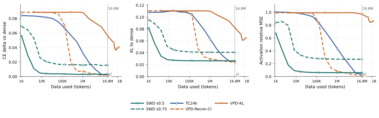
Transcoders learn sparse activation features; VPD learns parameter components with an input-dependent causal-importance selector; sparse pretraining trains a separate sparse model. VPD-KL uses output-distribution KL, whereas VPD-Recon-CI changes the fidelity term to local reconstruction. VPD-KL fails the required fidelity match and is shown only for replacement quality. The sparse-pretraining comparison is confined to the whole-model experiment.
| Property | SWD (ours) | Transcoder | VPD | Sparse pretrain |
|---|---|---|---|---|
| Separate model training (additional optimization cost) | No; fit sparse factors post hoc | Yes; train a replacement network for the pretrained model | Yes; train a decomposition and input-dependent selector for the pretrained model | Yes; train the complete sparse model from scratch |
| Representation and unit of analysis | Two sparse factors; one bottleneck unit is a rank-one read–write path | A replacement network; one unit is a hidden feature | A parameter decomposition; one unit is a rank-one parameter component | A sparse pretrained model; one unit is a native hidden channel |
| Type of sparsity | Weight sparsity in the factor matrices | Activation sparsity in hidden features | Input-dependent component selection over parameter components | Weight sparsity throughout the model; activation sparsity is disabled in our run |
| Optimization objective | Reconstruct target weights or their outputs on calibration data under fixed factor sparsity | Reconstruct original MLP outputs while encouraging sparse feature activations | Match model outputs or replaced-matrix outputs, with parameter reconstruction and sparse component use | Minimize language-model loss while progressively sparsifying weights |
| Data required | None or a small amount of calibration data* | Text used to train the replacement network | Text used to train the decomposition and selector | Full pretraining corpus |
| Applicable scope | MLP and attention matrices; from one matrix to all model projections | MLP computations; one MLP at a time in our comparisons | MLP and attention matrices; from one matrix up to full-model replacement | Whole model during pretraining |
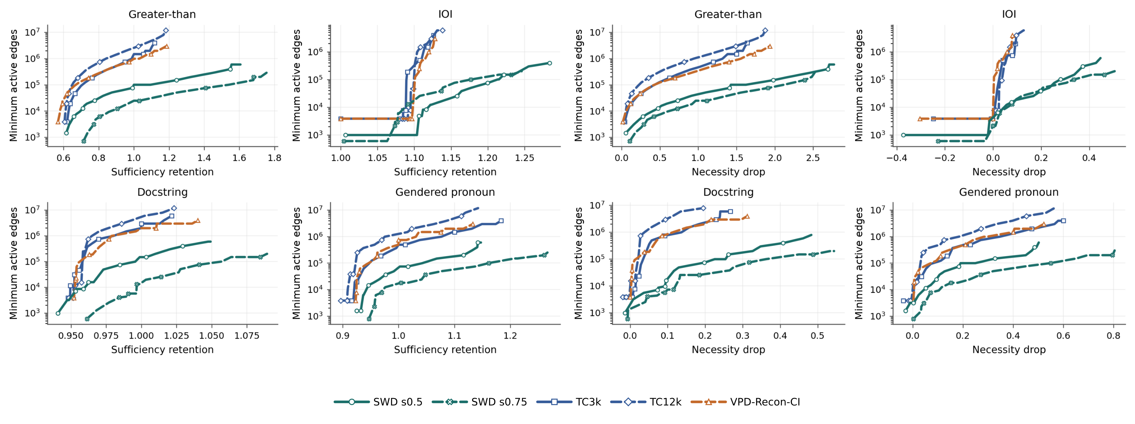
*At matched replacement CE, SWD uses less than 1% of the data used by the corresponding trained baseline in our experiments. This greater data use does not consistently reduce circuit cost: SWD typically reaches the same sufficiency or necessity target with fewer active edges; see Sections 3.3 and 3.4.
3.2 Evaluation Protocol
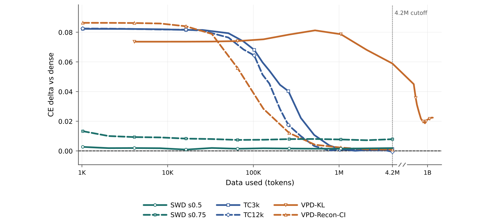
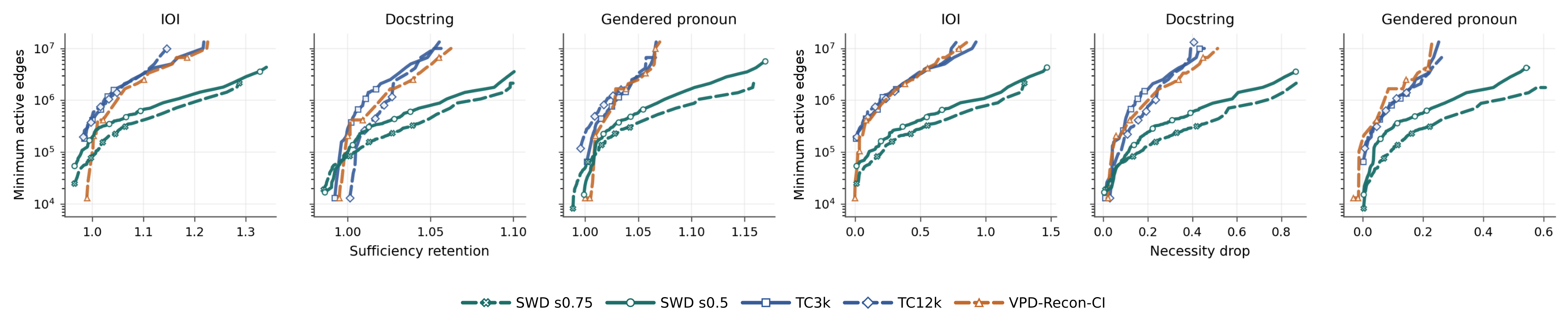
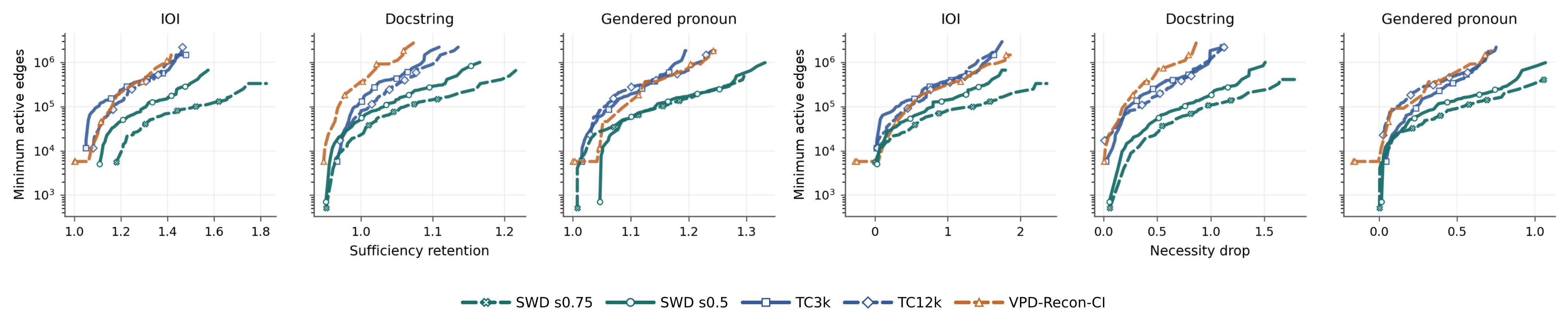
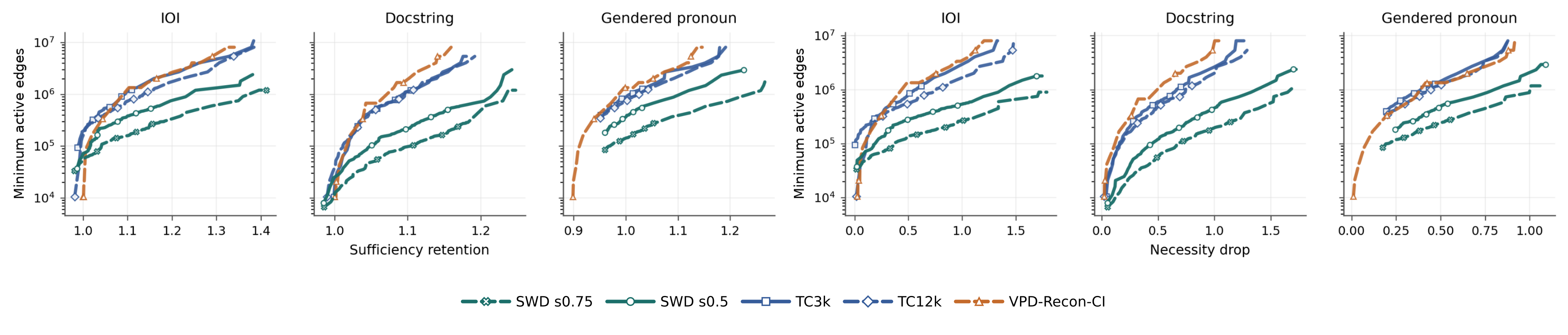
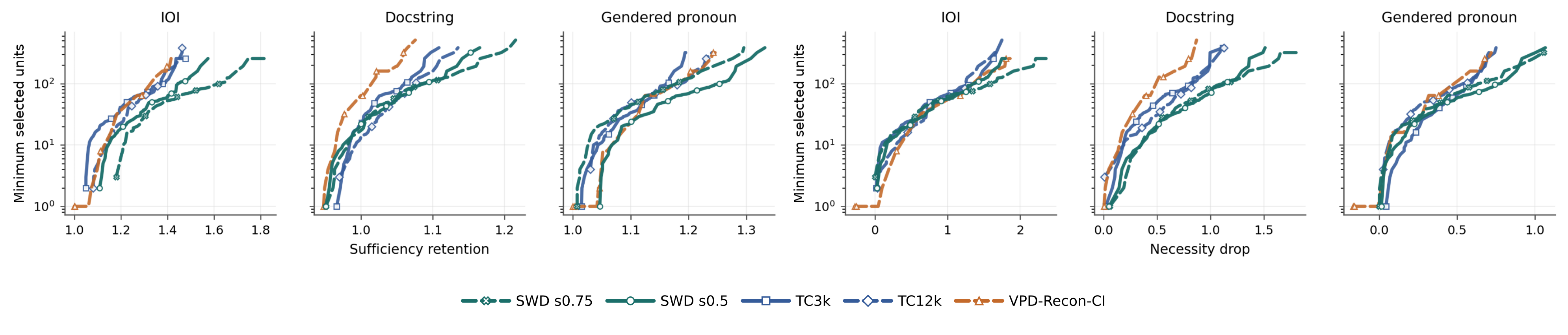
FineWeb-Edu supplies fitting data and a disjoint fidelity test split. Circuit tasks use separate train/test examples: train estimates positive first-order attribution and ablation means; held-out test evaluates fixed nested top-k sets. Sufficiency is retained task margin divided by the unpruned replacement’s margin; necessity is its margin minus the selected-unit-ablated margin. Cost is selected units or nonzero read/write edges of valid selected paths. Curves take the minimum cost among evaluated prefixes reaching each target. The usual CE tolerance is .001, but stated controls and some 27B curves exceed it; matched average CE also does not imply identical predictions. Intervention choice can affect circuit conclusions.
Equations
3.3 Single-Matrix Replacement
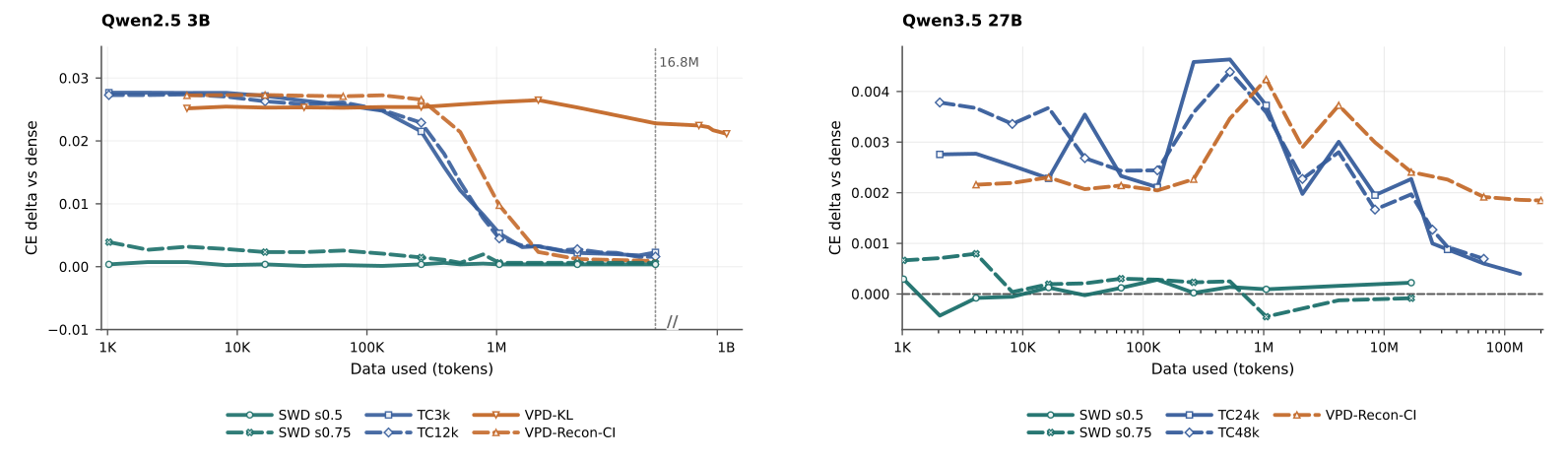
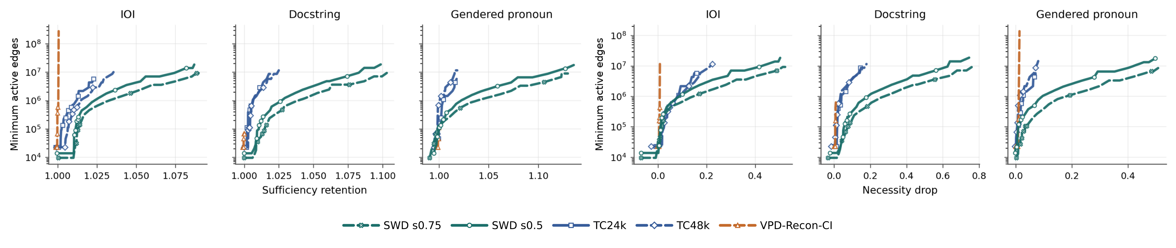
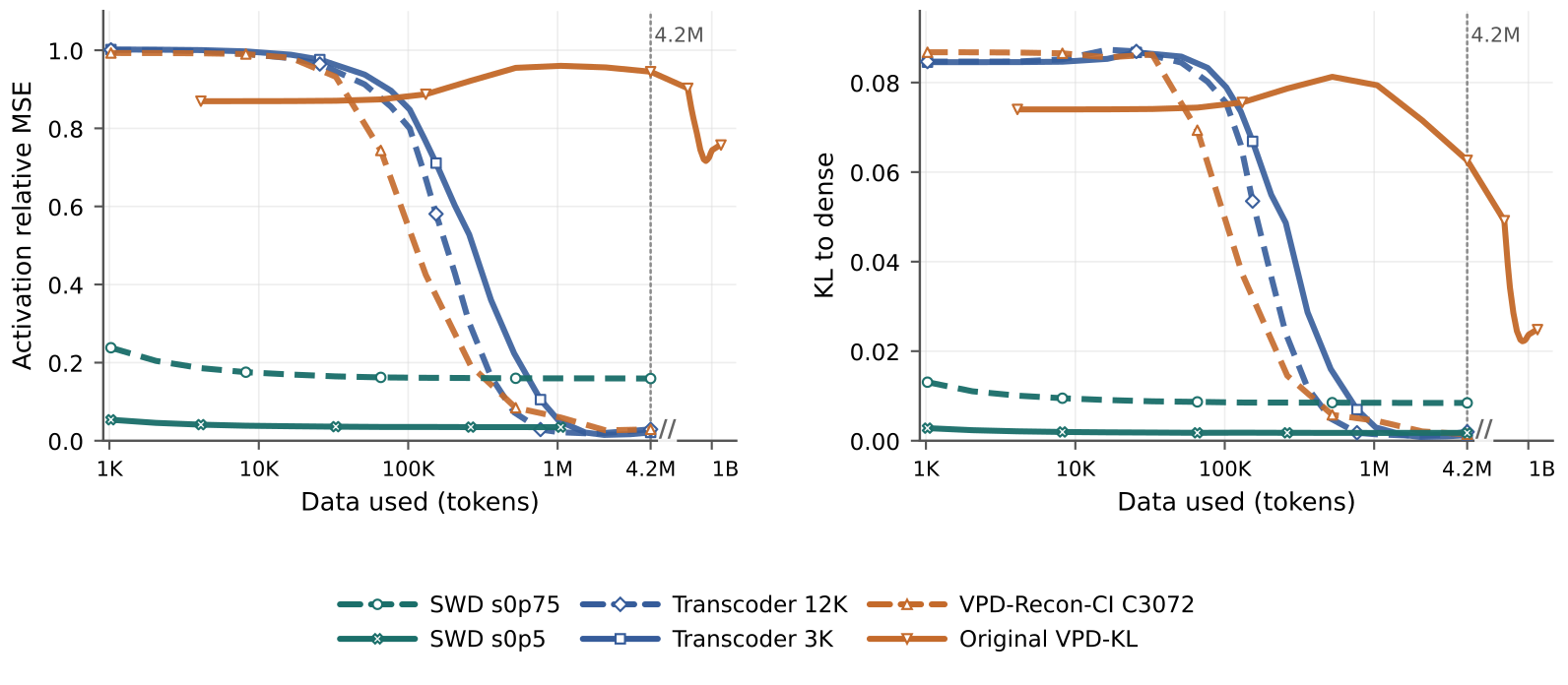
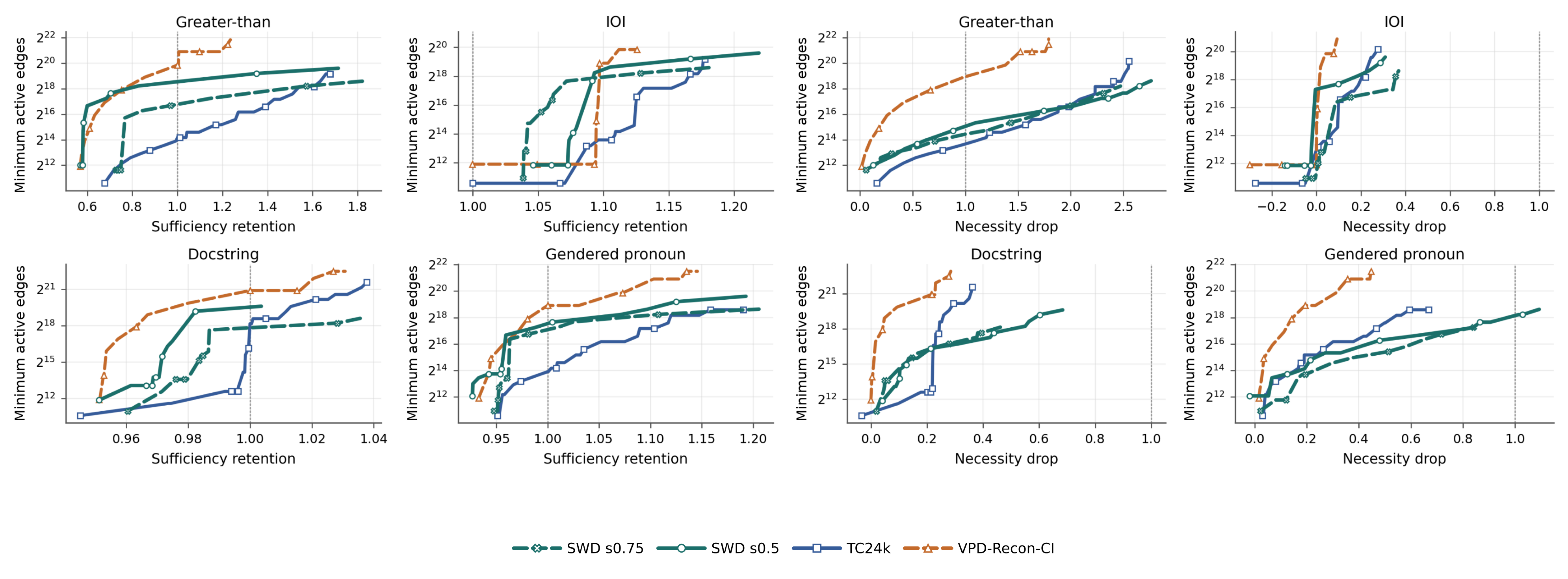
For GPT-2 layer-8 output projection and Qwen down projections, SWD reaches low error with fewer fitting tokens and generally needs fewer active circuit edges than the trained replacements. The main matched comparison uses sparsity .5; sparsity .75 usually trades fidelity for fewer edges. GPT-2 zero-ablation controls retain the cost advantage with rankings fixed. Qwen3.5-27B confirms feasibility for one matrix, with TC48k and VPD-Recon-CI outside the stated matching tolerance. Whole-MLP replacement gives more mixed results, including competitive Transcoder sufficiency and unit counts.

Selectable original takeaway
3.4 Full-Model Replacement
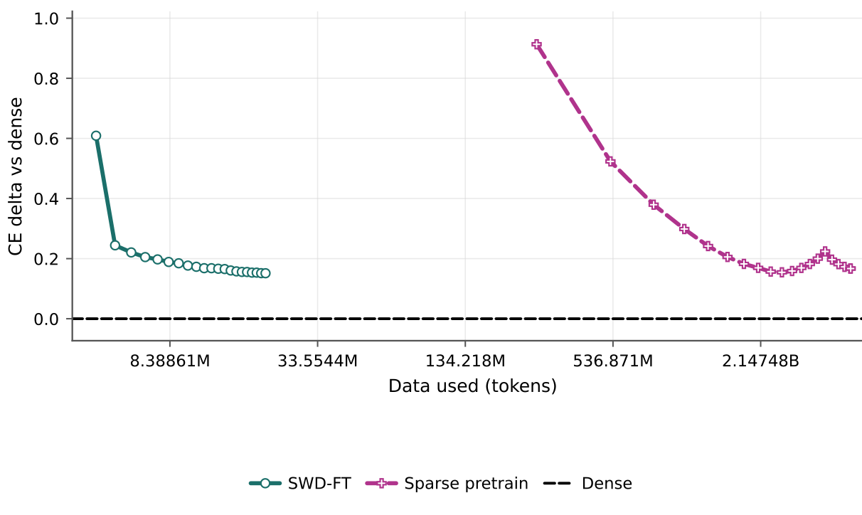
Replacing all 48 attention/MLP matrices across GPT-2’s twelve blocks gives CE 3.90 before finetuning and 3.44 after fixed-support finetuning, versus 3.45 for a separate sparse-pretrained model at approximately 26.77M active body weights. SWD uses 4.19M calibration plus 16.38M finetuning token presentations, versus 2.884B sparse-pretraining presentations. This excludes inherited dense pretraining and is not a FLOP comparison. Circuit results are broadly comparable on GreaterThan/gendered pronouns; sparse pretraining has near-zero or negative necessity drop on docstring/IOI. Its circuit candidates and activation implementation also differ, as detailed in B.5.3.
| Method | Data used | Active nonzero weights | LM CE loss |
|---|---|---|---|
| SWD | M calibration tokens | M | |
| SWD-FT | M calibration + M fine-tuning tokens | M | |
| Sparse pretrain | B sparse-pretraining tokens | M |
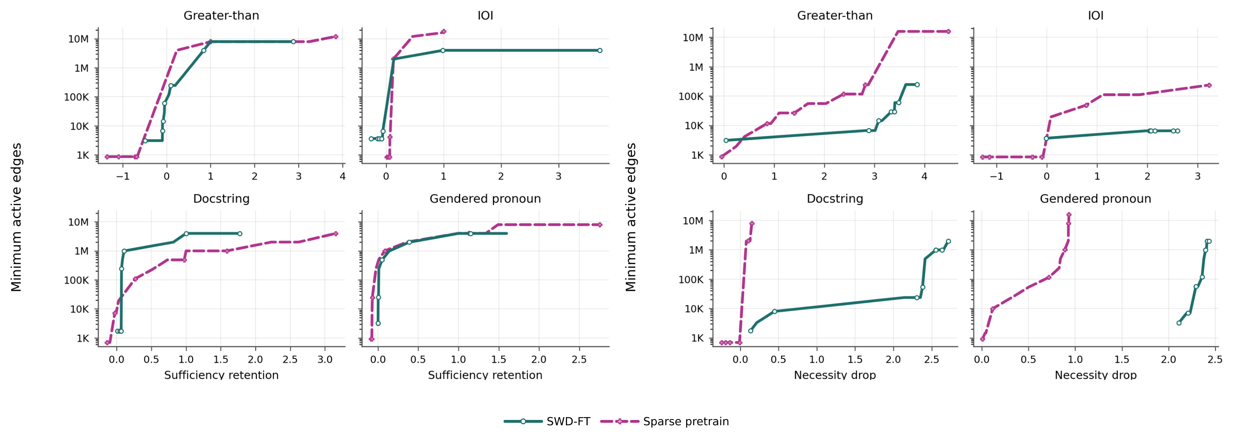

Selectable original takeaway
3.5 Ablation: Exact Dense Reparameterizations
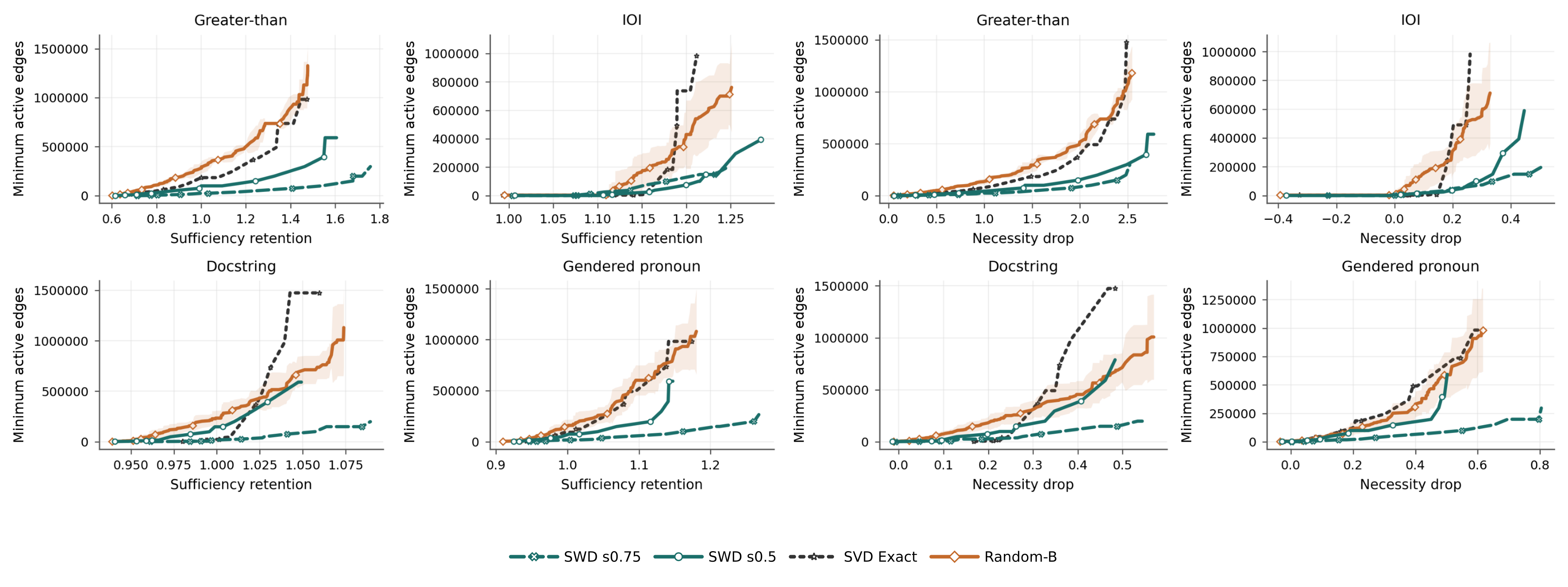
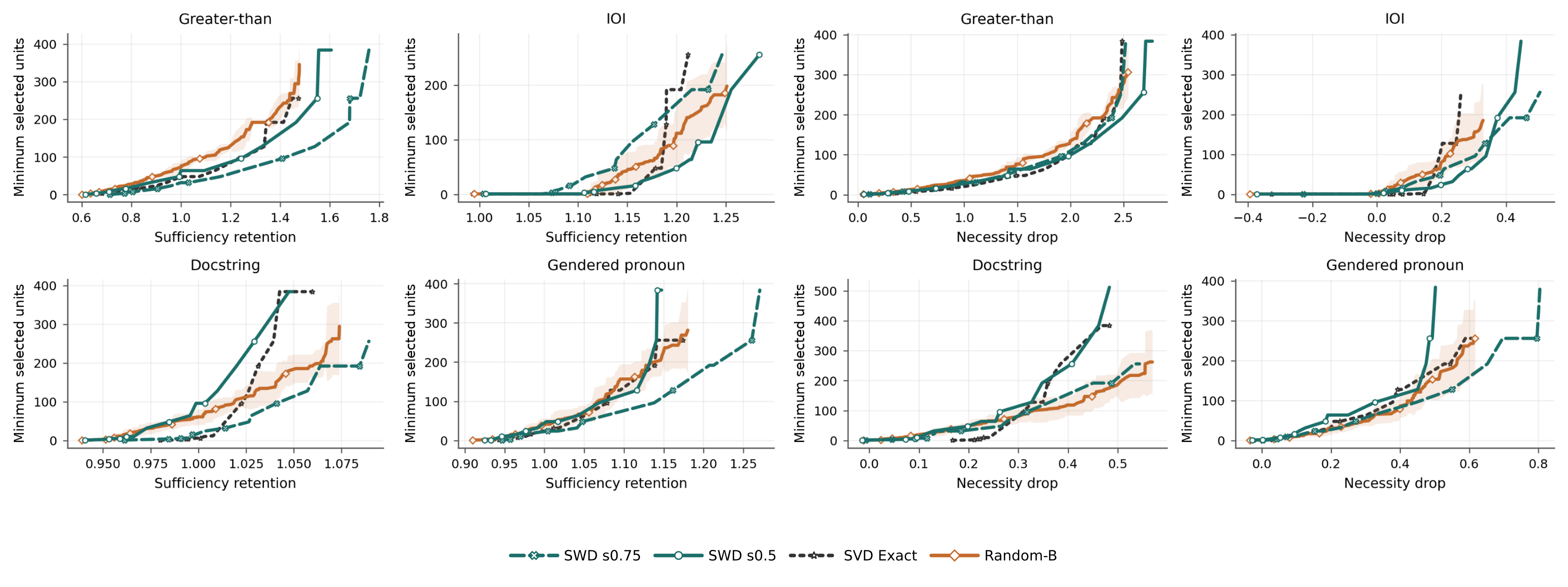
Full-rank SVD and seeded random-orthogonal factorizations reproduce the dense target exactly, yet need more read/write edges for similar circuit targets. This isolates sparse connectivity from factorization alone under the shared ranking/ablation protocol. Dense controls remain competitive in some selected-unit comparisons; the clearer advantage is active-edge cost.

3.6 Zero-Data Factorization
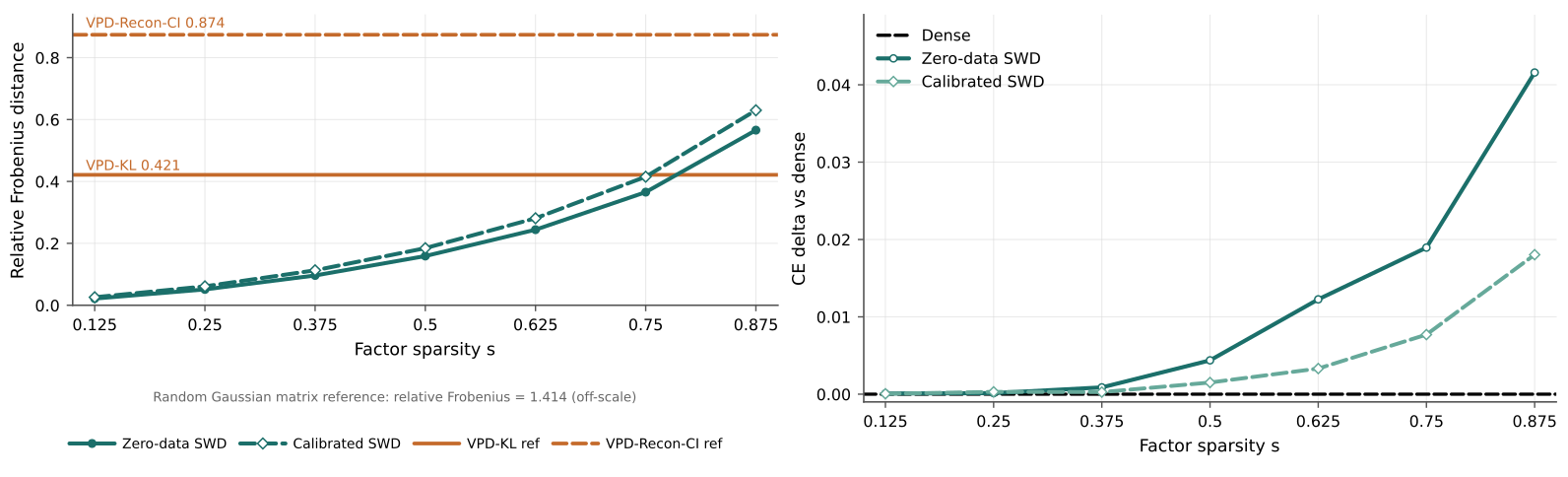
Weight-only SWD sets the Gram matrix to identity and uses no calibration text to fit factors. It preserves the raw matrix more accurately: at sparsity .75 its relative Frobenius error is .366 versus .415 for calibrated SWD. Calibration instead better preserves held-out CE under aggressive sparsity. Task circuits remain useful, but their ranking, ablation statistics and evaluation still require task data. Tracking circuits across training checkpoints is proposed future work.

Selectable original takeaway
3.7 Qualitative Results
The qualitative studies examine semantic hypotheses, a directional weight edit, one attention intervention and pair interactions. They illustrate possible uses of the representation rather than establish general monosemanticity or complete mechanistic understanding.
3.7.1 Semantic Audit of a Task Circuit
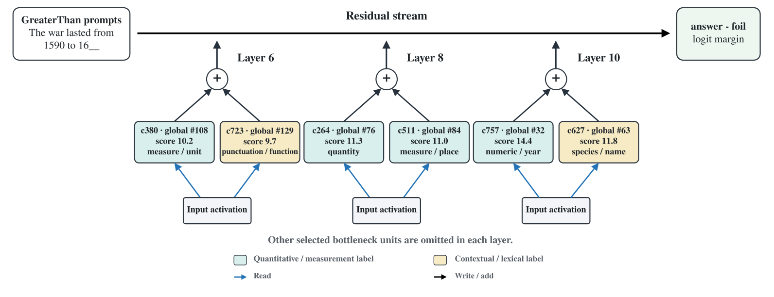
Rank 9,208 valid all-layer GPT-2 output-projection units by GreaterThan attribution. The six displayed units are the top two in layers 6, 8 and 10 and lie within the global top 512. Twenty strongest activation contexts per unit, drawn from 2,048 independent WikiText-2 tokens, support four number/quantity/measurement hypotheses and two contextual lexical/syntactic hypotheses. Appendix H specifies model-generated labeling.
3.7.2 Targeted Bottleneck-Unit Editing
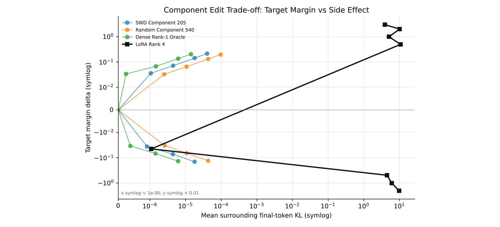
All edits start from the same original dense layer-8 output matrix. Unit c205 supplies a read direction for a rank-one update toward “down” rather than “left” on “The opposite of up is”. Its largest positive setting changes the final margin by .216 with mean KL 4.02×10⁻⁵ on seven unrelated prompts. It improves measured locality over the selected random-unit and rank-4 LoRA controls; a target-conditioned dense oracle is stronger. This is one screened target and a small probe set.
3.7.3 Mechanistic Diagnostics
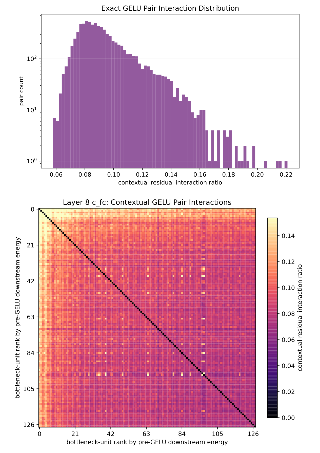
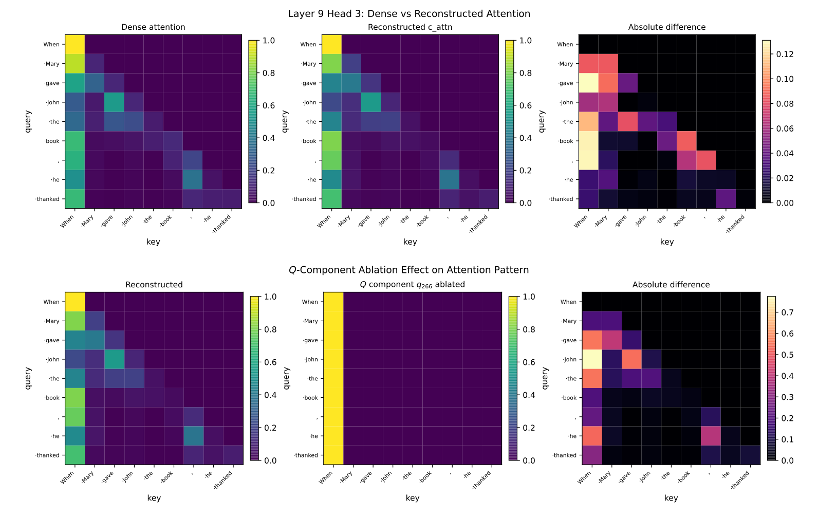
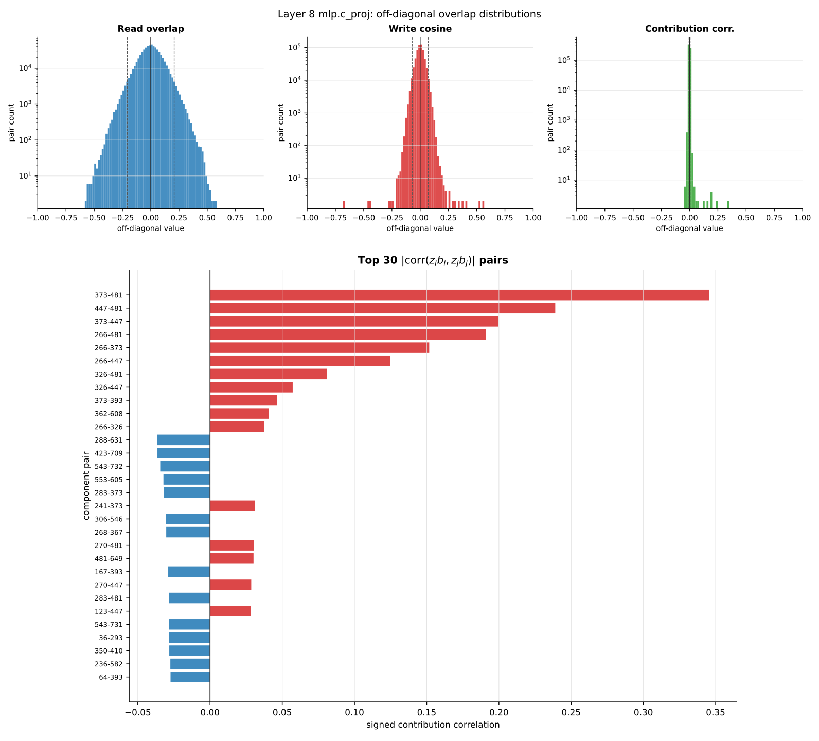
Static query/key geometry selects candidates for prompt replay and intervention. In the highlighted layer-9/head-3 example, reconstructed attention has KL .0405 from the dense head; ablating q266 produces KL 2.496 from the reconstruction and maximum probability change .775. Separate diagnostics find mostly weak post-GELU contribution correlations but broader pre-GELU nonlinear interactions. Additive paths should therefore not be treated as mutually independent mechanisms.

Selectable original takeaway
4 Related Work
Prior work supplies the circuit tests, learned-feature and parameter-space alternatives, sparse-model motivation and factorization solver used here.
Task-level circuit discovery and evaluation.
ACDC, attribution patching and edge pruning search existing computation graphs. SWD instead introduces a new basis of intervenable paths inside dense linear maps; these selection algorithms can then operate on that basis. Held-out behavior and intervention definitions matter more than agreement with one presumed canonical circuit.
Sparse activation features and learned replacement modules.
Sparse autoencoders learn activation dictionaries, while Transcoders approximate MLP input/output computations with sparse features. SWD fits sparse weight factors applicable to both attention and MLP projections. Its units are parameter-side rank-one paths, without assuming each has a single semantic meaning.
Parameter-space interpretability.
APD, SPD and VPD learn parameter components and sparse per-input use. NaNA interprets exact SVD components as detector–effector units. SWD constructs sparse read/write components independently of the downstream circuit task, then applies task-margin ranking.
Sparse models and post-training pruning.
Post-training pruning removes scalar weights; sparse pretraining changes connectivity while training a model. SWD adds explicit intermediate units to a pretrained checkpoint, enabling path-level selection and ablation. The whole-model and exact-factor controls probe related but distinct sources of circuit sparsity.
Matrix factorization and compression.
Matrix compression has long used low rank, nonnegativity and sparsity. SWD adopts Double Sparse Factorization and activation calibration, then evaluates the resulting units for circuit extraction. Its contribution is this interpretability application and evaluation, not a new DSF optimization algorithm.
5 Limitations
Cheaper extraction narrows one practical bottleneck, while replacement fidelity, non-uniqueness and verification remain unresolved.
Efficient extraction is not complete understanding.
Small circuits affecting held-out task margins do not provide a global account of the model or guarantee coverage of rare safety-relevant behavior. Reduced fitting data and circuit edges do not settle the broader limits of mechanistic interpretation.
SWD circuits are local and non-unique.
The approximate factors are not established as identifiable; units can depend on calibration, initialization, objective and sparsity, in addition to scaling/permutation symmetries. Average reconstruction/CE may hide input-specific drift. First-order ranking can miss important mechanisms, and ablation, pruning thresholds and graph granularity change conclusions. Treat results as task- and protocol-specific causal explanations, not unique ground truth.
Scaling verification remains open.
The 27B experiment covers one matrix, whole-model replacement covers GPT-2 Small, and the semantic audit shows six labeled units. Broader decompositions, prompts and adversarial edge cases need independent verification. SWD complements behavioral and representation-level analysis rather than certifies understanding or safety.

6 Conclusion
Sparse read/write factorization makes compact local circuit hypotheses available directly from pretrained weights. Fidelity checks, fixed-support finetuning and causal task tests make these paths useful analytical objects, while the controls attribute much of the edge-cost advantage to sparse connectivity. General interpretation remains limited by approximate replacements and interacting, non-unique units.
Appendix A Notation
The complete notation table remains below. Layer/head/unit indices are zero-based; displayed attribution ranks are one-based. A valid unit has at least one nonzero read and write edge. “Unit” encompasses SWD bottlenecks, Transcoder features, VPD components and sparse-pretrained latent channels.
| Symbol | Meaning |
|---|---|
| Dense target weight matrix and its SWD replacement, . | |
| Sparse read and write factors, and . | |
| Input and output dimensions of the target matrix. | |
| Numbers of SWD bottleneck units and VPD component slots, respectively. | |
| indexes a candidate unit; is the number of highest-ranked units retained in a top- circuit. | |
| Input text example and the input activation to target module at token position . | |
| Calibration-activation matrix whose rows are input-activation vectors . | |
| Calibration Gram matrix and the identity matrix used by the zero-data objective. | |
| Total factor-entry budget and factor sparsity . | |
| Distribution of calibration activations used to fit SWD. | |
| Training and held-out evaluation splits for circuit task . | |
| Activation of unit , its train-split mean used for ablation, and its task-attribution score. For SWD, . | |
| is the set of the highest-ranked units; contains the selected units with at least one nonzero read edge and one nonzero write edge. | |
| Method-specific read and write weight vectors of unit ; for SWD these are and . | |
| Selected-unit cost and active-edge cost . | |
| Replacement model before circuit pruning. | |
| Models that respectively retain only or mean-ablate . | |
| Per-example answer-versus-distractor logit margin for task . | |
| Average task margin of model over split . |
Appendix B Experimental Details
Fitting and fidelity evaluation use disjoint language-model data. Circuit rankings and ablation means are trained once and fixed before held-out circuit evaluation. Replacement surfaces, token accounting and baseline checkpoint choices remain explicit.
B.1 Models and Replacement Targets
Table 4 identifies each exact replacement surface: GPT-2 layer-8 output projection, middle Qwen2.5 down projections, Qwen3.5 layer-31 down projection, GPT-2 layer-8 complete MLP, or all 48 GPT-2 body matrices. Single-matrix comparisons share the same target within each model.
| Setting | Model | Replacement surface |
|---|---|---|
| GPT-2 single matrix | GPT-2 Small | Layer 8 mlp.c_proj |
| Qwen2.5 scaling | Qwen2.5 0.5B, 1.5B, 3B | Middle-layer mlp.down_proj: layers 12, 14, and 18, respectively |
| Qwen3.5 single matrix | Qwen3.5-27B | Layer 31 mlp.down_proj |
| GPT-2 MLP replacement | GPT-2 Small | Layer 8 standard MLP, comprising mlp.c_fc and mlp.c_proj |
| GPT-2 full-model replacement | GPT-2 Small | attn.c_attn, attn.c_proj, mlp.c_fc, and mlp.c_proj in all 12 blocks |
| Zero-data | GPT-2 Small | Layer 8 mlp.c_proj, matching the GPT-2 single-matrix experiment |
| Qualitative audit | GPT-2 Small | mlp.c_proj in all 12 blocks; selected bottleneck units are visualized from layers 6, 8, and 10 |
B.2 SWD Factorization and Fixed-Support Fine-Tuning
Default inner width is the smaller matrix dimension. Square-factor density is .16 for square targets and .25 for rectangular ones; the other factor receives the remaining nonzero budget. Gram-diagonal rescaling precedes identity/pruned-target initialization. GPT-2 uses forty outer alternations, Qwen eight; each factor update has five ADMM iterations with ridge .01, initial support changes for two iterations and scheduled penalty. Twenty final fixed-support iterations refit one factor. Each calibration-curve point is independently fitted, not a successive checkpoint; Table 5 records exact data/CE settings.
| Experiment | CE-curve data (tokens) | Fixed replacement used for circuit extraction |
| GPT-2 single matrix | 1,024–4.19M | : 16,384 tokens; CE delta |
| : 16,384 tokens; CE delta | ||
| Qwen2.5-0.5B | 1,024–33.55M | : 1,024 tokens; CE delta |
| : 1.05M tokens; CE delta | ||
| Qwen2.5-1.5B | 1,024–33.55M | : 1,024 tokens; CE delta |
| : 1.05M tokens; CE delta | ||
| Qwen2.5-3B | 1,024–33.55M | : 2,048 tokens; CE delta |
| : 1.05M tokens; CE delta | ||
| Qwen3.5-27B | 1,024–16.78M | : 2,048 tokens; CE delta |
| : 1.05M tokens; CE delta | ||
| GPT-2 MLP replacement | 1,024–33.55M | : 16,384 tokens; CE delta |
| : 16,384 tokens; CE delta | ||
| GPT-2 full model | 4.19M (factorization) + 16.38M (fine-tuning) | Final SWD-FT replacement (20.57M total tokens) |
| Zero-data SWD | 0 | Fixed zero-data factors at each evaluated sparsity |
Equation
Circuit cost.
SWD cost counts nonzeros in a selected column of A plus its row of B. Whole-model finetuning freezes the 26,770,800-entry support and all other pretrained parameters. It uses 4.19M unique tokens replayed for 2,000 steps at batch eight, totaling 16.38M presentations. AdamW peaks at 5×10⁻⁷ with betas (.9,.95), epsilon .1 and decay .001; one-percent warmup precedes linear decay. Global factor-gradient RMS is normalized to one; training uses bfloat16, evaluation float32 and seed zero.
B.3 Unit Scoring and Circuit Selection
Score each candidate under the unpruned replacement by the training-set expectation of the positive part of activation times task-margin gradient. Means are also estimated on this split. One descending ranking defines every top-k prefix; neither rankings nor ablation means are refitted on test data. This common scoring procedure follows attribution patching.
Equations
B.4 Data Sources and Splits
Language-model fitting/evaluation and circuit-task scoring/evaluation are separate datasets with distinct accounting.
B.4.1 Language-Model Data
FineWeb-Edu supplies fitting data and fixed disjoint test data shared within comparisons. “Data used” means calibration tokens for SWD and optimizer-replayed tokens for trained replacements. Weight-only factorization uses no text; this does not remove task-data requirements for circuit testing.
B.4.2 Circuit-Task Data
Public Edge-Pruning and auto-circuit examples supply train/test splits retained in Table 6, including repository revisions. GPT-2 uses GreaterThan, IOI, docstring and gendered pronouns. Qwen omits GreaterThan because numerical answers violate the single-token scoring protocol; 27B examples are additionally filtered for tokenization compatibility. Circuit examples are excluded from replacement-fitting token counts.
| Task | Public source | GPT-2 | Qwen2.5 | Qwen3.5-27B |
|---|---|---|---|---|
| Greater-than | Edge-Pruning, a918efd8 | 80,000 / 12,240 | Not used | Not used |
| IOI | auto-circuit, 8fc5afd8 | 600 / 200 | 600 / 200 | 600 / 200 |
| Docstring | auto-circuit, 8fc5afd8 | 600 / 200 | 600 / 200 | 600 / 200 |
| Gendered pronoun | Edge-Pruning, a918efd8 | 3,024 / 378 | 3,024 / 378 | 2,887 / 370 |
B.5 Baseline Configurations
Baseline data axes compare consumed tokens, not optimizer steps, FLOPs or wall time. The usual maximum pre-pruning CE difference is .001; explicit reference curves remain visible when that match fails.
B.5.1 Transcoder
Transcoders expose sparse hidden features for the same replacement surface. Width, feature sparsity and checkpoint choices determine the plotted configurations.
Circuit cost.
A selected feature costs its nonzero incoming encoder plus outgoing decoder weights.
GPT-2 single-matrix replacement.
GPT-2 layer-8 c_proj uses widths 3,072/12,288, L1 coefficient 5×10⁻⁵ and seed 42. Curves cover 1,024–4.19M training tokens. Both circuit checkpoints use 2.048M tokens, with CE deltas .000529/.000979.
Qwen2.5 down-projection scaling.
Qwen2.5 .5B/1.5B/3B targets layers 12/14/18. Widths remain 3,072/12,288 with the GPT-2 penalty/seed; trajectories reach 33.55M tokens. Circuit checkpoints generally use 25.17M tokens, except 1.5B TC3k at 33.55M. Their CE deltas are .001654/.002032, −.000057/−.000098 and .001516/.001229 respectively.
Qwen3.5-27B down projection.
Qwen3.5-27B layer-31 down projection uses widths 24,576/49,152, penalty 5×10⁻⁵ and seed 42. Circuit checkpoints consume 134.22M/67.11M tokens and have CE deltas .000398/.000695. TC48k is slightly outside the .001 difference tolerance relative to SWD.
GPT-2 MLP replacement.
The complete GPT-2 layer-8 MLP Transcoder has width 24,576, L1 coefficient 1.4×10⁻⁴ and seed 42. Its only circuit checkpoint uses 6.29M tokens with CE delta .003456; Appendix E preserves the full quality trajectory.
B.5.2 VPD-KL and VPD-Recon-CI
VPD-KL and VPD-Recon-CI share the parameter components and learned causal-importance selector. Their fidelity losses differ: final next-token KL versus local elementwise reconstruction MSE, respectively. Selector minimality is separately regularized. VPD-KL remains a quality reference when it cannot match CE.
Equation
Circuit cost.
Cost counts a selected component’s nonzero read/write weights. The causal-importance predictor is excluded from this structural edge count.
GPT-2 single-matrix replacement.
GPT-2 c_proj VPD-Recon-CI uses 3,072 components, a width-128 selector, seed zero and minimality coefficient 10⁻⁴. Its fixed 4.19M-token checkpoint has CE delta .000873 and is reused for fidelity and circuit evaluations.
Qwen2.5 down-projection scaling.
Qwen2.5 uses 12,288 components and local reconstruction on layers 12/14/18. Circuit checkpoints consume 16.78M/4.19M/16.78M tokens for .5B/1.5B/3B, with CE deltas .000729/.001186/.000906.
Qwen3.5-27B down projection.
The 27B VPD reference uses 12,288 components, width-12 selector, seed zero and minimality coefficient 3×10⁻⁴. Its 200M-token checkpoint has CE delta .001847, outside the stated tolerance relative to SWD; it remains a parameter-decomposition reference.
GPT-2 MLP replacement.
Complete-MLP VPD-Recon-CI uses 3,072 components; its circuit checkpoint consumes 4.19M tokens with CE delta .003522. The native-KL version uses 3,072 components/seed zero and extends to one billion tokens for replacement quality only.
B.5.3 Sparse-Pretrained Reference
The sparse-pretraining baseline is a separately trained GPT-2-shaped model, not a sparse replacement of the Hugging Face checkpoint inherited by SWD.
Circuit cost.
Only 36,864 post-GELU MLP channels across twelve layers are circuit candidates; attention and residual channels are excluded. A channel costs incoming/outgoing nonzeros plus its nonzero input-projection bias. This candidate definition is distinct from the full-body weight budget.
Equation
GPT-2 full-model comparison.
The baseline uses GPT-2 dimensions, context 1,024, tied embedding/head weights, zero dropout and standard GELU, versus gelu_new in SWD’s dense source. Fidelity/circuit runs are separate, identically configured models evaluated after 2.883584B presentations, before their 4.999872512B-token schedule ends. Their CE is approximately 3.4504. At this point the 48 body matrices have 26,770,920 nonzeros, 120 more than SWD; this budget excludes biases, normalization, embeddings and LM head. Including embeddings, the baseline has 39,184,479 nonzero matrix entries.
Optimization and sparsification.
Seed-zero bfloat16 training uses AdamW with base rate 3×10⁻⁴, betas (.9,.95), epsilon .1 and decay .001. Density stays one for the first percent of training, decays exponentially to .2 by eighty percent and then remains fixed. Learning rate combines warmup/linear decay with inverse square-root density. Each update magnitude-projects all trainable matrices to their budgets while retaining an entry per output row; gradients receive global RMS normalization. The exact schedules remain below.
Equations
Appendix C Single-Matrix Replacement Results
The appendix retains companion fidelity metrics, unit-count circuits, zero-ablation controls and all model-size sweeps.
C.1 Replacement Quality beyond Cross-Entropy
Local activation reconstruction error and global next-token KL complement CE, distinguishing projection-level fit from propagated behavioral drift.
Metrics.
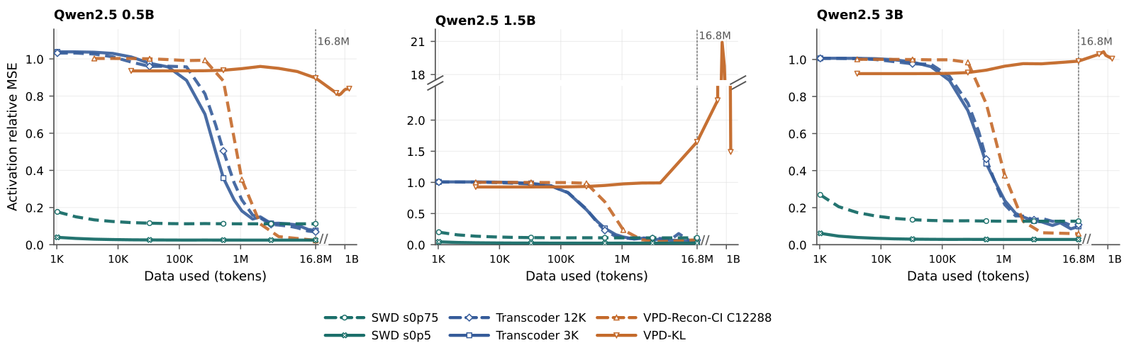
Relative MSE divides aggregated squared projection-output error by aggregated dense-output energy, rather than averaging per-example ratios. KL uses the dense next-token distribution as reference. SWD reaches low error with little calibration data; learned baselines require much more replay. No point on the extended GPT-2 VPD-KL trajectory through 1.6384B tokens satisfies the CE match. Broken logarithmic axes retain the long training tail.
Equations
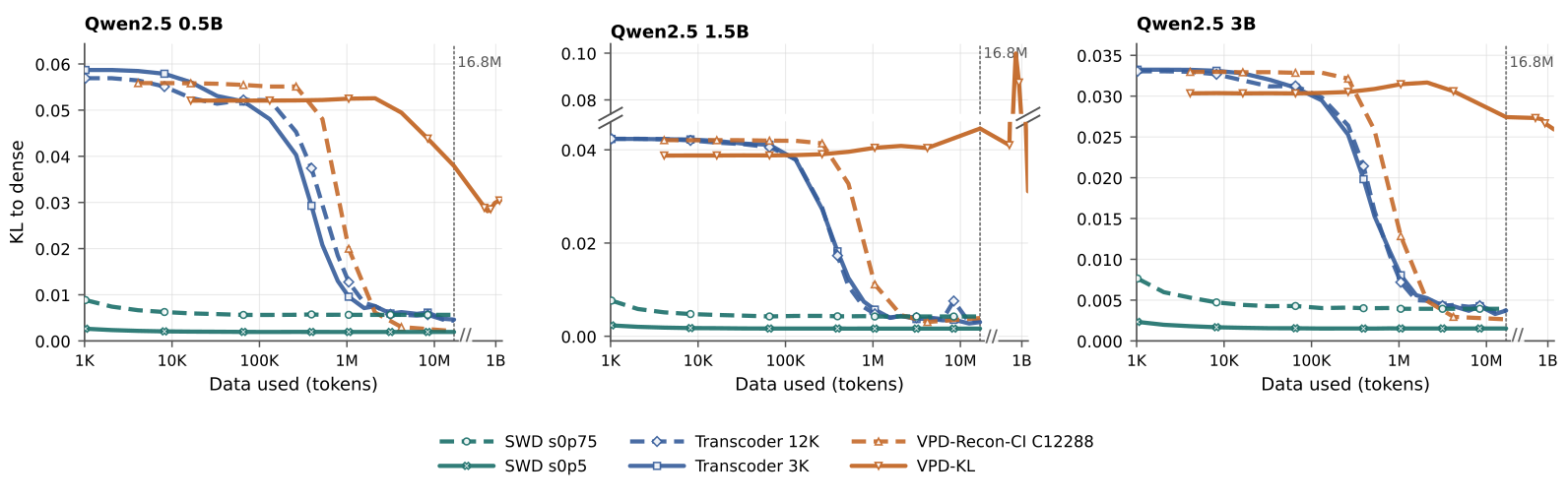
C.2 GPT-2 Selected-Unit Circuit Results
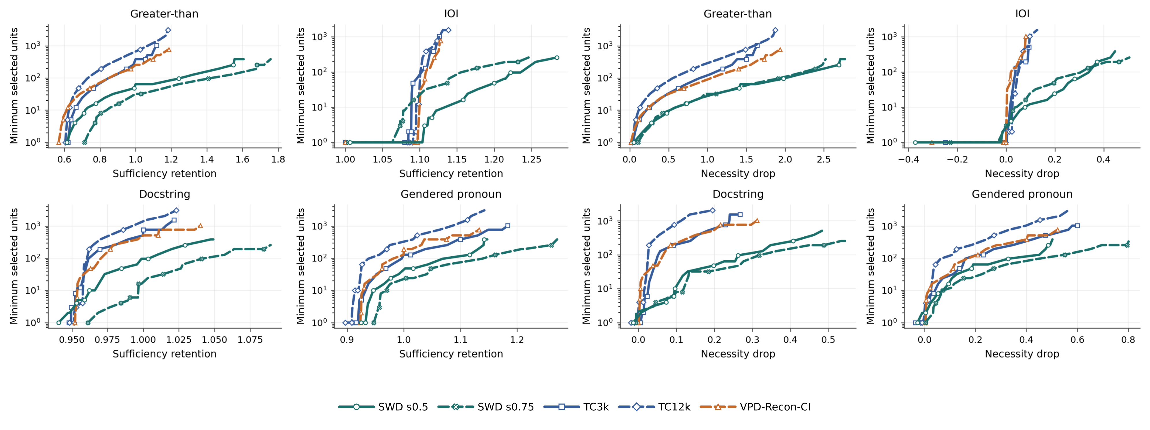
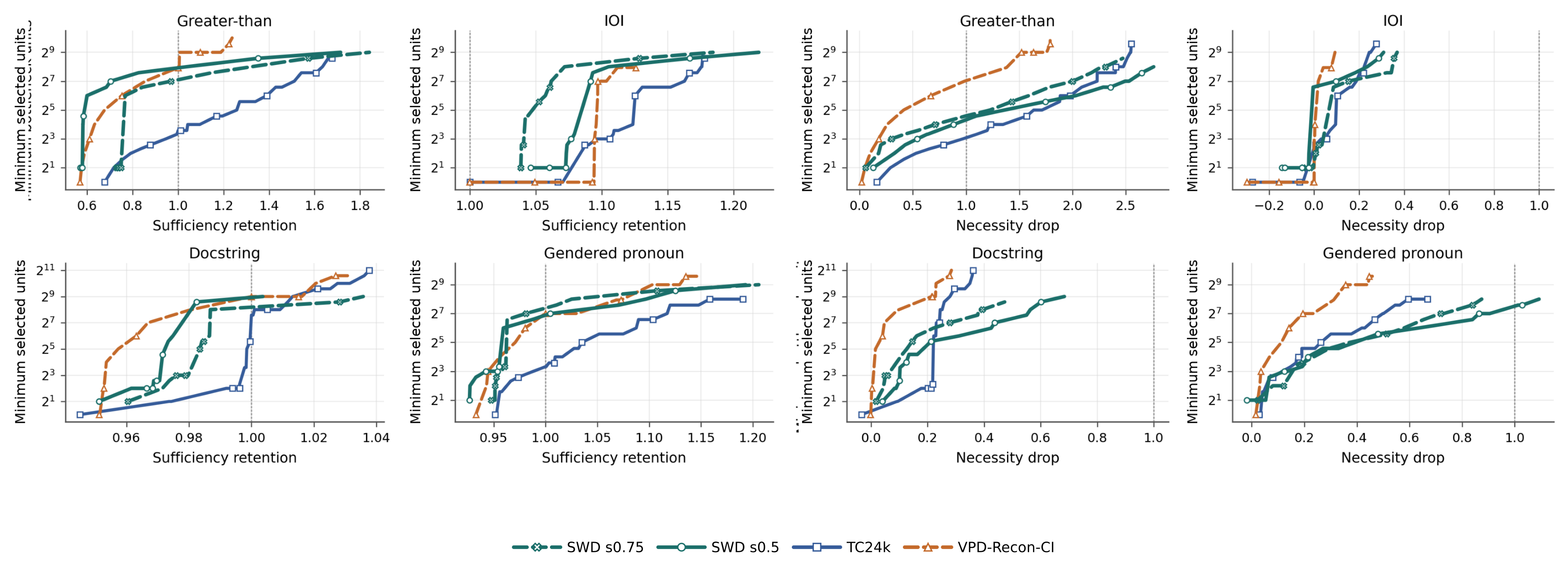
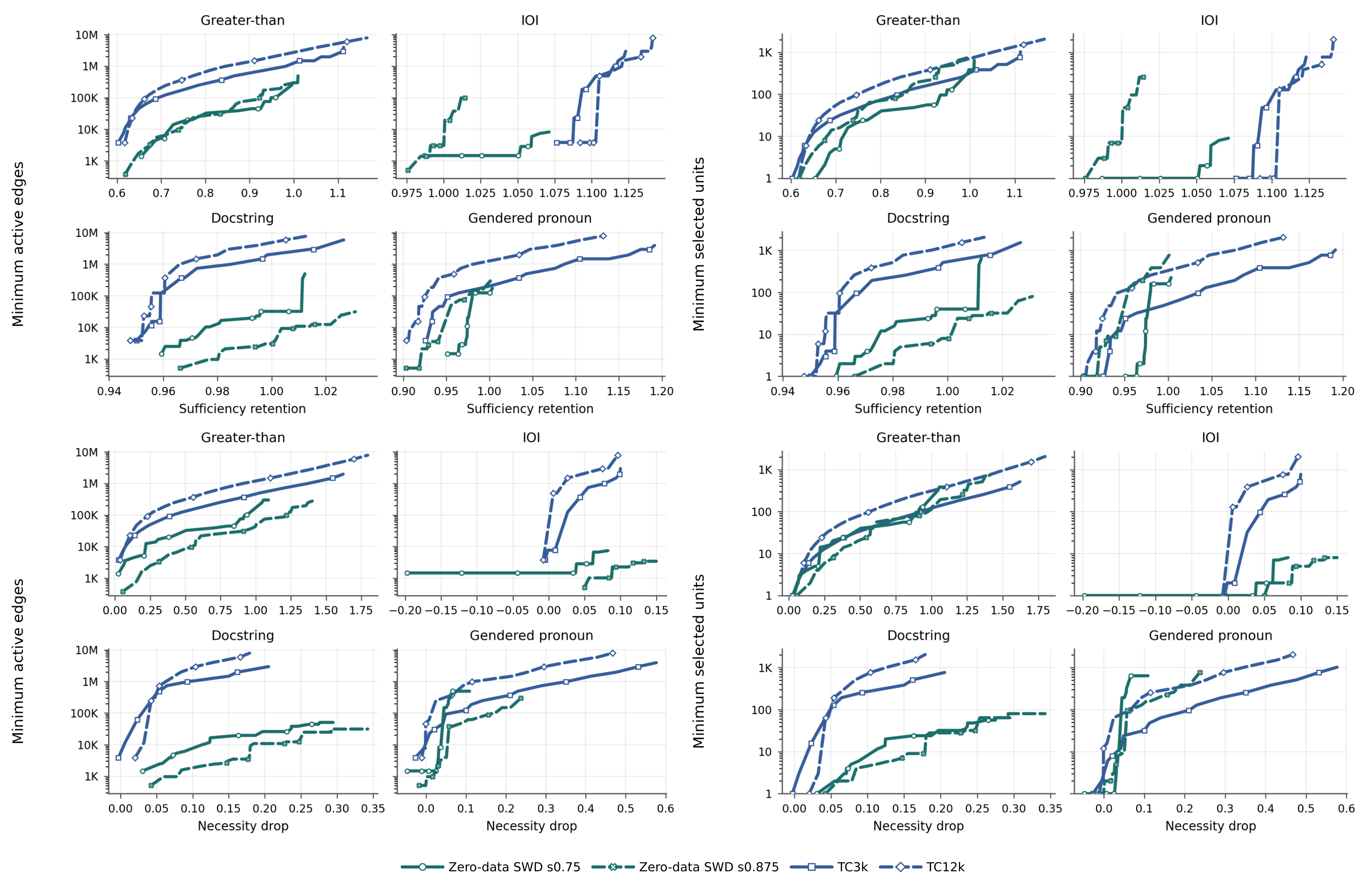
Figure 16 uses selected units for the same GPT-2 output-projection circuits as Figure 3. Sparsity .5, TC3k/TC12k and VPD-Recon-CI form the matched comparison; sparsity .75 remains an explicitly unmatched control.
C.3 Robustness under Zero Ablation
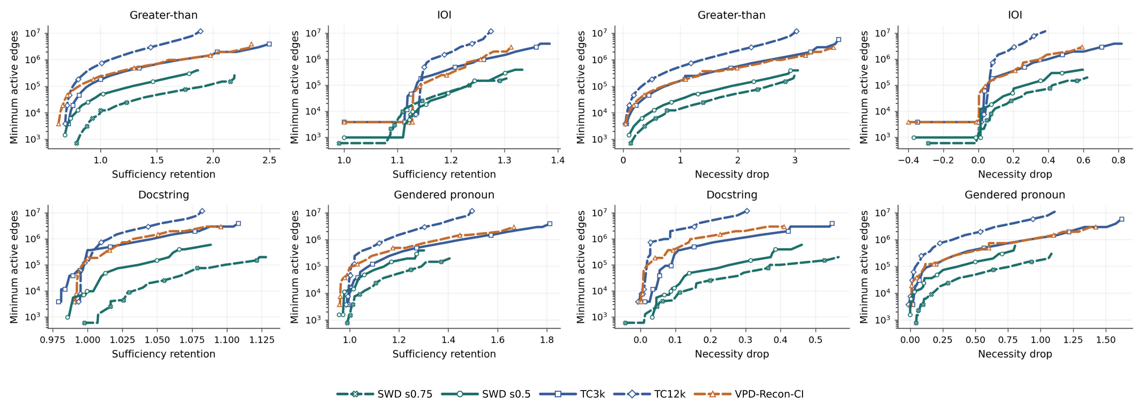
Only the ablated activation value changes from its train mean to zero; checkpoints, scores, rankings, top-k sets and examples stay fixed. SWD’s edge-cost advantage persists on all four GPT-2 tasks. At GreaterThan sufficiency at least one, sparsity .75 uses 12,303 observed edges versus TC3k’s 184,320. This robustness check does not establish invariance to arbitrary intervention protocols.
C.4 Qwen2.5 Circuit Results
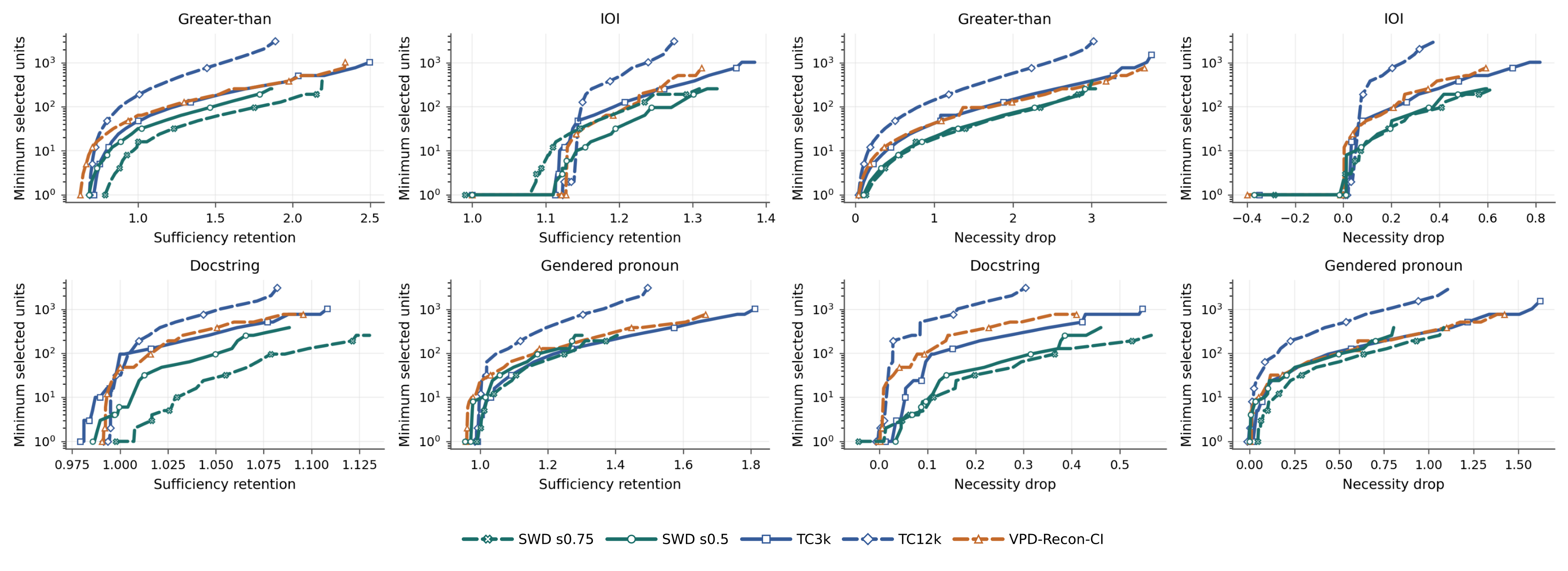
Tables/figures preserve all Qwen2.5 model checkpoints and both cost axes. VPD-Recon-CI uses 12,288 components; VPD-KL appears only in fidelity plots. Unit-count companions separate the number of selected paths from their connectivity.
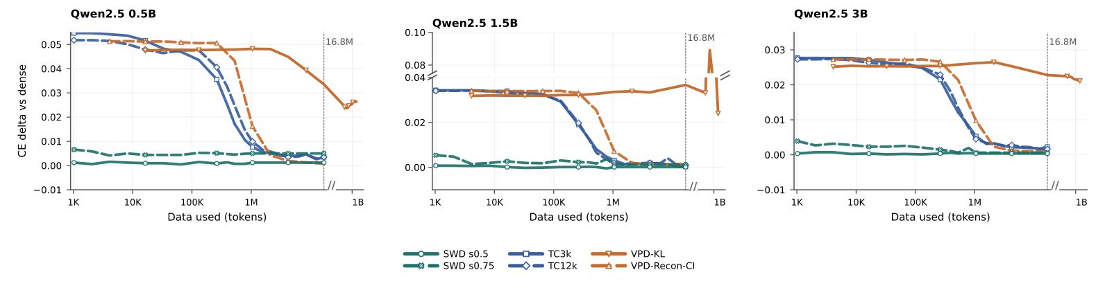
| Model and target module | Checkpoint for circuit extraction | CE delta |
|---|---|---|
| Qwen2.5 0.5B, layer 12 mlp.down_proj | 16.78M tokens used | 0.000729 |
| Qwen2.5 1.5B, layer 14 mlp.down_proj | 4.19M tokens used | 0.001186 |
| Qwen2.5 3B, layer 18 mlp.down_proj | 16.78M tokens used | 0.000906 |
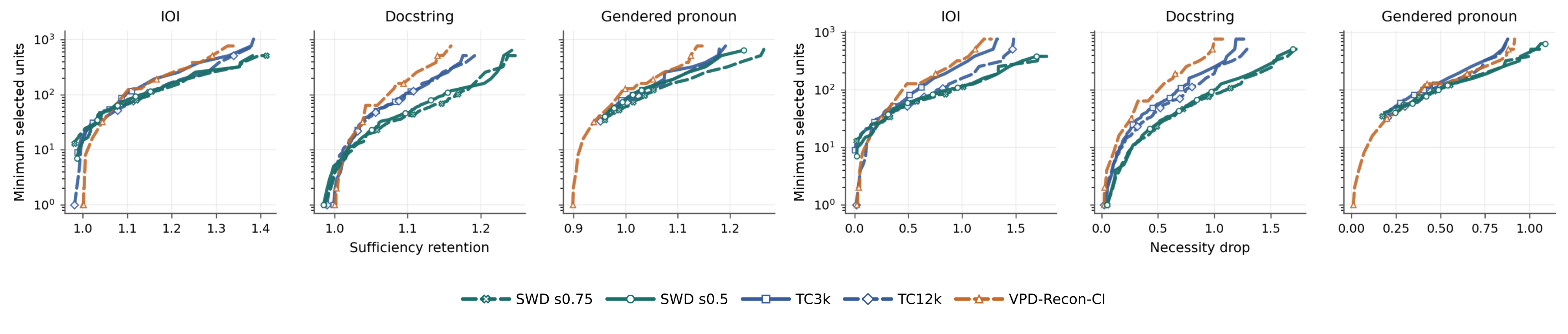
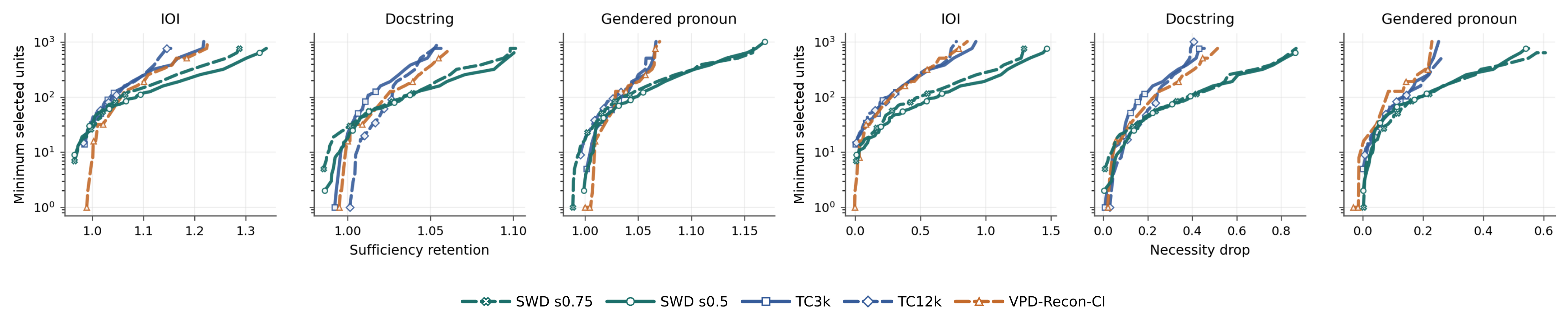
C.5 Qwen3.5-27B Circuit Results
All 27B comparisons use layer-31 down projection and the same three task families. Relative to SWD at sparsity .5, CE differences are .000022 for sparsity .75, .000824 for TC24k, .001121 for TC48k and .002274 for VPD-Recon-CI. Thus the latter two are outside the .001 tolerance, with VPD kept as a contextual reference rather than a fully matched comparison.
| Method | Setting | Checkpoint for circuit extraction | CE delta |
|---|---|---|---|
| SWD | 2,048 calibration tokens | ||
| SWD | 1.05M calibration tokens | ||
| Transcoder | width 24,576 | 134.22M training tokens | |
| Transcoder | width 49,152 | 67.11M training tokens | |
| VPD-Recon-CI | 200.00M training tokens |
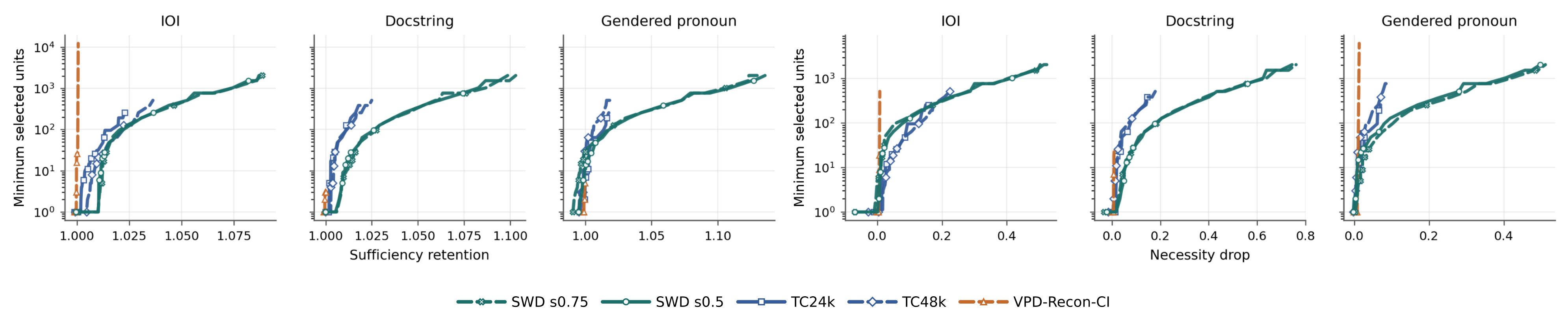
Appendix D Full-Model Replacement
The quality trajectory starts after 4.19M calibration tokens at CE 3.90. Fixed-support finetuning reaches CE 3.44 at 20.6M total presentations, versus sparse pretraining’s 3.45 at 2.884B. Supports remain unchanged throughout SWD finetuning; its curve adds replay tokens to the calibration count.
Appendix E MLP Replacement
Whole-MLP SWD factors both projections while retaining the original intervening GELU and biases. Standard Transcoder replaces the complete input/output map. Quality sweeps share a 16.78M-token horizon, with VPD-KL extended to one billion and still excluded from circuits. The matched circuit checkpoints are SWD .5, TC24k at 6.29M tokens and VPD-Recon-CI at 4.19M. Outcomes are more mixed than single-matrix replacement: SWD is competitive in edge cost and often necessity, while Transcoder is competitive in several sufficiency/unit-count regions.
Equation
| Method | Replacement configuration | Checkpoint for circuit extraction |
|---|---|---|
| SWD | Sequential factorization of c_fc and c_proj; | 16,384 tokens used |
| Transcoder | Standard MLP Transcoder (Appendix B.5.1) | 6.29M tokens used; CE delta 0.003456 |
| VPD-Recon-CI | Local MLP-reconstruction objective; | 4.19M tokens used |
| VPD-KL | Native KL-logit objective; , seed 0 | Replacement only |
Appendix F Exact-Dense Reparameterization Controls
Exact dense controls share the attribution, task data, mean ablation and curve construction with SWD. Their higher active-edge costs cannot be attributed to worse replacement fidelity.
Control configurations.
SVD uses all 768 singular directions of the 3,072×768 target; Random-B uses an orthogonal Gaussian-QR basis with A=WQᵀ. Ten random seeds provide a mean and one-standard-deviation band. Both cost k(3,072+768) edges for k units. SVD CE delta is 1.58×10⁻⁶; Random-B ranges −2.48×10⁻⁶ to 3.40×10⁻⁶. Dense controls can compete in IOI unit count and low docstring necessity, but SWD has the more consistent edge-cost advantage.
Equations
Appendix G Zero-Data Analysis
Weight-only fitting isolates calibration’s contribution while retaining the solver, factor dimensions and budget schedule.
G.1 Factorization and Evaluation Setting
Set the activation Gram matrix to identity and factor GPT-2 layer-8 c_proj across sparsities .125 through .875. Neither supports nor surviving values use calibration activations. Compare each product with calibrated SWD at the same sparsity.
Equation
G.2 Circuit Results
Train-split task data still determines rankings and mean-ablation values; test evaluates the frozen prefixes. At sparsity .375, docstring reaches .962 sufficiency with three units and GreaterThan .986 with 256. Gendered pronouns have fewer strong low-cost outcomes. These results support usable weight-derived paths without claiming calibration-free task evaluation.
Appendix H GreaterThan Case Study: Semantic Audit
The semantic audit ranks all 9,208 valid output-projection units using GreaterThan attribution, then examines independent WikiText-2 activation contexts. GPT-5.5 summarizes recurring patterns in each unit’s twenty strongest passages from 2,048 tokens; these labels do not affect ranking. The six plotted units have global ranks 32–129, with four quantitative and two punctuation/species-name hypotheses. Tables 10–11 preserve ranks and representative contexts. This small model-labeled sample does not establish general monosemanticity.
| Layer | Bottleneck unit | Layer order | Global rank | Score | Semantic hypothesis |
|---|---|---|---|---|---|
| 6 | c380 | 1 | 108 | 10.2 | measure/unit |
| 6 | c723 | 2 | 129 | 9.7 | punctuation/function |
| 6 | c558 | 3 | 152 | 9.3 | mixed lexical |
| 8 | c264 | 1 | 76 | 11.3 | quantity |
| 8 | c511 | 2 | 84 | 11.0 | measure/place |
| 8 | c728 | 3 | 123 | 9.8 | event/time |
| 10 | c757 | 1 | 32 | 14.4 | numeric/year |
| 10 | c627 | 2 | 63 | 11.8 | species/name |
| 10 | c481 | 3 | 85 | 10.9 | numeric/year |
| Bottleneck unit | Semantic hypothesis | Top-activating excerpts |
|---|---|---|
| L6 c380 | measure/unit | “carapace length of 80–85 millimetres”; “usually 23–38 cm”; “a carapace length of 15 mm”. |
| L6 c723 | punctuation/function | Repeated comma-token activations in clauses such as “higher than that of H. americanus, and the European species” and around numeric punctuation. |
| L8 c264 | quantity | “estimated that only 1 larva”; “not normally deeper than 50 m (160 ft)”; “published in 1758”. |
| L8 c511 | measure/place | “48 kilometres or 30 miles northwest of Gothenburg”; “for up to 12 months”; “body length up to 60 centimetres”. |
| L10 c757 | numeric/year | “published in 1758”; “Homarus Weber, 1795”; “Fabricius, 1775”. |
| L10 c627 | species/name | Repeated activations on species-name fragments in “H. americanus”, “H. gammarus”, and “Homarus americanus”. |
Appendix I Targeted Editing of a Single SWD Bottleneck Unit
The editing study follows localized weight-editing and LoRA controls. All methods modify the same original dense layer-8 matrix, avoiding replacement-fidelity confounds. A sparsity-.75 factorization fitted on 131,072 WikiText-2 tokens supplies c205’s read vector; a rank-one write update is calibrated to a requested local answer-direction shift. The unit/target were screened from eight triples and top-24 candidate units. Random c540 is sampled from a middle activation range; the dense oracle directly uses the target activation. Rank-4 LoRA trains separately for each requested margin shift for 180 AdamW steps. At local shift three, the realized final margin changes only .215797; seven non-target prompts give KL 4.02375×10⁻⁵ and a separate 504-token sample 1.96415×10⁻⁵. The oracle is strongest; c205 improves the measured tradeoff over random/LoRA on this selected case.
Equations
Appendix J Attention Bottleneck Units: From Static QK Geometry to Prompt-Local Effects
Attention analysis combines QK-circuit geometry, sparse weight-space decomposition and feature-level attribution. It first checks reconstruction, then screens static pairs and tests prompt-specific contributions causally.
J.1 Attention Factorization Fidelity
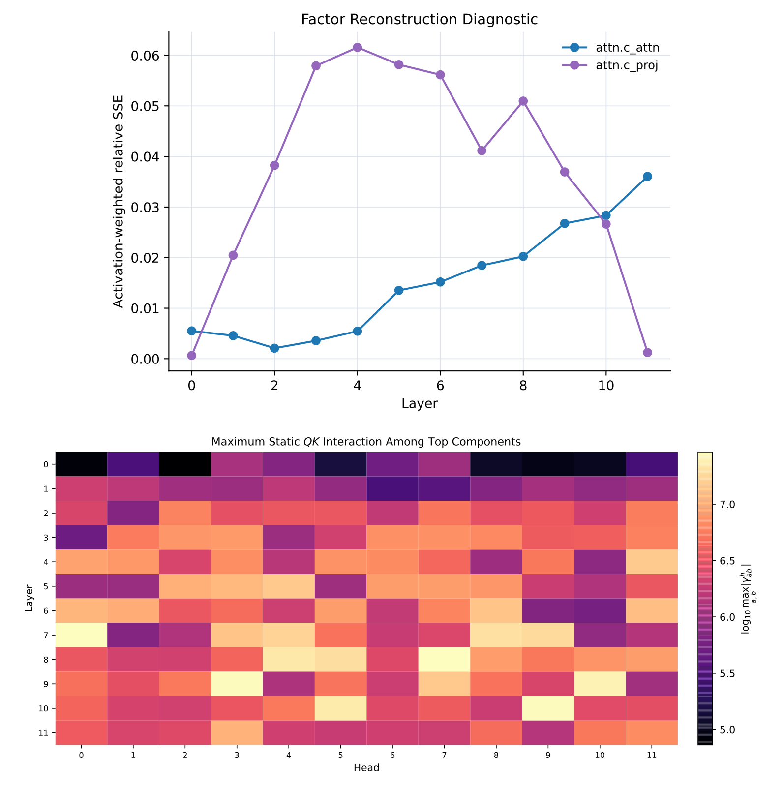
Across GPT-2’s twelve layers, packed Q/K/V reconstruction relative SSE stays below four percent. Attention output-projection error reaches roughly six percent in middle layers. The replay case therefore uses the better-preserved Q/K/V factors and independently verifies its attention pattern.
J.2 Static QK Candidate Screen
A head’s bilinear query/key score expands into pair contributions: activation product times a static write-direction inner product scaled by √64. In each of 144 layer/head combinations, retain sixteen largest-norm query and key units, inspect all 256 pairs, and advance the five largest static interactions to prompt replay. Static geometry alone does not establish a contribution on a particular input.
Equations
J.3 Prompt Replay and Bottleneck-Unit Intervention
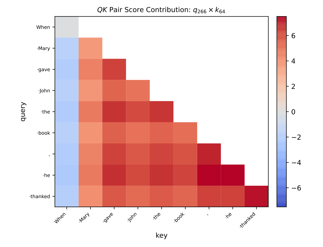
Five pairs per layer/head on three prompts yield 2,160 evaluations. The selected q266×k64 case is layer 9/head 3 on “When Mary gave John the book, he thanked”. Reconstructed attention has dense-reference KL .0405; the pair’s signed mean contribution is +4.26, suppressing the first key while favoring later keys. Removing q266 from the reconstructed query slice redirects attention to the first token, with KL 2.496 and maximum change .775. This verifies one selected prompt-local effect, not all attention units.
Equations
Appendix K Interaction Patterns among MLP Bottleneck Units
The diagnostics distinguish correlation of additive post-GELU output paths from contextual non-additivity of pre-GELU input paths. Superposition and nonlinear interactions motivate checking combinations rather than assuming independent units.
K.1 c_proj : Linear Contributions Are Usually Weakly Correlated
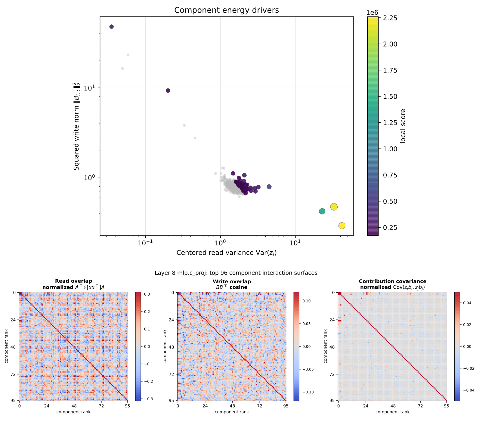
For 768 layer-8 c_proj units at sparsity .75, 2,048 held-out tokens estimate read correlations, write-direction cosines and full residual-contribution correlations. The 96 highest-energy units appear in matrix views; distributions cover all units. The respective 95th-percentile magnitudes are .207, .071 and .0049, so overlapping reads/writes rarely coincide strongly. A small tail recurs around c373/c447/c481/c266; c373–c481 reaches .345 because opposed reads and opposed writes cancel their signs.
Equation
K.2 c_fc and GELU: Contextual Pair Interactions
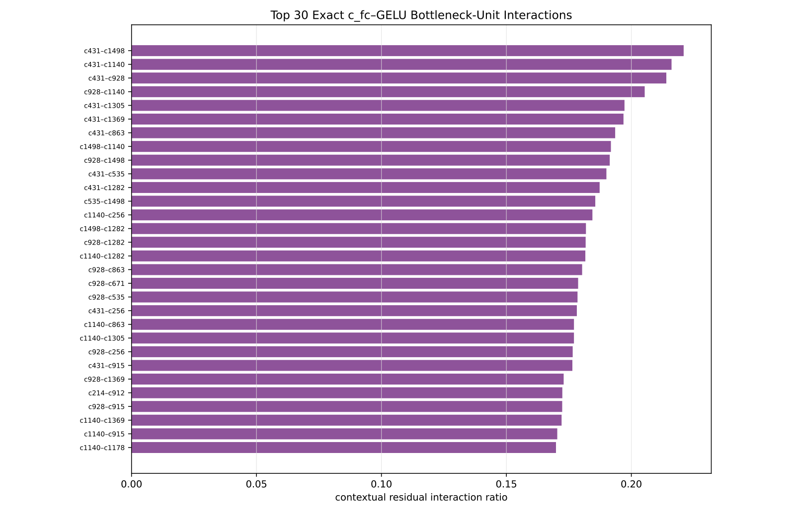
The c_fc diagnostic replays 8,192 held-out tokens with lower-layer replacements installed. Select 128 high-energy paths from 1,536 units, yielding 8,128 pairs. A contextual second finite difference across GELU is projected through the original output matrix and normalized by individual marginal residual energies. Interaction ratios average .093, median .089, 95th percentile .132 and maximum .221; 2,130 pairs are at least .10. Recurring high-energy units and isolated strong pairs form a moderate interaction field, contrasting with mostly weak output-path correlation.
Equations