Overview
The paper studies dense monocular simultaneous localization and mapping over long trajectories.
At a glance
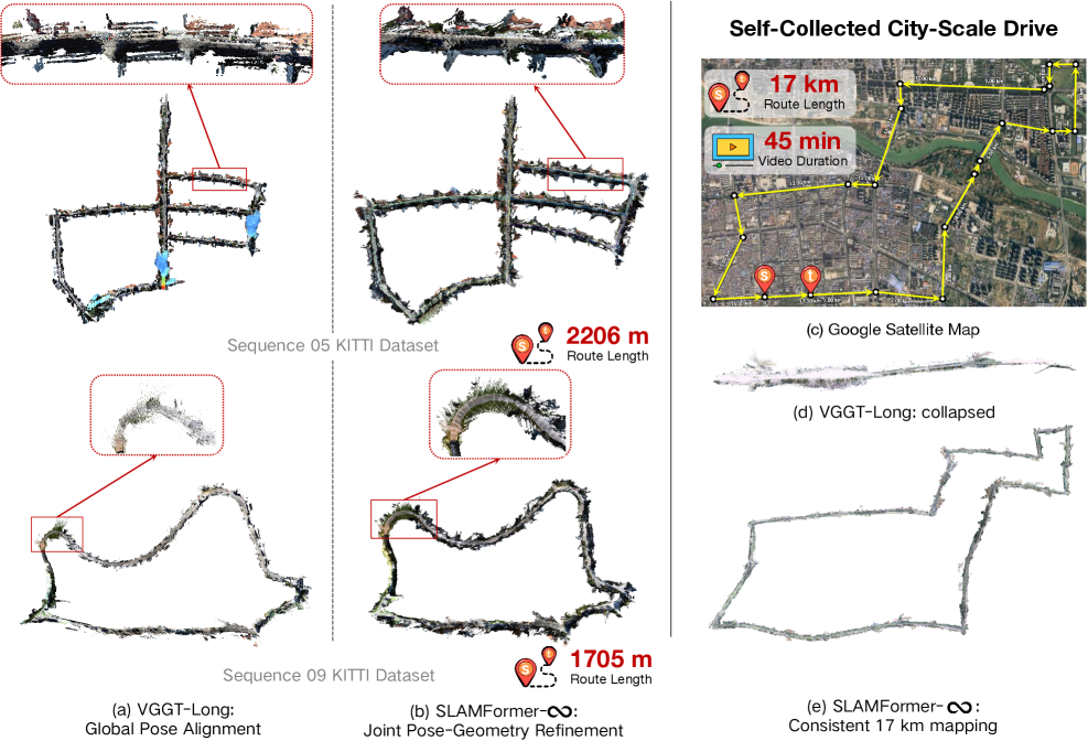
SLAMFormer-∞ conditions a geometric transformer on memory frames and poses to define local coordinates. A bounded local frontend tracks incoming frames, while an iterative graph-based backend jointly refines poses and dense pointmaps. The method improves several long outdoor benchmarks and demonstrates a self-collected drive exceeding 17 km. “Infinite” denotes removal of a fixed inference-distance formulation, not a guarantee of unlimited accuracy, runtime, or memory.
1 Introduction
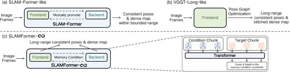
Earlier transformer systems either depend on a training-scale global coordinate system or correct poses while leaving much local geometry fixed. This method uses persistent local geometric anchors and applies the same transformer to graph neighborhoods during global refinement. The contribution is a conditioned representation and pose–geometry graph optimization, with stronger long-range reconstruction in the reported tests. The graph and stored map still grow with the explored environment.
2 Related Work
The comparison spans feedforward geometric transformers and learned SLAM pipelines.
2.1 Geometric Transformer
Pairwise and multiview geometric models predict pointmaps and camera relations, but finite attention context and coordinate conventions complicate long trajectories. Recurrent states and chunk alignment extend their range. SLAMFormer-∞ instead uses conditioned local references so distant information can enter iterative refinement through graph connections.
2.2 Learning-based SLAM
Prior dense SLAM combines learned matching, rendering losses, submaps, or pose optimization. SLAM-Former moves frontend and backend inference into one transformer, but its history representation grows. The new method replaces full-history refinement with repeated local pose–geometry graph updates. It still depends on external graph construction and, outdoors, pose-graph initialization.
3 Methodology
The method defines local conditional inference, joint graph refinement, test-time scheduling, and four shared-weight training modes.
3.1 Problem Formulation
Given a monocular RGB stream, the system estimates camera poses and per-frame pointmaps. The previous SLAM-Former formulation maintains map tokens: a causal frontend updates them and a backend refines the accumulated history. Prediction heads decode poses and geometry. The preserved frontend/backend equations specify the original causal and whole-history prediction functions.
Equations


3.2 SLAMFormer- ∞
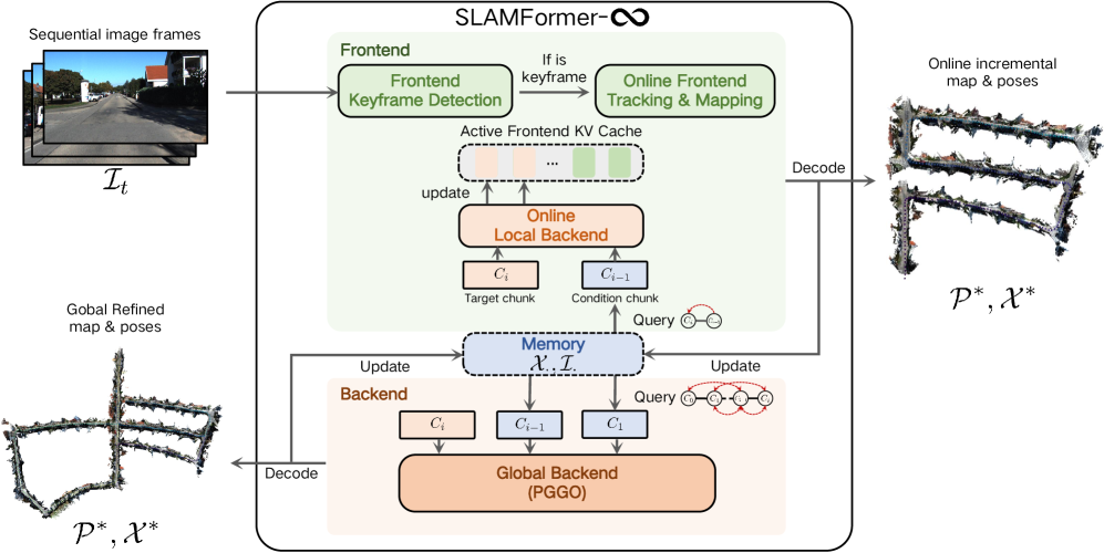
Memory images and poses define the reference frame for a local prediction window. The frontend uses cached keys and values from nearby frames and anchors; the backend refines a local target span conditioned on neighboring context. This relative formulation permits bounded attention neighborhoods, but global consistency requires repeated graph updates rather than one full-history attention pass.
Equations


3.3 Pose-Geometry Graph Optimization (PGGO)
Each graph state combines a camera pose and dense pointmap. Explicit pose edges and transformer-mediated geometry relations connect states. Starting from frontend or pose-graph estimates, the model predicts revised states repeatedly. Pointmaps are replaced directly, while poses receive damped updates using logarithm and exponential maps. The preserved objective and update equations describe a learned refinement scheme; the paper does not prove convergence or global optimality for arbitrary graphs.
Equations 5
| (5) |
Equation

3.4 SLAM at Test Time
Incoming frames are associated with existing keyframes or create new graph nodes. A local backend runs after a fixed number of keyframes. Loop detections or sequence completion trigger global pose–geometry refinement over graph neighborhoods. These stages distinguish streaming tracking from later global processing; a long-sequence reconstruction result does not alone establish that every global update is real time.
3.5 Training Strategy
Four attention/conditioning modes share model weights. The frontend mode begins with two mutually attending frames and then uses causal attention. An unconditioned backend refines a prefix before causal decoding. A conditioned backend uses detached prefix predictions aligned to an anchor. The fine-stage mode conditions a middle target chunk on both preceding and following chunks, matching bidirectional graph refinement at test time.
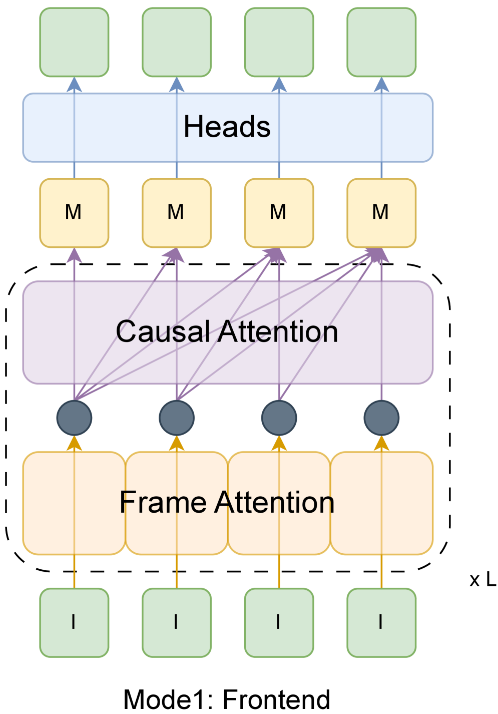
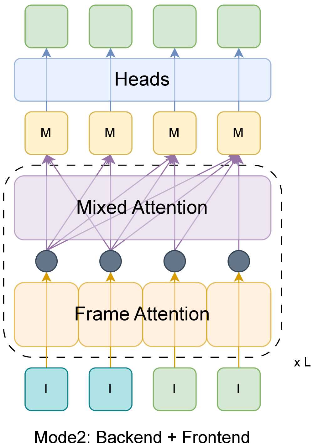
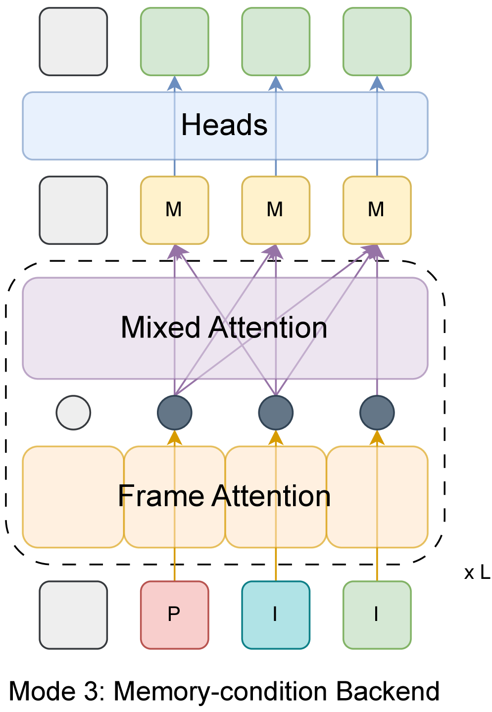
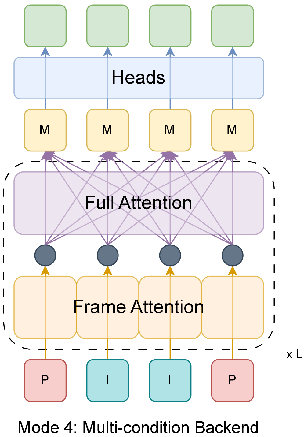
 and
 represent the image tokens fed into the frontend and backend.
 represents the image tokens injected with pose.
 represents the map tokens of a frame.
 and
 represent the layer intermediate and final output.
In each mode,
,
and
are fed into the transformer backbone , with layers of frame attention and various inter-frame attentions.
Pose and pointmap are regressed by the heads .
4 Experiments
Evaluation separates large outdoor trajectories, shorter indoor scenes, and the effect of the final refinement stage.
4.1 Experimental Setup
Indoor and outdoor variants use distinct training scales. Tracking and dense geometry are evaluated separately, and baseline calibration requirements are retained in the tables.
Training setup.
Both variants initialize from pretrained SLAM-Former and train for ten epochs on 48 A100 GPUs. Indoor clips have 12 frames at long-side resolution 518; outdoor clips have 36 frames at 224. Dataset mixtures and optimization settings are retained in Appendix A.
Evaluation protocol.
Indoor tests use Replica, TUM RGB-D, and 7-Scenes; outdoor tests use KITTI and nine Waymo segments. Absolute trajectory error is reported as root-mean-square error in meters. Reconstruction uses accuracy, completeness, and Chamfer distance, all lower-is-better. Some baselines receive camera calibration while calibration-free methods do not. Out-of-memory and tracking-loss entries are failures under the stated setup, not finite scores.
4.2 Large Outdoor Scenes
Outdoor refinement starts from pose-graph optimization configured consistently with VGGT-Long. Its gains therefore reflect learned pose–geometry refinement on top of that initialization, not removal of all conventional optimization.
Tracking performance.
Mean KITTI trajectory error falls from VGGT-Long’s 26.358 m to 23.011 m; Waymo falls from 1.996 m to 1.813 m. Improvements are not uniform across sequences. KITTI’s calibrated LDSO baseline has a slightly lower full-sequence mean, and excluding the high-speed sequence changes the ranking. The strongest claim is competitive long-range tracking combined with dense calibration-free reconstruction.
| Method | LC | Calibration | Recon. | Avg. | Avg.∗ | 00 | 01 | 02 | 03 | 04 | 05 | 06 | 07 | 08 | 09 | 10 | |
| seq. frames | - | - | - | 2109 | 2210 | 4542 | 1101 | 4661 | 801 | 271 | 2761 | 1101 | 1101 | 4071 | 1591 | 1201 | |
| seq. length (m) | - | - | - | 2012.243 | 1968.147 | 3724.19 | 2453.20 | 5067.23 | 560.89 | 393.65 | 2205.58 | 1232.88 | 649.70 | 3222.80 | 1705.05 | 919.52 | |
| seq. speed (m / frame) | - | - | - | 0.95 | 0.89 | 0.82 | 2.23 | 1.09 | 0.70 | 1.45 | 0.80 | 1.12 | 0.59 | 0.79 | 1.07 | 0.77 | |
| contains loop | - | - | - | - | - | ✓ | ✗ | ✓ | ✗ | ✗ | ✓ | ✓ | ✓ | ✗ | ✓ | ✗ | |
| Classic | ORB-SLAM2 [21] (w/o LC) | ✗ | Required | Sparse | 69.727 | 26.480 | 40.65 | 502.20 | 47.82 | 0.94 | 1.30 | 29.95 | 40.82 | 16.04 | 43.09 | 38.77 | 5.42 |
| ORB-SLAM2[21] (w/ LC) | ✓ | Required | Sparse | 54.816 | 9.464 | 6.03 | 508.34 | 14.76 | 1.02 | 1.57 | 4.04 | 11.16 | 2.19 | 38.85 | 8.39 | 6.63 | |
| LDSO [10] | ✓ | Required | Sparse | 22.425 | 23.500 | 9.32 | 11.68 | 31.98 | 2.85 | 1.22 | 5.10 | 13.55 | 2.96 | 129.02 | 21.64 | 17.36 | |
| Learning Based | DROID-VO [27] | ✗ | Required | Dense | 54.188 | 51.187 | 98.43 | 84.20 | 108.80 | 2.58 | 0.93 | 59.27 | 64.40 | 24.20 | 64.55 | 71.80 | 16.91 |
| DPVO [28] | ✗ | Required | Sparse | 53.609 | 57.701 | 113.21 | 12.69 | 123.40 | 2.09 | 0.68 | 58.96 | 54.78 | 19.26 | 115.90 | 75.10 | 13.63 | |
| DROID-SLAM [27] | - | Required | Dense | 100.278 | 75.846 | 92.10 | 344.60 | 107.61 | 2.38 | 1.00 | 118.50 | 62.47 | 21.78 | 161.60 | 72.32 | 118.70 | |
| DPV-SLAM [17] | ✓ | Required | Sparse | 53.034 | 57.187 | 112.80 | 11.50 | 123.53 | 2.50 | 0.81 | 57.80 | 54.86 | 18.77 | 110.49 | 76.66 | 13.65 | |
| DPV-SLAM++ [17] | ✓ | Required | Sparse | 25.749 | 27.138 | 8.30 | 11.86 | 39.64 | 2.50 | 0.78 | 5.74 | 11.60 | 1.52 | 110.90 | 76.70 | 13.70 | |
| MASt3R-SLAM [22] | ✓ | No Need | Dense | / | / | TL | TL | TL | TL | TL | TL | TL | TL | TL | TL | TL | |
| CUT3R [31] | ✗ | No Need | Dense | / | / | OOM | OOM | OOM | 148.07 | 22.31 | OOM | OOM | OOM | OOM | OOM | OOM | |
| Fast3R [35] | ✗ | No Need | Dense | / | / | OOM | OOM | OOM | OOM | OOM | OOM | OOM | OOM | OOM | OOM | OOM | |
| VGGT [30] | ✗ | No Need | Dense | / | / | OOM | OOM | OOM | OOM | OOM | OOM | OOM | OOM | OOM | OOM | OOM | |
| VGGT-Long [8] | ✓ | No Need | Dense | 26.358 | 19.298 | 8.06 | 96.96 | 34.16 | 6.83 | 4.16 | 9.15 | 4.68 | 2.68 | 63.15 | 32.24 | 27.87 | |
| SLAMFormer- | ✓ | No Need | Dense | 23.011 | 15.653 | 15.39 | 96.58 | 28.81 | 4.97 | 4.16 | 11.36 | 13.54 | 8.53 | 37.00 | 18.85 | 13.93 |
| Segment ID | Calib. | Avg. | 163453191 | 183829460 | 315615587 | 346181117 | 371159869 | 405841035 | 460417311 | 520018670 | 610454533 |
| Frame num. | - | 198 | 198 | 199 | 199 | 199 | 196 | 199 | 198 | 199 | 198 |
| Segment length | - | 172.533 | 159.963 | 42.301 | 165.149 | 351.213 | 272.661 | 85.743 | 265.906 | 134.552 | 62.739 |
| Segment speed | - | 0.871 | 0.808 | 0.213 | 0.830 | 1.765 | 1.391 | 0.431 | 1.343 | 0.676 | 0.317 |
| Traffic | - | - | Low | High | Low | Low | Medium | Low | Medium | Low | High |
| DROID-SLAM [27] | Required | 4.396 | 3.705 | 0.301 | 0.447 | 8.653 | 9.320 | 7.621 | 4.170 | TL | 0.264 |
| MASt3R-SLAM [22] | No Need | 5.560 | 4.500 | 0.556 | 1.833 | 12.544 | 8.601 | 1.412 | 5.428 | 7.910 | 1.195 |
| CUT3R [31] | No Need | 9.872 | 8.781 | 3.810 | 5.790 | 24.015 | 13.070 | 7.261 | 13.206 | 8.597 | 3.229 |
| Fast3R [35] | No Need | / | OOM | OOM | OOM | OOM | OOM | OOM | OOM | OOM | OOM |
| VGGT [30] | No Need | / | OOM | OOM | OOM | OOM | OOM | OOM | OOM | OOM | OOM |
| VGGT-Long [8] | No Need | 1.996 | 1.753 | 2.629 | 0.559 | 3.452 | 3.343 | 1.444 | 1.541 | 2.547 | 0.455 |
| SLAMFormer- | No Need | 1.813 | 1.270 | 0.616 | 0.810 | 1.464 | 5.281 | 0.568 | 3.116 | 2.825 | 0.371 |
Reconstruction performance.
On Waymo, average pointmap accuracy/completeness/Chamfer scores change from 1.182/2.860/2.021 to 0.949/2.777/1.863. Figures show more coherent local surfaces than pose-aligned stitching on selected KITTI sequences. The opening figure also depicts a self-collected 17 km drive, providing a long-range demonstration rather than a broad statistical benchmark of that distance.
| Segment ID | Metric | Calib. | Avg. | 163453191 | 183829460 | 315615587 | 346181117 | 371159869 | 405841035 | 460417311 | 520018670 | 610454533 |
|---|---|---|---|---|---|---|---|---|---|---|---|---|
| Frame num. | - | - | 198 | 198 | 199 | 199 | 199 | 196 | 199 | 198 | 199 | 198 |
| Segment length | - | - | 172.533 | 159.963 | 42.301 | 165.149 | 351.213 | 272.661 | 85.743 | 265.906 | 134.552 | 62.739 |
| Segment speed | - | - | 0.871 | 0.808 | 0.213 | 0.830 | 1.765 | 1.391 | 0.431 | 1.343 | 0.676 | 0.317 |
| Traffic | - | - | - | Low | High | Low | Low | Medium | Low | Medium | Low | High |
| DROID-SLAM [27] | Accuracy | Required | 1.201 | 0.781 | 1.136 | 2.247 | 2.393 | 1.090 | 0.539 | 0.740 | TL | 0.677 |
| Completeness | 8.540 | 4.610 | 10.245 | 5.540 | 8.669 | 8.592 | 11.144 | 5.320 | TL | 14.201 | ||
| Chamfer | 4.870 | 2.696 | 5.691 | 3.893 | 5.531 | 4.841 | 5.842 | 3.030 | TL | 7.439 | ||
| MASt3R-SLAM [22] | Accuracy | No Need | 3.772 | 3.189 | 2.988 | 3.787 | 4.689 | 4.436 | 1.166 | 4.637 | 6.417 | 2.637 |
| Completeness | 3.177 | 1.715 | 3.284 | 2.047 | 2.981 | 2.679 | 2.895 | 2.002 | 4.429 | 6.560 | ||
| Chamfer | 3.474 | 2.452 | 3.136 | 2.917 | 3.835 | 3.558 | 2.031 | 3.319 | 5.423 | 4.599 | ||
| CUT3R [31] | Accuracy | No Need | 3.884 | 3.580 | 1.144 | 2.418 | 3.712 | 3.679 | 4.346 | 2.012 | 12.320 | 1.744 |
| Completeness | 6.801 | 8.251 | 9.352 | 8.748 | 8.537 | 5.467 | 3.393 | 6.164 | 2.302 | 8.999 | ||
| Chamfer | 5.343 | 5.916 | 5.248 | 5.583 | 6.125 | 4.573 | 3.869 | 4.088 | 7.311 | 5.371 | ||
| VGGT-Long [8] | Accuracy | No Need | 1.182 | 1.002 | 0.395 | 0.925 | 1.668 | 2.580 | 0.679 | 0.784 | 1.358 | 1.246 |
| Completeness | 2.860 | 2.762 | 3.417 | 1.738 | 3.261 | 2.791 | 3.216 | 1.840 | 4.694 | 2.022 | ||
| Chamfer | 2.021 | 1.882 | 1.906 | 1.331 | 2.465 | 2.685 | 1.948 | 1.312 | 3.026 | 1.634 | ||
| SLAMFormer- | Accuracy | No Need | 0.949 | 0.601 | 0.467 | 1.454 | 1.064 | 1.964 | 0.251 | 1.268 | 0.935 | 0.540 |
| Completeness | 2.777 | 2.562 | 3.191 | 1.965 | 2.815 | 3.259 | 5.461 | 2.174 | 1.025 | 2.538 | ||
| Chamfer | 1.863 | 1.582 | 1.829 | 1.709 | 1.939 | 2.611 | 2.856 | 1.721 | 0.980 | 1.539 |
4.3 Small Indoor Scenes
On 7-Scenes, trajectory error improves over VGGT-SLAM from 0.068 m to 0.046 m and Chamfer distance from 0.057 to 0.039. Indoor performance remains below the original SLAM-Former in the reported aggregate table. Matching-based methods are also stronger on parts of Replica. The design prioritizes long-range refinement and does not dominate every shorter-scene metric.
| Method | TUM RGB-D | 7-Scenes | Replica | |||||
|---|---|---|---|---|---|---|---|---|
| ATE | ATE | Acc. | Comp. | Chamf. | ATE | Acc. | Comp. | |
| CUT3R [31] | 0.113 | 0.073 | 0.032 | 0.047 | 0.040 | 0.170 | 7.52 | 3.62 |
| StreamVGGT [41] | 0.187 | 0.081 | 0.058 | 0.057 | 0.057 | 0.125 | 9.88 | 4.73 |
| VGGT-SLAM [19] | 0.084 | 0.068 | 0.054 | 0.060 | 0.057 | 0.071 | 7.52 | 5.86 |
| MASt3R-SLAM [22] | 0.061 | 0.065 | 0.065 | 0.067 | 0.056 | 0.045 | 2.92 | 2.25 |
| EC3R-SLAM [13] | 0.070 | 0.075 | 0.025 | 0.054 | 0.040 | 0.041 | 2.82 | 2.07 |
| VGGT-Long [8]+ | 0.082 | 0.089 | 0.049 | 0.081 | 0.065 | 0.071 | 5.80 | 3.17 |
| SLAM-Former [39] | 0.039 | 0.042 | 0.017 | 0.037 | 0.027 | 0.030 | 2.09 | 1.56 |
| SLAMFormer- | 0.066 | 0.046 | 0.029 | 0.049 | 0.039 | 0.052 | 6.00 | 3.33 |
| SLAMFormer- (w/o fine) | 0.068 | 0.047 | 0.030 | 0.049 | 0.040 | 0.061 | 6.11 | 3.39 |
4.4 Ablation Study: Before and After Fine Stage (PGGO)
The fine stage yields modest numeric improvements: Replica trajectory error decreases from 0.061 m to 0.052 m, with the table’s accuracy/completeness values changing from 6.11/3.39 to 6.00/3.33. Improvements on TUM and 7-Scenes are smaller. Retained visual comparisons show cleaner surfaces. Units for the reconstruction columns are not specified consistently enough to equate their scale with trajectory meters.

5 Limitations
Graph connectivity comes from the frontend and loop detection rather than being learned end to end. Poor or missing connections can therefore limit refinement. Local attention removes one scale restriction, but the experiments do not establish arbitrary-distance robustness or a global consistency guarantee.
6 Conclusion
Conditioned local coordinates and iterative joint pose–geometry refinement improve long-range reconstruction while maintaining competitive localization. The 17 km demonstration illustrates the intended operating regime; indoor results and graph dependence remain material limitations.
Appendix A Training Details
The indoor mix combines ARKitScenes, ScanNet++, ScanNet, HyperSim, BlendedMVS, and MegaDepth. The outdoor mix adds VirtualKITTI2, TartanGround, and HabitatHM3D while retaining several shared datasets. Both configurations use batch size one per GPU, no gradient accumulation, AdamW weight decay 0.05, a cosine schedule from 10⁻⁵ to 10⁻⁸, half an epoch of warm-up, and mixed precision. Training takes roughly one hour per indoor epoch and 2.5 hours per outdoor epoch on 48 A100 GPUs.
| Configuration | Datasets | Clip length | Long side |
|---|---|---|---|
| Indoor | ARKitScenes [1], ScanNet++ [37], ScanNet [6], HyperSim [24], BlendedMVS [36], MegaDepth [16] | 12 | 518 |
| Outdoor | VirtualKITTI2 [2], TartanGround [23], HabitatHM3D [34], ARKitScenes [1], ScanNet++ [37], BlendedMVS [36], MegaDepth [16] | 36 | 224 |
| Hyperparameter | Value |
|---|---|
| Batch size | 1 per GPU |
| Gradient accumulation | None |
| Optimizer | AdamW |
| Weight decay | 0.05 |
| Initial learning rate | |
| Minimum learning rate | |
| LR schedule | Cosine decay |
| Warm-up | 0.5 epochs |
| Precision | Mixed precision |
| Training epochs | 10 |
| GPUs | 48 A100 |
| Indoor training time | 1 hour / epoch |
| Outdoor training time | 2.5 hours / epoch |
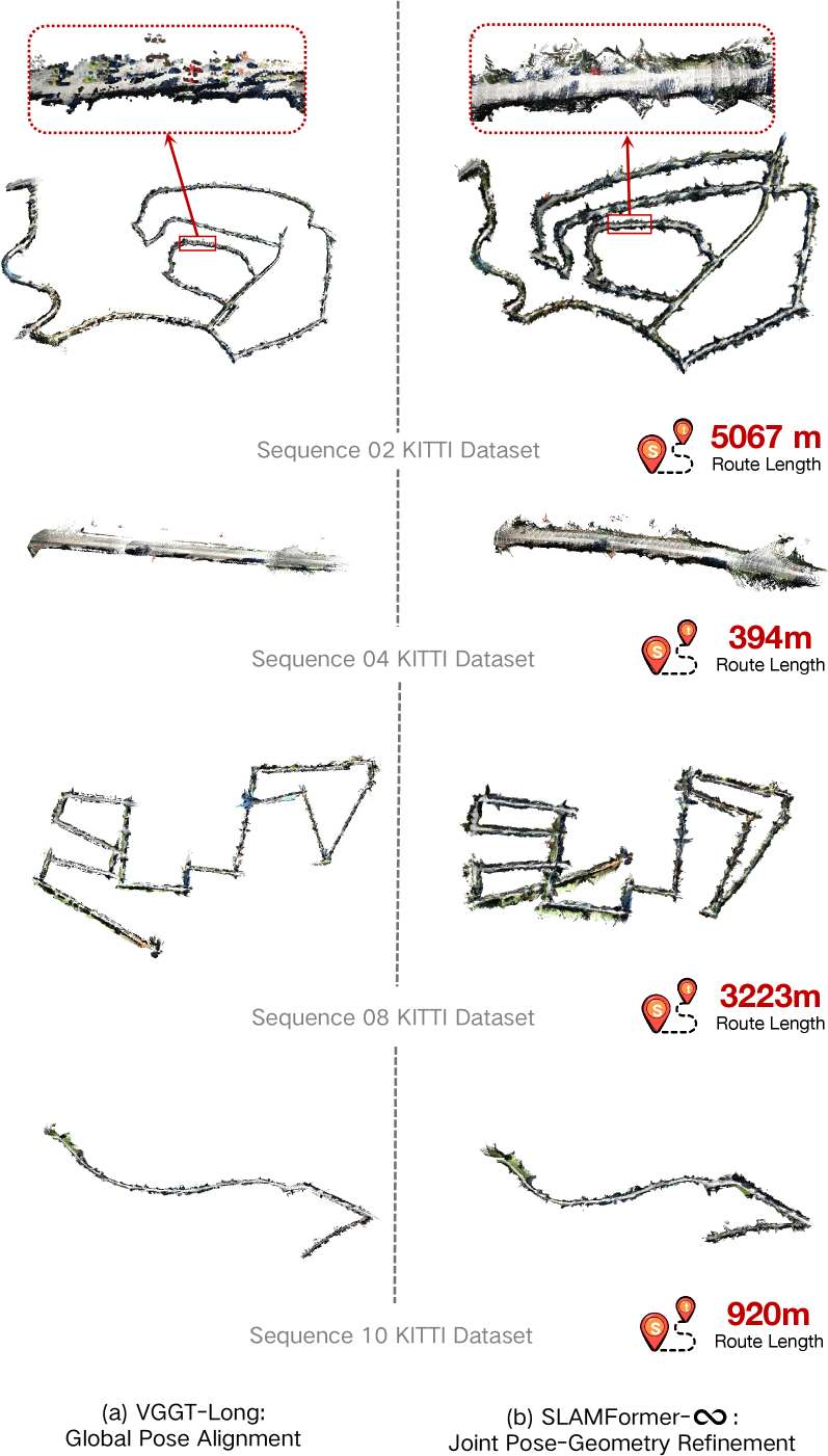
Appendix B Qualitative Analysis on KITTI
Additional KITTI views compare pose-aligned stitched maps with joint refinement. The zooms illustrate fragmented or misaligned local surfaces in the baseline and more coherent geometry in the proposed method. They supplement the benchmark scores but do not independently quantify every visual difference.