Literature
Display
← All papers

Self-supervised DXA representations encode multi-system disease risk, biological aging and heritability

Gil Sasson · Zachary Levine · Smadar Shilo · Sarah Kohn · Guy Lutsker · Anastasia Godneva · Adam Gabet · David Krongauz · Adina Weinberger · Yann LeCun · Randall Balestriero · Eran Segal

Preprint posted · arXiv (preprint) ↗

Contents

Edition and source

This reading edition was reconstructed from the complete 62-page arXiv v1 PDF because that version has no native HTML. Original figure bitmaps, all supplementary tables, formula images and 73 bibliography entries are preserved. The notes explain the method and observational evidence; the original source prose is retained in the HTML cache.

Abstract

A DXA scan contains more information than its usual bone-density and body-composition totals. LeDXA learns a compact image vector without diagnosis labels, then trains separate predictors on those vectors. Its external-cohort results suggest useful risk information, especially for joint disease. The study is observational: prediction, an age-associated score and treatment-associated changes are not proofs of causation or a validated clinical decision tool.

Introduction

Think of a scan as a detailed map and the usual scanner readouts as a few totals from that map. LeDXA tries to retain useful spatial patterns. It uses LeJEPA: different crops of a scan should agree in representation space, while a distribution regularizer prevents every scan receiving the same vector. The reported data and parameter savings compare a domain-specific model with a much larger general image model; they do not establish a universal scaling advantage.
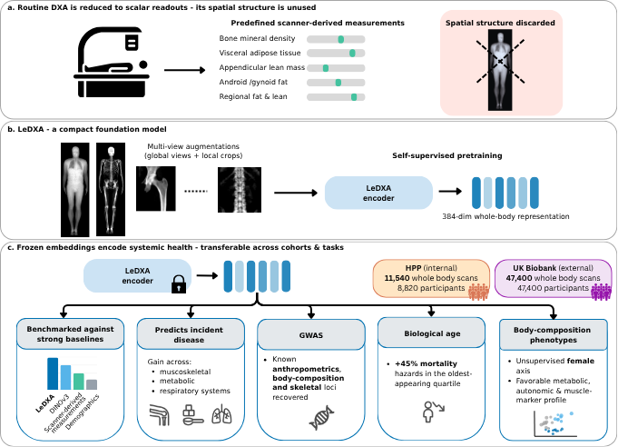
Figure 1 | LeDXA converts DXA scans into representations that encode systemic health. a, Routine DXA is reduced to a set of scalar readouts (bone mineral density, visceral adipose tissue, appendicular lean mass, android/gynoid fat, regional fat and lean), the spatial structure of the scan is left under-utilized. b, LeDXA is a compact self-supervised foundation model. Each whole-body scan is expanded into multi-view augmentations (2 global views and 8 local crops) and used to pretrain a ViT- Small/16 encoder, producing a 384-dimensional whole-body representation. c, The frozen embedding encodes systemic health and transfers across cohorts and tasks. Representations were learned on HPP (internal; 11,540 whole-body scans from 8,820 participants) and validated on UK Biobank (external; 47,400 whole-body scans from 47,400 participants). Across downstream tasks, LeDXA was benchmarked against strong baselines (DINOv3, scanner-derived measurements, and demographics), predicted incident musculoskeletal, metabolic, and respiratory disease, recovered known body-composition and bone loci from a genome-wide association study of its embeddings, stratified all-cause mortality (a 45% higher hazard in the oldest-appearing quartile), and recovered body-composition phenotypes including an unsupervised female axis linked to a favorable metabolic, autonomic, and muscle-marker profile.

Results

The results progress from recovering familiar scan measurements to disease prediction, genetics, an age-associated score and exploratory clustering. The following sections explain what each evaluation can establish.

Study populations and DXA imaging

Training uses 11,540 scans from 8,820 Human Phenotype Project participants. The frozen encoder is evaluated on a separate UK Biobank cohort with 47,400 scans. Repeated scans and participants are different counting units. Cohort filtering and missing outcomes make the actual sample smaller for individual analyses; the external cohort contributes no encoder-pretraining images.

LeDXA predicts multi-system disease and physiological markers

The learned vectors recover conventional composition measurements and support age, biomarker and disease predictors. AUROC measures how well a classifier ranks cases above non-cases; 0.5 is chance and 1 is perfect ranking. LeDXA significantly beats tabular measurements for 12 of 37 internal and 9 of 28 external disease endpoints, with ties or occasional losses elsewhere. All feature-based disease models also receive age, sex and body mass index. These are supervised downstream tests of an initially self-supervised encoder.
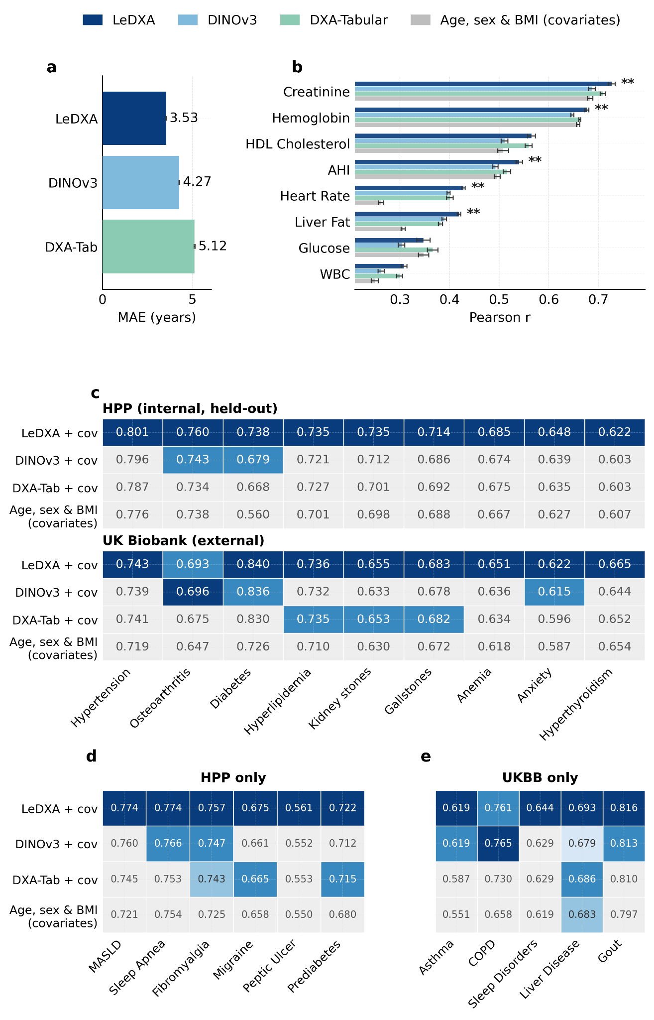
Figure 2 | LeDXA predicts prevalent disease and physiological traits. a, Chronological-age prediction in HPP. Models were fitted using ridge regression. Bars show mean absolute error (MAE, years) across 10 random held-out splits, and error bars denote standard error. b, Prediction of eight continuous physiological biomarkers in HPP. Models were fitted as in a. The covariate-only baseline used age, sex, and BMI alone. Bars show mean Pearson correlation across 10 splits. Asterisks indicate LeDXA significantly outperformed all competing models (two-sided Wilcoxon signed-rank test). c, Disease- classification area under the receiver operating characteristic curve (AUROC) for chronic conditions present in both the internal (HPP) and external (UKBB) cohorts, using the frozen HPP-trained encoder. All models were covariate-adjusted for age, sex, and BMI (Methods). Values show mean AUROC across 10 random splits. Within each endpoint, the winning model is shown in dark blue; models not significantly outperformed by the winner remain in lighter blues by rank, while significantly worse models are grayed out (two-sided Wilcoxon signed-rank test, FDR-adjusted P < 0.05) d, Disease-classification AUROC for HPP-specific conditions. e, Disease-classification AUROC for UKBB-specific conditions. In d and e, models, color scale, split structure, and significance criteria are as in c.

Longitudinal risk prediction of incident disease

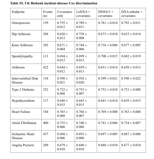
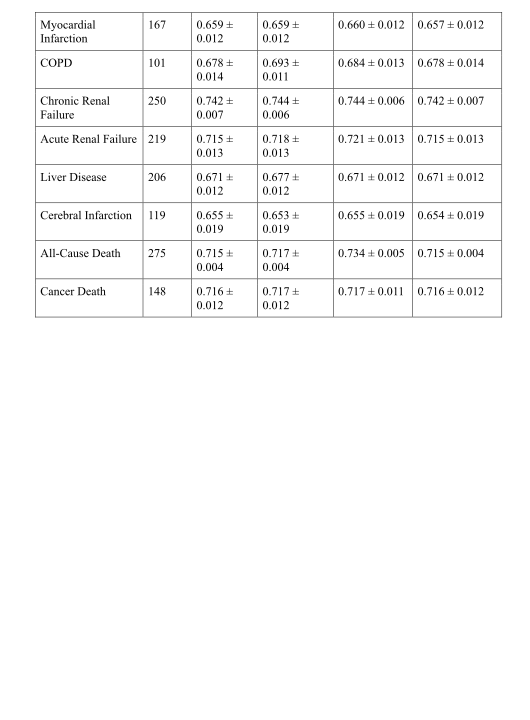
Here the scan precedes a recorded diagnosis. Cox models rank future event risk while accounting for different follow-up times. LeDXA improves over the tabular baseline on 9 of 20 tested endpoints; hip and knee arthrosis show the largest gains. Capturing 66% of hip cases in the highest-risk quarter describes case concentration, not 66% diagnostic accuracy or proof that screening improves outcomes. LeDXA and DINOv3 are similar on most incident endpoints.
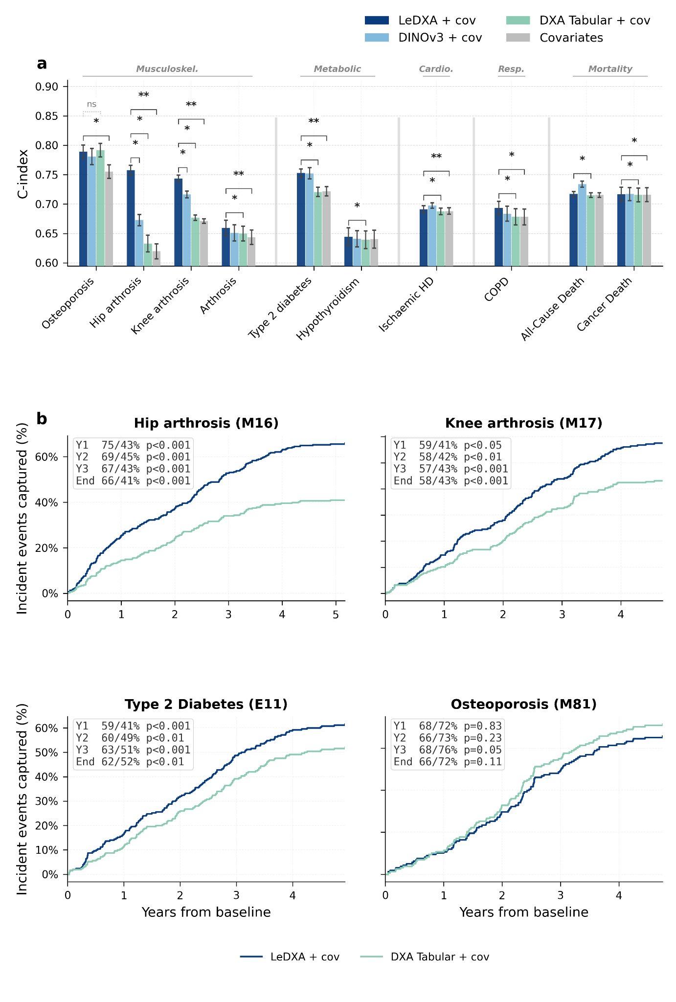
Figure 3 | LeDXA improves longitudinal prediction of incident disease in an external cohort. a, Discrimination of incident disease from baseline DXA scans. The plot displays 10 endpoints: the 9 conditions where LeDXA outperformed the DXA-tabular baseline (FDR-adjusted P < 0.05) out of 20 tested ICD-10 endpoints, alongside osteoporosis. Cox proportional-hazards models were trained using frozen LeDXA embeddings, DINOv3 embeddings, scanner-derived tabular DXA features, or covariates alone. All models (except the covariate-only baseline) included age, sex, and BMI as covariates. Participants with prevalent disease at baseline were excluded for each endpoint. Bars show the mean concordance index (C- index) across 10 random splits, and error bars denote standard error. Significance brackets indicate pairwise comparisons with LeDXA using two-sided Wilcoxon signed-rank tests with Benjamini–Hochberg FDR correction (*FDR-adjusted P < 0.05, **FDR-adjusted P < 0.01, ns = not significant). Endpoints are grouped by organ-system category. b, Cumulative case capture in the highest predicted-risk quartile (Q4), assigned at baseline, over follow-up, for four representative endpoints: hip arthrosis, knee arthrosis, type 2 diabetes, and osteoporosis. Lines show the cumulative fraction of incident events captured in Q4 for LeDXA (blue) and tabular DXA (green), both including covariates. Insets report the sensitivity of each model at years 1, 2, 3, and at the end of follow-up. p-values compare Q4 sensitivity between models using paired bootstrapping at each timepoint

LeDXA-derived representations match known genetic signals in an external cohort

A genome-wide association study asks whether common genetic variants correlate with components of the image vectors. Many matches overlap known body-composition and bone loci. LeDXA components show more estimated common-variant heritability than DINOv3 components. This supports biological alignment of some variation, while neither a statistical association nor mapping a variant to a nearby gene establishes a causal biological mechanism.
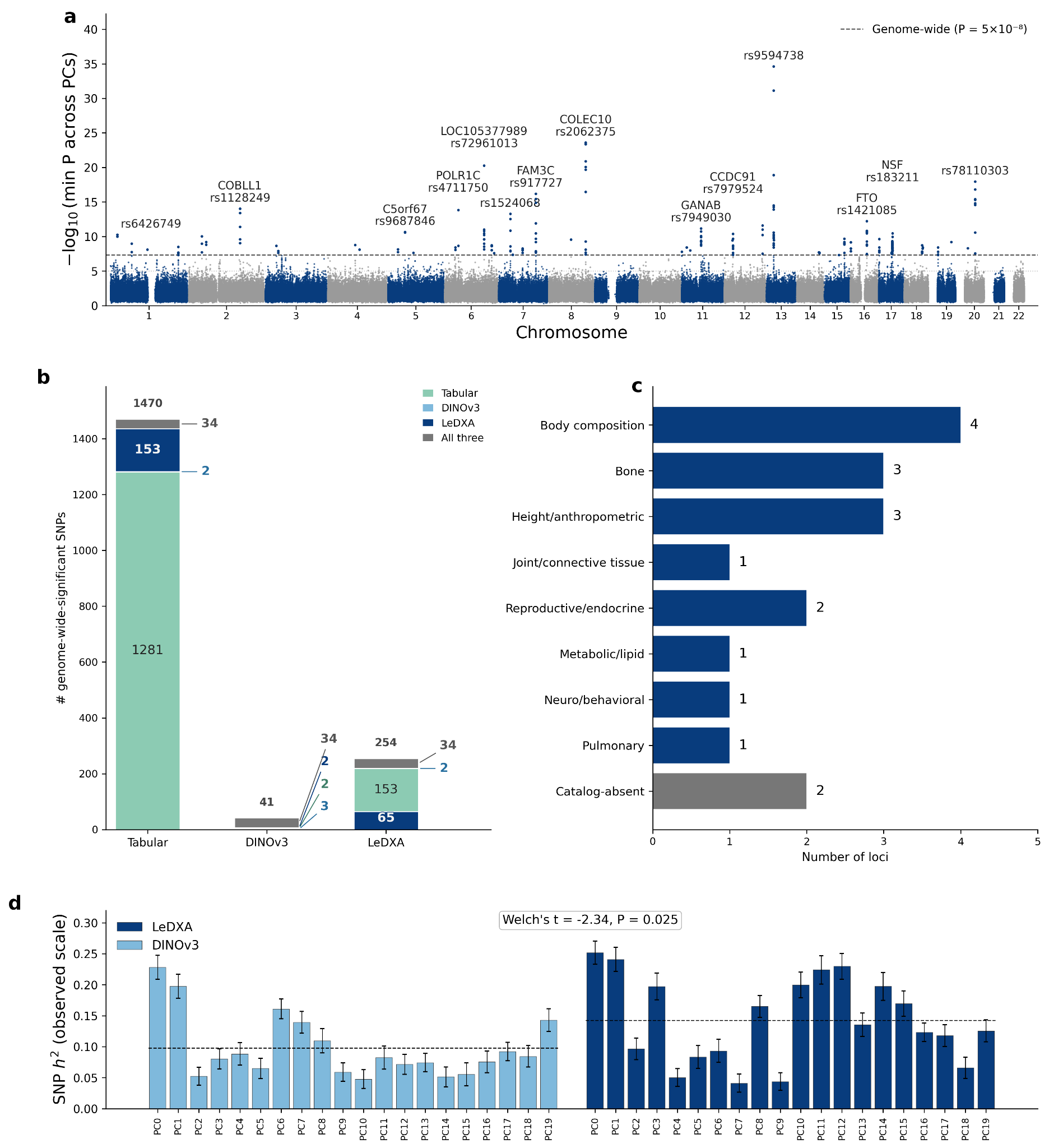
Figure 4 | LeDXA embeddings capture heritable common-variant architecture and recover established body-composition and skeletal loci. Genome-wide association studies (GWAS) were conducted in the UK Biobank on the leading 20 principal components (PCs) of the frozen image embeddings (LeDXA and DINOv3) and on scanner-derived tabular DXA traits. a, Manhattan plot for the LeDXA embedding GWAS, showing the minimum association P-value per genetic variant across the 20 PCs. Dashed line denotes genome-wide (P = 5 × 10⁻⁸) significance threshold. b, Number of genome-wide- significant single-nucleotide polymorphisms (SNPs; P < 5 × 10⁻⁸) by tabular traits, DINOv3, and LeDXA. Stacked segments partition the identified SNPs into method-specific and shared sets. c, Primary GWAS- Catalog trait domain for each of the 18 LeDXA-specific loci (500-kb LD clumping of the 65 LeDXA- specific genome-wide-significant SNPs). Each locus was assigned a single organ-system domain from the catalogued associations of its lead SNP — with 1000 Genomes European LD proxies (r² ≥ 0.8) used only where the lead SNP was itself uncatalogued — preferring its strongest association; the two loci with no catalogued association in any domain are shown separately as "Catalog-absent." d, SNP heritability (LD- score regression, observed scale; h²) for the 20 PCs from LeDXA and DINOv3. Error bars indicate LD- score-regression standard error, and dashed lines represent the mean per method (Welch’s two-sided t-test).

LeDXA-derived biological age predicts clinical outcomes and tracks pharmacological responses

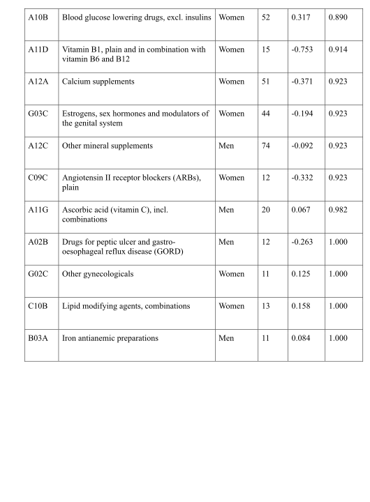
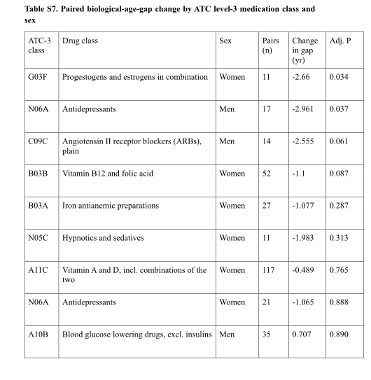
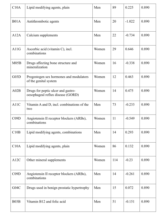
A supervised age predictor is corrected for its systematic relationship with chronological age; its residual becomes the age gap. An older-looking scan is associated with greater disease burden and higher mortality hazard after the stated adjustments. The gap is a constructed score rather than a direct measurement of a universal biological clock. Medication comparisons are small, uncontrolled before/after analyses: 11 women for hormone replacement and 17 men for antidepressants. They cannot show that either treatment reverses aging.
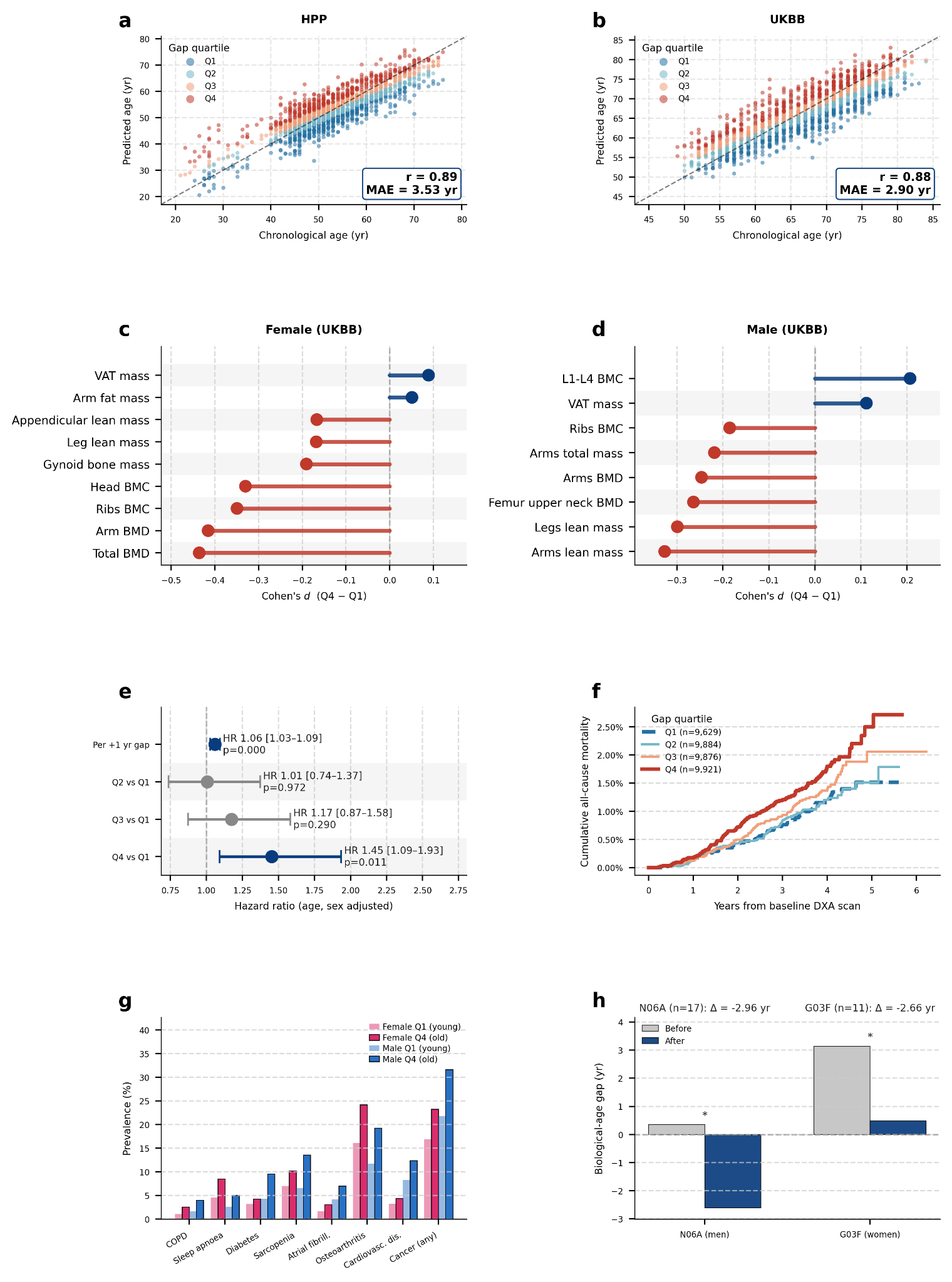
Figure 5 | LeDXA-derived biological-age gap captures sex-specific morphology, disease burden, mortality risk, and medication-associated change. a,b, Chronological-age prediction from LeDXA embeddings in the internal (HPP) and external (UKBB) cohorts. Predicted age was generated out-of-fold. The biological-age gap was defined as the residual after regressing predicted age on chronological age and chronological age squared. Points are colored by biological-age-gap quartile, with Q1 representing younger-appearing and Q4 representing older-appearing DXA morphology. Dashed lines indicate the identity line; boxed annotations report the Pearson correlation coefficient (r) and mean absolute error (MAE). c,d, Sex-stratified DXA phenotypes associated with biological-age-gap quartiles in UKBB. Lollipop plots show Cohen’s d comparing Q4 with Q1 (positive values indicate higher measurements in Q4). Displayed phenotypes represent the DXA-derived traits with the largest absolute effect sizes per sex (all displayed associations FDR-adjusted P < 0.05). e, Age- and sex-adjusted Cox proportional-hazards models for all-cause mortality in the UKBB mortality analytic cohort (n = 39,310; 377 deaths; median follow-up, 3.40 years). Points indicate hazard ratios (HRs) for each quartile relative to Q1, and horizontal lines indicate 95% confidence intervals (CIs). f, Cumulative all-cause mortality in the same UKBB cohort stratified by baseline biological-age-gap quartile. g, Prevalence of selected diseases in UKBB by sex and biological-age-gap quartile. Bars display the eight conditions with the largest mean prevalence ratio (PR) between Q4 and Q1 among the 17 evaluated conditions that reached significance (FDR-adjusted P < 0.05). h, Paired before/after analysis of biological-age-gap changes following the first reported initiation of significant Anatomical Therapeutic Chemical (ATC) level-3 medication classes in HPP participants with serial DXA scans.

Unsupervised LeDXA embeddings identify a lean- and high-bone-density female phenotype associated with favorable physiological profiles

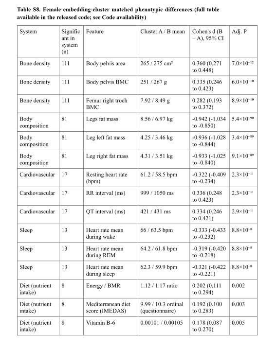
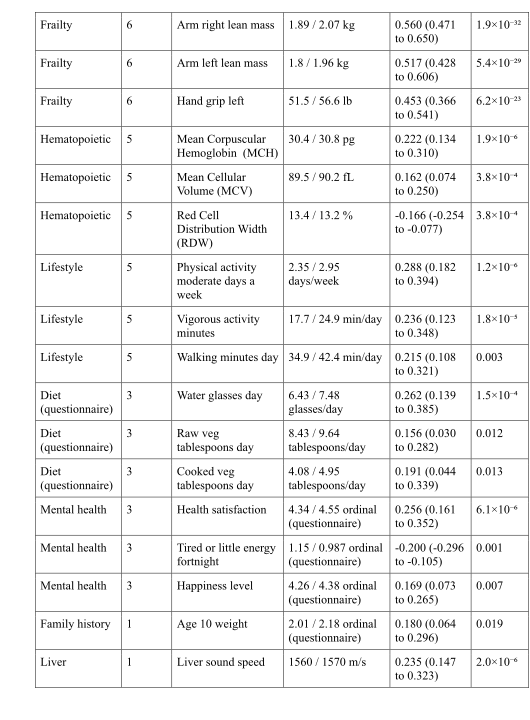
The authors project female scan vectors to two dimensions and cluster them, then match the groups on age and body mass index. One group has more lean tissue and higher bone density, alongside several favorable measured traits. Matching reduces two specific confounders, but does not randomize the groups. Because clustering happens after a nonlinear two-dimensional projection, the visible groups also depend on the analysis pipeline.
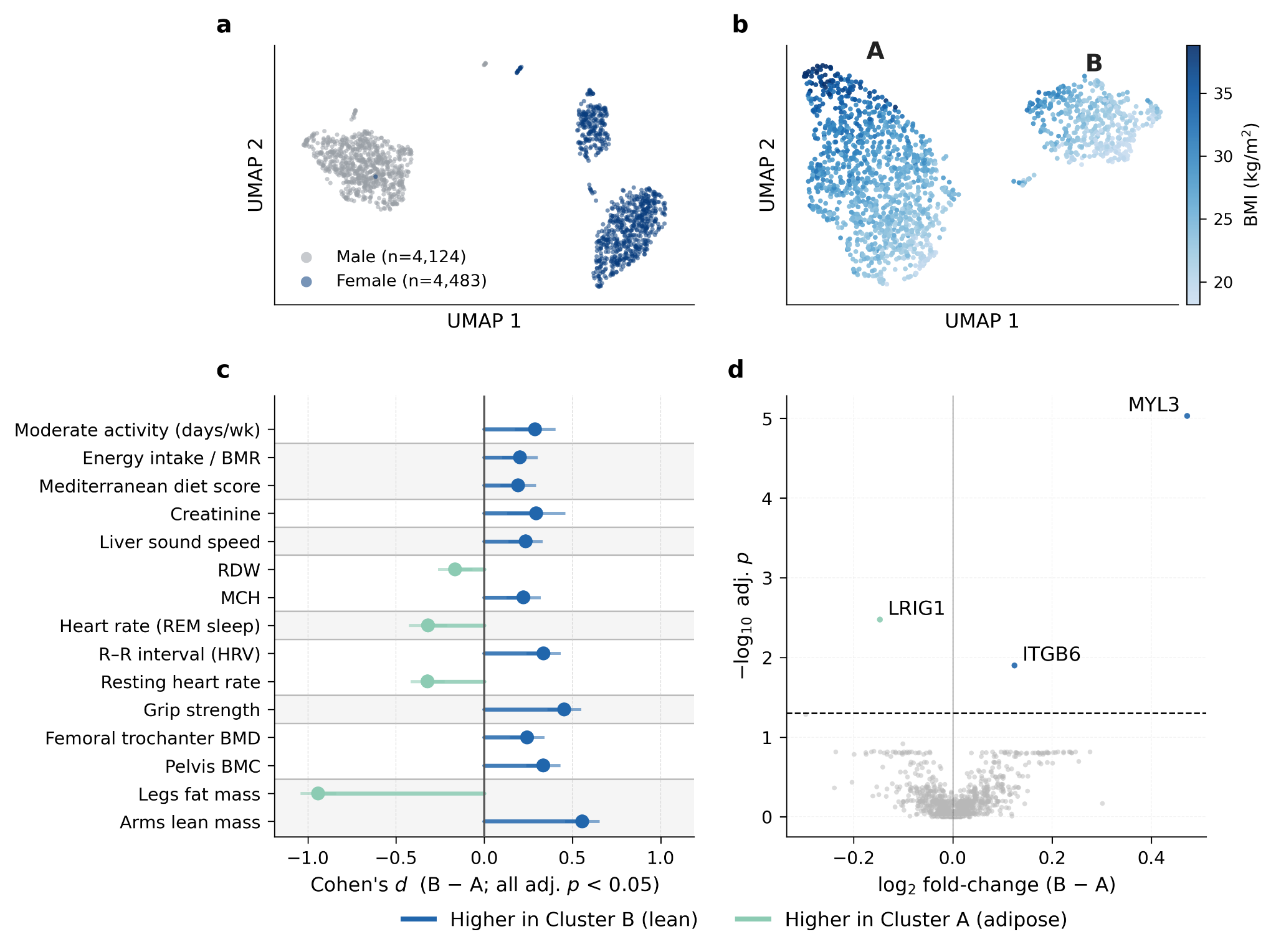
Figure 6 | Unsupervised clustering of LeDXA embeddings identifies a female body- composition axis. a, Uniform manifold approximation and projection (UMAP) of whole-body DXA embeddings from the Human Phenotype Project (HPP), colored by sex. b, UMAP of female HPP participants colored by body mass index (BMI). c, Phenotypic differences between Cluster B and Cluster A following 1:1 Mahalanobis-distance matching on age and BMI (yielding 1,035 matched pairs). Lollipop plots display Cohen’s d (Cluster B minus Cluster A), with positive values indicating higher measurements in Cluster B. Displayed associations are significant at FDR-adjusted P < 0.05. d, Plasma-proteomic differential-abundance analysis in the matched cohort utilizing the Olink platform. The x-axis represents the log₂ fold-change between clusters (Cluster B minus Cluster A), and the y-axis indicates the −log₁₀ (FDR- adjusted P-value).

Discussion

The engineering lesson is that a small model trained on the right imaging domain can preserve useful spatial information that scalar summaries lose. External-cohort evaluation is a strength. Important limits include selected volunteer cohorts, observational outcomes, self-reported diagnoses or medication histories, scanner differences and untested clinical utility. The embeddings are promising research features, with deployment and treatment decisions requiring additional evidence.

Methods

The methods distinguish encoder pretraining from supervised task fitting. Read this part to understand which labels, covariates, cohort filters and tuning choices enter each reported result.

Study populations

Internal participants come from an Israeli longitudinal cohort and external participants from UK Biobank. Eligibility, image completeness, covariates and outcome availability define each analysis set. Subject-level splits keep repeated scans from the same person out of both training and validation within a split; the findings still reflect the populations and scanners represented here.

Data acquisition and preprocessing

Bone and soft-tissue images are resized and replicated into three channels. Regional femur and lumbar scans supplement the full-body inputs for relevant tasks. This standardizes the input tensor while preserving the distinction between full-body and clinically targeted views.

Self-supervised pretraining with LeJEPA

A small vision transformer turns each crop into features, and a projection network supplies the training coordinates. Two global views and eight local crops of a scan are encouraged to agree. SIGReg pushes projected coordinates toward a standard Gaussian distribution so different examples cannot all collapse to the same point. This is crop-based representation learning, without future-state prediction or diagnosis labels in pretraining. The exact source equations remain below.

Equations

Original LeJEPA formula 1 from page 23
Original LeJEPA formula 2 from page 23
Original LeJEPA formula 3 from page 23

Training configuration

Training uses AdamW, 400 epochs, mixed precision and a single NVIDIA L40S graphics processor, taking approximately 10 hours under the stated setup. Once trained, the encoder is frozen and bone/soft-tissue vectors are extracted deterministically. Downstream models operate on these features rather than updating the encoder unless a separate fine-tuning experiment explicitly does so.

Baseline models

The general-image comparison is frozen DINOv3; the tabular comparison uses scanner-derived measurements. Age, sex and body mass index are included consistently in the relevant feature-based tasks. Numerical preprocessing and model selection are fitted within the specified splits. These are comparisons of complete feature-and-readout pipelines, not encoder architecture alone.

Downstream evaluation in HPP

Linear or regularized readouts predict continuous traits and binary diagnoses. Hyperparameters are selected within subject-disjoint training folds, and performance is repeated across ten random splits. A separate end-to-end fine-tuning sensitivity study updates both image models under a shared protocol. Organ-system labels aggregate diagnoses using the supplementary mapping, which differs from testing each individual disease.

UKBB cross-sectional disease classification

The external encoder remains frozen, but the external cohort supplies labels for fitting and validating a new logistic-regression readout. External transfer of an encoder therefore does not mean a complete classifier trained only in the original cohort. The four comparison arms use the same subject split and applicable covariates.

Longitudinal incident-disease risk

Participants with the endpoint already recorded at baseline are excluded. Penalized Cox models use scan features and covariates, with tuning and repeated holdout evaluation. A concordance index measures ordering of event risk; censoring handles follow-up that ends before an event is observed. Top-quartile case capture provides another view of ranking, without establishing a treatment threshold or net clinical benefit.

Biological age

Out-of-fold age predictions avoid predicting a person using a regressor fitted on that person. Removing linear and quadratic dependence on chronological age constructs the gap; near-zero age correlation is consequently partly by design. Subsequent analyses compare phenotypes, disease prevalence, mortality and medication-associated change, with their own models and adjustments. Residual confounding and small medication groups remain relevant.

Statistical analysis

Regression uses correlation and classification uses AUROC. Multiple-testing correction limits the expected fraction of false discoveries among declared discoveries under its assumptions; an adjusted significance threshold does not measure effect size or practical importance. Repeated splits reuse many participants, so the reported variation across splits is different from collecting ten independent cohorts.

Equation

Original false-discovery-rate expression, part 1Original false-discovery-rate expression, part 2

Clustering

The pipeline standardizes features, reduces them with principal components, creates a two-dimensional UMAP map and fits two clusters there. Outlier filtering precedes one-to-one matching on age and body mass index. Molecular comparisons use platform-specific subsets with different sample sizes. These choices make the cluster analysis exploratory and dependent on the representation, projection and matching procedure.

Genome-wide association of embedding space

The study tests the leading 20 image-vector components against genetic variants after quality control and adjustment for demographic and genetic ancestry components. Nearby correlated variants are grouped into loci. Heritability estimates concern variance explained by measured common variants under the analysis model. Comparing principal components of image features with individual tabular traits is informative, but those are different phenotype constructions.

Data availability

Research access to the Human Phenotype Project data requires its stated institutional application process. The paper does not make individual medical scans freely downloadable.

Code availability

The authors link their implementation and released result tables. The exact pinned manuscript, rather than a changing repository, is the authority for this edition’s reported protocol.

Acknowledgments

Funding and acknowledgments are retained in the source text. They do not form part of the method or evaluation evidence.

Additional information

The original manuscript identifies the corresponding author. The reading edition preserves the paper’s provenance and complete bibliography.

Figure S1 — Architecture and evaluation setup

The diagram separates crop-based, label-free pretraining from supervised downstream readouts. SIGReg regularizes projected training coordinates; the final frozen encoder supplies the scan features.
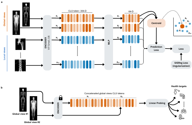
Figure S1 | LeDXA architecture and evaluation setup. a, Self-supervised pretraining with LeJEPA objective. Every DXA scan has two images: a bone image and a soft-tissue image, which are handled the same way. Each image is turned into 10 augmented views — 2 whole- body (global) views and 8 close-up (local) views (the femur/spine regional scans plus small random crops drawn from the whole body scan crops). A ViT-Small/16 shared encoder turns each view into a 384-dimensional representation (x1–x10), and a small 3-layer network compresses these to 64 dimensions (z1–z10). Training pushes every view's representation toward the average of the two global views, while a sketched isotropic gaussian regularization (SIGReg) term keeps the overall spread of representations close to a standard Gaussian distribution. b, The trained encoder is then frozen (its weights are not changed). For each scan, the bone and tissue representations are concatenated together and fed to a simple linear model that is trained to predict health outcomes.

Figure S2 — Cohort selection

Follow the participant counts through image availability and completeness filters. The external pretraining exclusion and task-specific analytic sample sizes answer different questions.
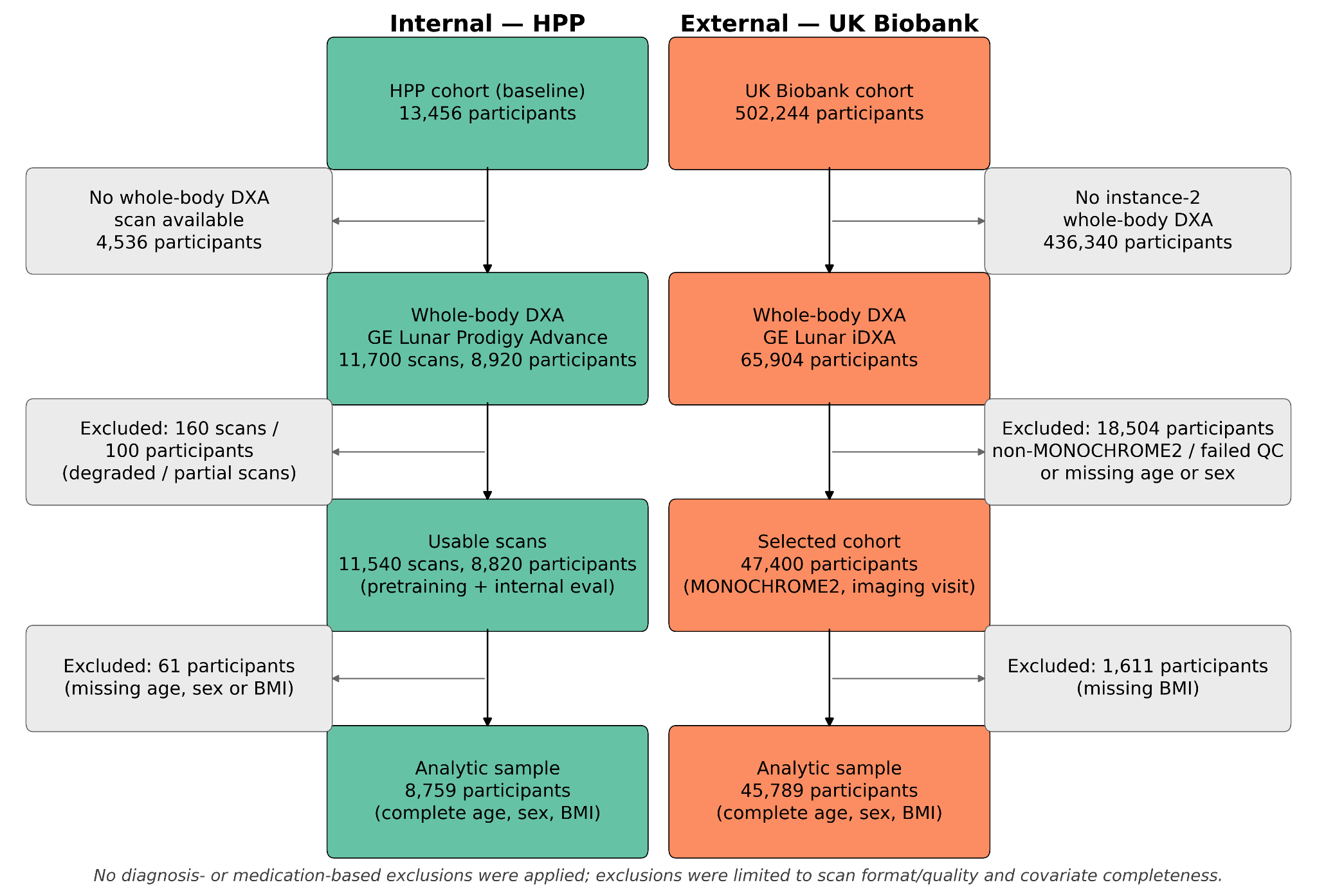
Figure S2 | Study flow and cohort selection. Participant flow for the internal Human Phenotype Project (HPP; green, left) and external UK Biobank (UKBB; orange, right) cohorts, detailing the progression from baseline enrollment to the final covariate-complete analytic samples. Colored boxes represent the cohorts retained at each step, while grey boxes indicate the number of excluded scans or participants alongside the reason for exclusion. For the HPP cohort, counts are provided for both dual-energy X-ray absorptiometry (DXA) scans and unique participants, as self-supervised pretraining utilized all available longitudinal scans, whereas the downstream analytic sample is defined at the participant level. UKBB counts are provided strictly per participant. Exclusions for both cohorts were limited to the availability of a usable whole-body DXA scan (format and image quality) and the completeness of baseline covariates (age, sex, and body mass index); no additional diagnosis- or medication-based exclusions were applied. QC, quality control.

Figure S3 — Recovering conventional scan measurements

Reconstructing familiar scanner readouts checks whether the features retain known information. Bone-density classification also uses regional scans; it is not the same input protocol as every full-body task.
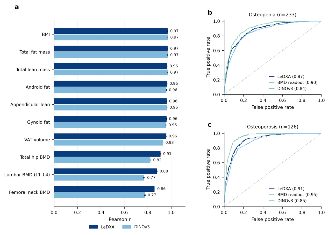
Figure S3 | LeDXA recovers DXA-derived phenotypes from raw images (HPP). a, Recovery of ten scanner-measured anthropometric and DXA quantities (body-mass-index, total fat mass, total and appendicular lean mass, android and gynoid fat, visceral adipose tissue (VAT) volume, and femoral-neck, total-hip and lumbar (L1–L4) bone-mineral density (BMD)) by the LeDXA and DINOv3 imaging embeddings (Pearson r between predicted and measured values; bars, mean over 10 random 80/20 subject-level splits; error bars, standard error of the mean). b, c, Receiver-operating-characteristic (ROC) curves for recovering self-reported osteopenia (b, n = 233) and osteoporosis (c, n = 126) from the LeDXA and DINOv3 embeddings, compared with a model trained on the scanner-derived BMD measurements. Legend values are the mean area under the ROC curve (AUROC); n, number of positive cases. Across the seven non-bone measures, both embeddings performed comparably (mean ± SD Pearson r: LeDXA 0.964 ± 0.005, DINOv3 0.957 ± 0.016), with LeDXA modestly ahead on VAT volume (0.96 vs. 0.93). On the three diagnosis-defining BMD sites, LeDXA scored higher than DINOv3 (0.882 ± 0.026 vs. 0.789 ± 0.029), mirroring its advantage over DINOv3 on the bone diagnoses in b, c.

Figure S4 — Organ-system disease prediction

Grouping diagnoses tests broader outcome categories. Categories contain different numbers and mixtures of diseases, so their scores cannot be interpreted as equally difficult tasks.
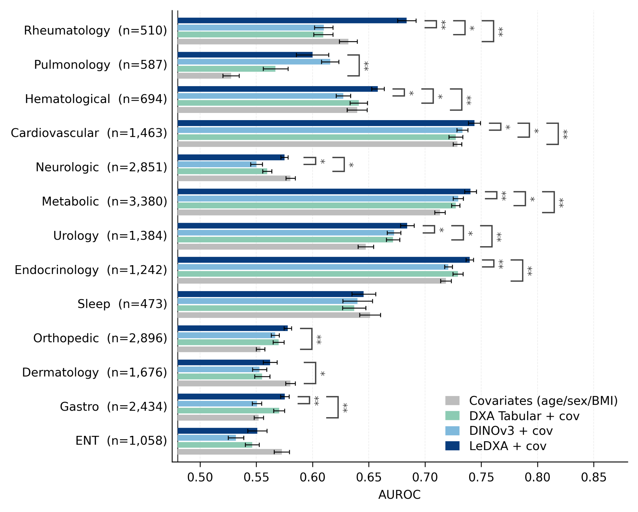
Figure S4 | LeDXA’s disease-predictive advantage across organ systems (HPP). Mean AUROC for classifying organ-system-level disease endpoints in the HPP cohort. The performance of four models is compared: the LeDXA embedding, the general-purpose DINOv3 embedding, scanner-derived DXA-tabular features, and a covariate-only baseline (age, sex, and BMI). For the three main models, age, sex, and BMI were concatenated alongside the primary features (Methods). Individual diagnoses were grouped into 13 chronic organ-system categories (Methods; Table S4); a subject was labeled positive for a group if affected by any constituent diagnosis. Bars show the mean AUROC across 10 random 80/20 subject-level train/test splits, and error bars represent the standard error of the mean. The number of positive cases per group is indicated by n. Brackets denote two-sided Wilcoxon signed-rank tests across seeds, adjusted via the Benjamini–Hochberg FDR procedure across groups, comparing LeDXA with each of the other three arms (*adjusted P < 0.05, **adjusted P < 0.01). LeDXA significantly exceeds the DXA-tabular baseline in 6 of 13 groups, led by cardiovascular, hematological, metabolic, neurologic, rheumatological, and urological systems, indicating that the raw imaging representation carries systemic disease-predictive information not fully captured by predefined scalar DXA measurements.

Figure S5 — Fine-tuning sensitivity

Updating the encoders under a shared supervised protocol broadly preserves the comparison on eight selected targets. This sensitivity experiment is distinct from the main frozen-feature results.
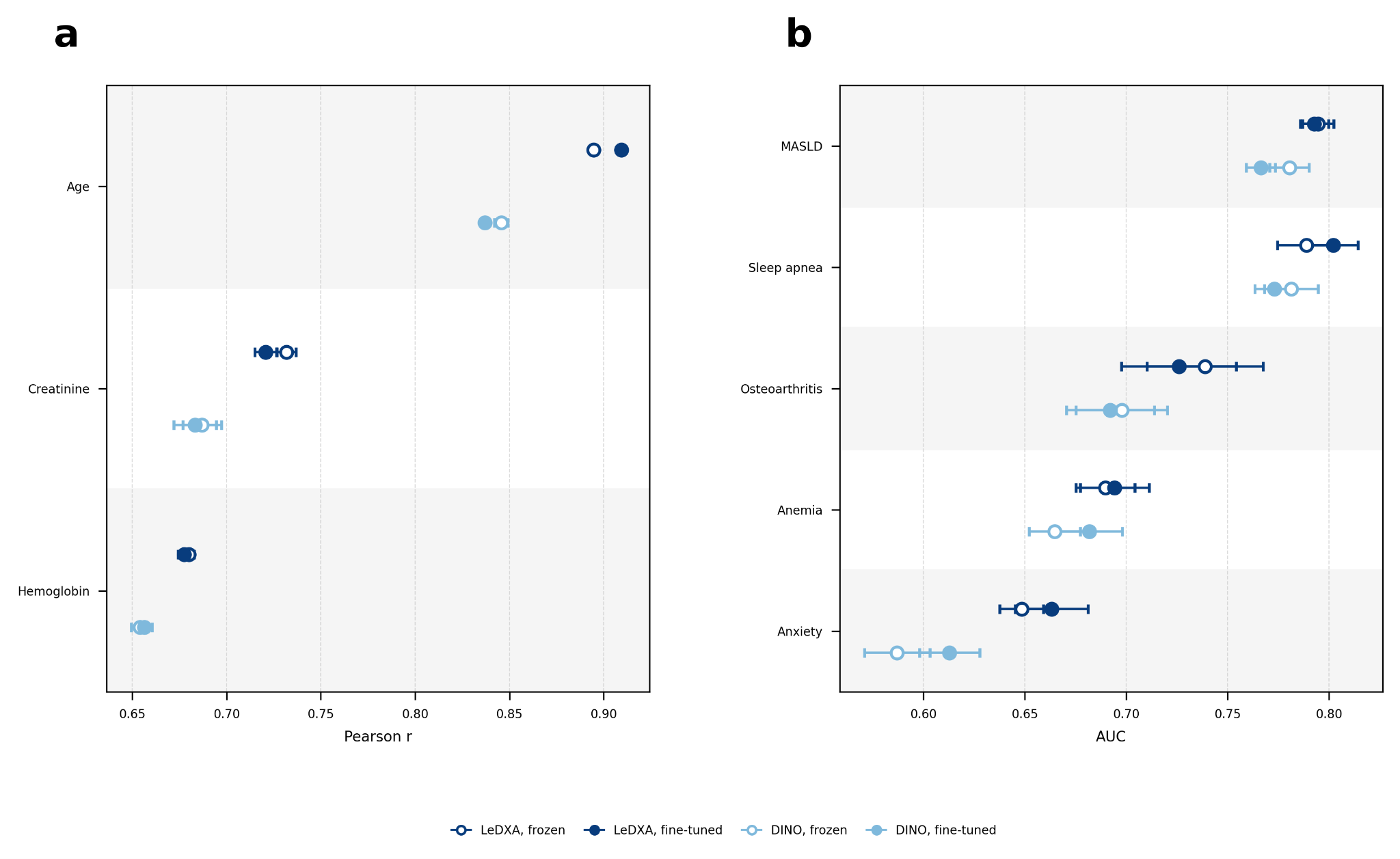
Figure S5 | Supervised fine-tuning does not change model performance rankings. Frozen linear probing (open markers) versus full end-to-end supervised fine-tuning (filled markers) for LeDXA and DINOv3, using embeddings alone (no age/sex/BMI covariates). Data represent mean ± standard error of the mean (s.e.m.) across 5 random seeds. a, Prediction of three continuous physiological biomarkers (chronological age, creatinine, and hemoglobin), evaluated by Pearson correlation (r). b, Classification performance (area under the receiver operating characteristic curve [AUROC]) for five prevalent conditions in the Human Phenotype Project (HPP) cohort: metabolic dysfunction-associated steatotic liver disease (MASLD), sleep apnea, osteoarthritis, anemia, and anxiety. Across all eight evaluated targets, supervised fine- tuning did not reverse the performance ranking of LeDXA relative to DINOv3 established under frozen probing.

Figure S6 — Age-gap detrending

The residual has little remaining correlation with chronological age after detrending. This is an intended property of the score construction, rather than independent proof that it measures aging correctly.
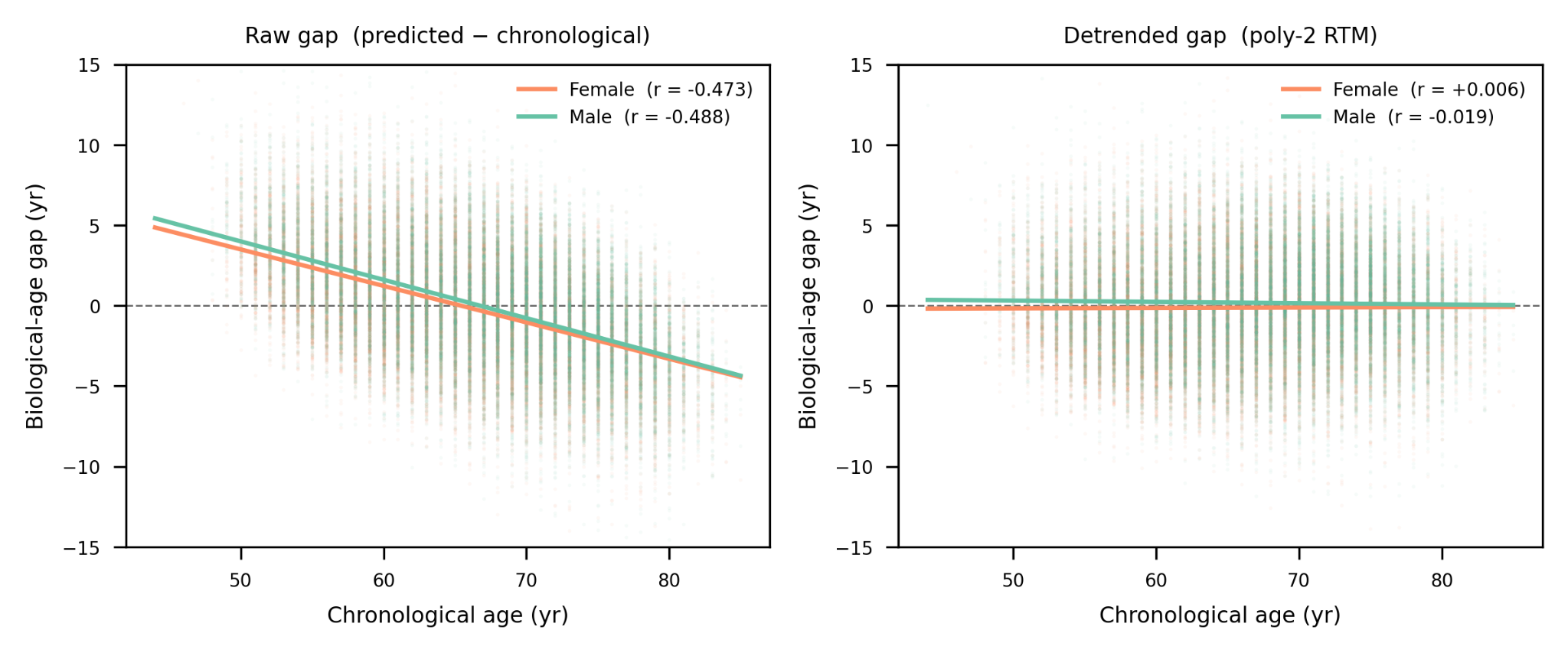
Figure S6 | Biological-age gap versus chronological age, by sex. Scatter of the detrended biological-age gap against chronological age in UK Biobank, showing negligible residual correlation within each sex.

Figure S7 — Internal replication of age-gap patterns

The internal cohort broadly reproduces selected directions of age-gap associations. This supports consistency of those associations, without converting them into causal effects.
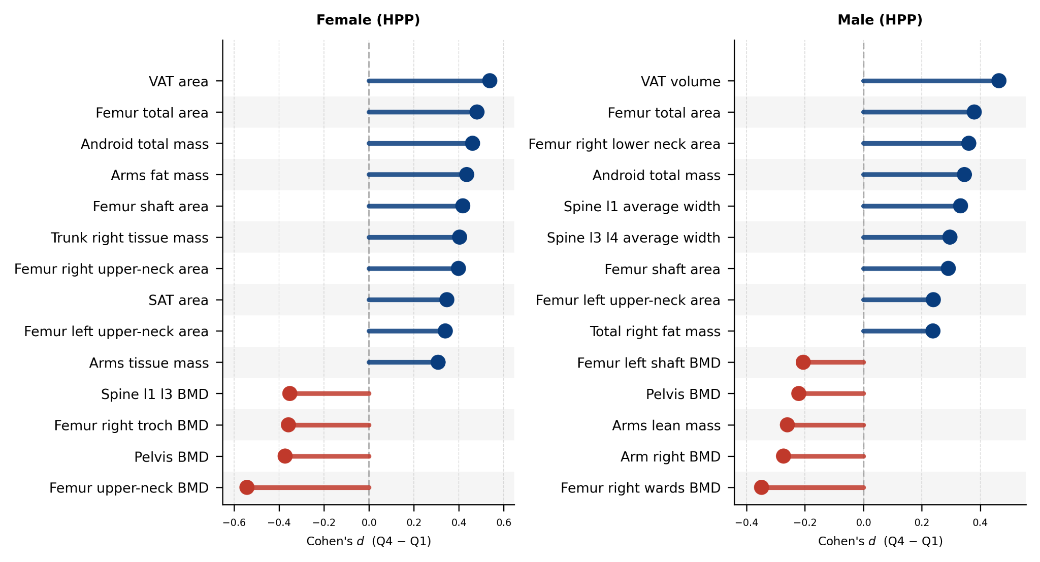
Figure S7 | HPP replication of the biological-age-gap Q4-vs-Q1 DXA body- composition associations. Cohen's d (Q4 − Q1) for the top false-discovery-rate-significant DXA body-composition and bone phenotypes in the HPP cohort, by sex, mirroring the UK Biobank analysis in Fig. 5c, d. Positive values indicate higher levels in the oldest-appearing (Q4) biological-age-gap quartile. Female n = 1,517 (Q1/Q4 = 380/380); male n = 1,221 (306/306). Higher visceral adipose tissue and lower femoral bone-mineral density in Q4 recapitulate the UK Biobank pattern.

Figure S8 — Disease prevalence across age-gap quartiles

The bars compare disease prevalence among people with younger- and older-looking scans. These are cross-sectional associations and differ from predicting newly occurring disease during follow-up.
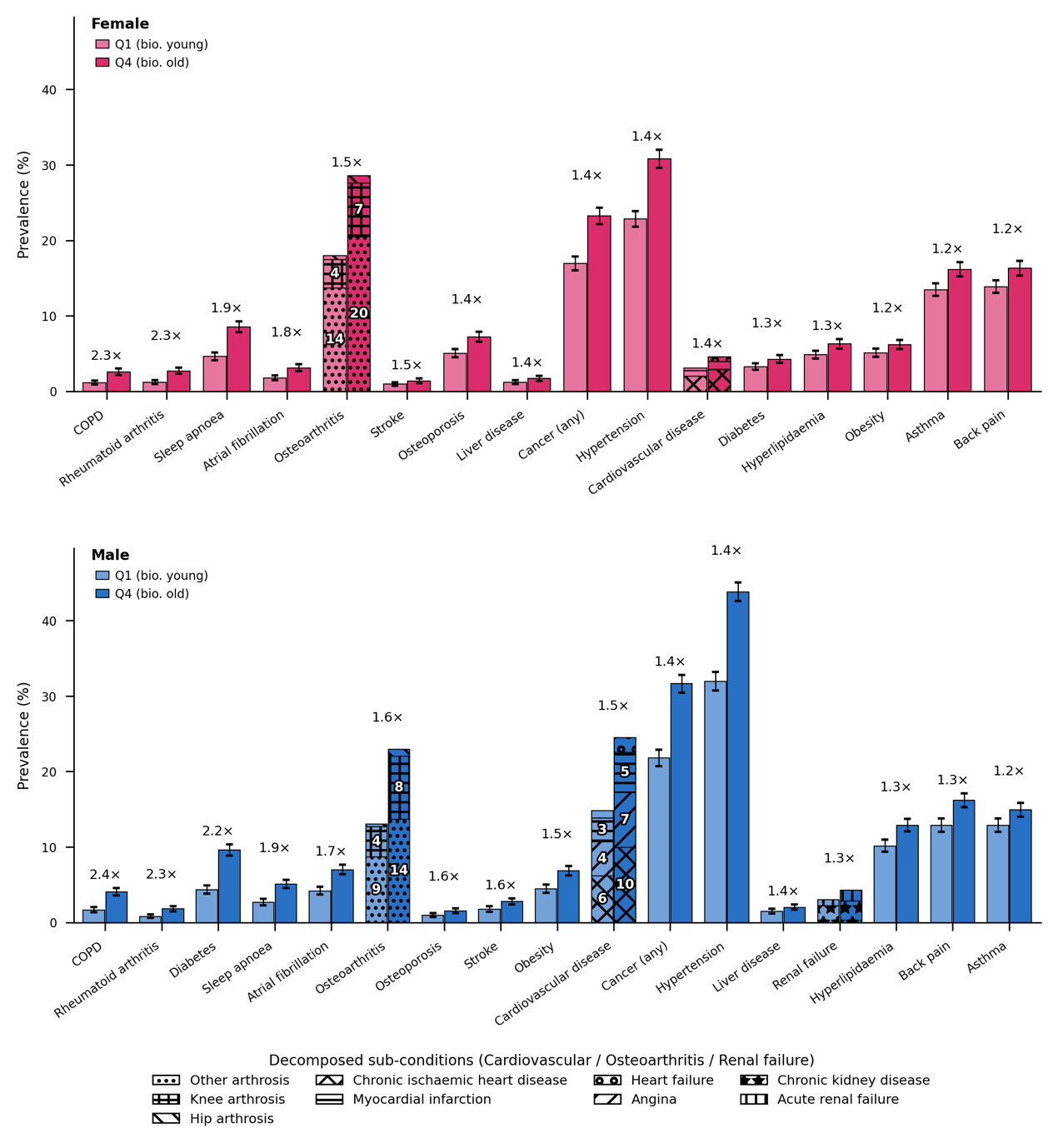
Figure S8 | Cross-sectional disease prevalence by LeDXA biological-age-gap quartile in UK Biobank. Prevalence of conditions present at the first imaging visit for participants in the lowest (Q1, biologically younger) versus highest (Q4, biologically older) quartile of the LeDXA biological-age gap, stratified by sex. The biological-age gap represents the residual of LeDXA-predicted age regressed on chronological age. A condition was considered prevalent if its earliest ICD-10/self-reported diagnosis preceded the imaging visit. Bars display percentage prevalence with 95% Wilson confidence intervals (error bars); values above each pair denote the Q4:Q1 prevalence ratio. Only conditions reaching significance (Benjamini–Hochberg false discovery rate (FDR) < 0.05, χ² test) are shown; groups with fewer than 20 assessable participants were omitted.Three composite categories—cardiovascular disease, osteoarthritis, and renal failure—are represented as stacked bars decomposed into their constituent sub-conditions. Bar fill indicates quartile (light = Q1, dark = Q4), while hatch patterns denote specific sub-conditions. In-bar numbers report the sub-condition's prevalence (%). Because sub-conditions are not mutually exclusive (e.g., a participant may have both angina and myocardial infarction), the summed height of a decomposed bar can modestly exceed the true prevalence of its composite category.

Table S1 — Cohort characteristics

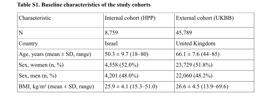
The cohorts differ in age, country, sex distribution and body composition. Reported sample sizes depend on the completeness filter used for this table; they need not equal all available scans.
Original Table S1, part 1 of 1, PDF page 44
Table S1. Cohort characteristics. Complete original table, including continuation pages.

Table S2 — Internal disease classification

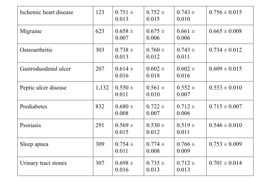
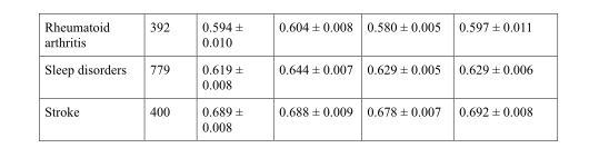
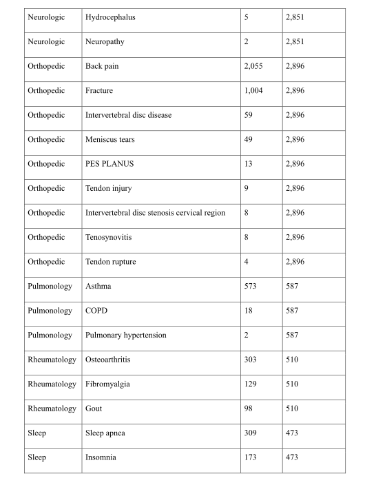
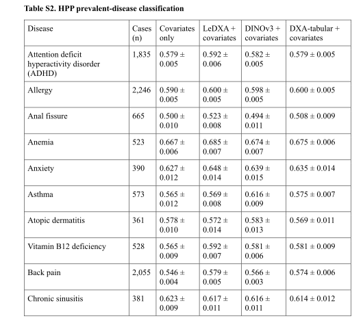
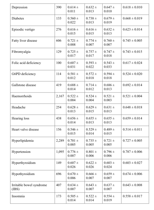
The full table includes wins, ties and losses across diseases. Read each AUROC alongside its case count, variation and covariate-adjusted baseline, rather than using selected examples alone.
Original Table S2, part 1 of 3, PDF page 44Original Table S2, part 2 of 3, PDF page 45Original Table S2, part 3 of 3, PDF page 46
Table S2. Internal disease classification. Complete original table, including continuation pages.

Table S3 — External disease classification

These results fit task readouts in UK Biobank using the frozen encoder. External feature transfer and external validation of a fully fixed diagnostic system are different evaluation designs.
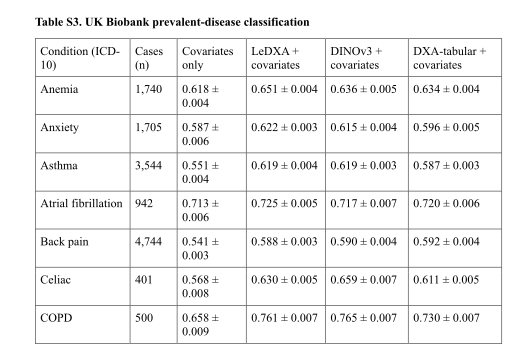
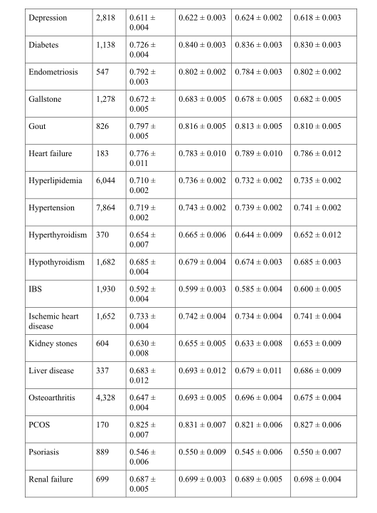
Original Table S3, part 1 of 3, PDF page 46Original Table S3, part 2 of 3, PDF page 47Original Table S3, part 3 of 3, PDF page 48
Table S3. External disease classification. Complete original table, including continuation pages.

Table S4 — Organ-system grouping

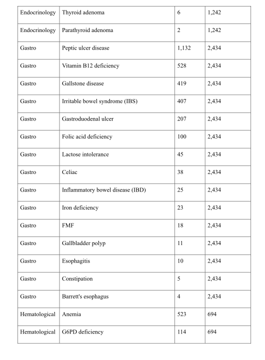
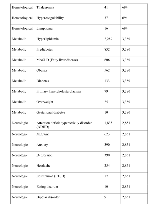
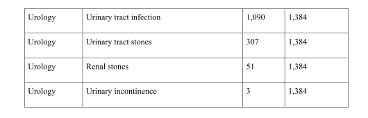
This mapping defines the aggregated labels used in the system-level analysis. A participant is positive when at least one included diagnosis is present.
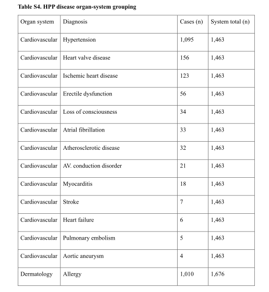
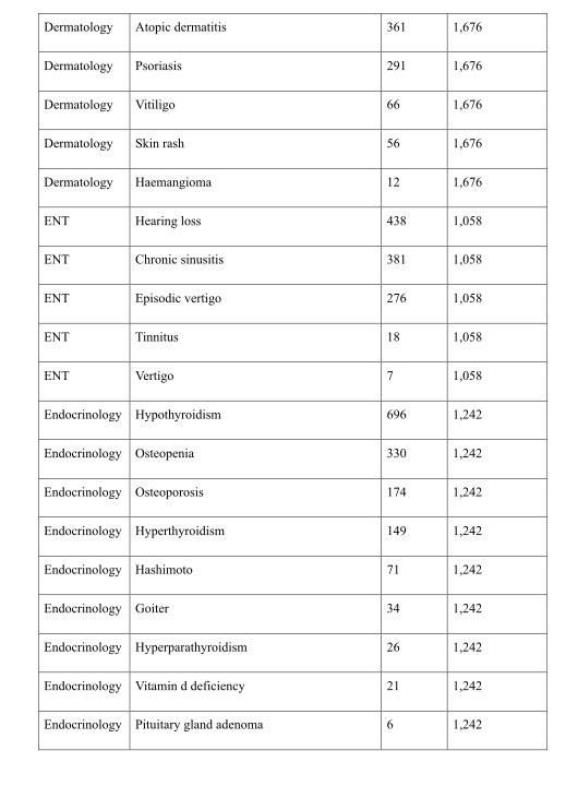
Original Table S4, part 1 of 6, PDF page 48Original Table S4, part 2 of 6, PDF page 49Original Table S4, part 3 of 6, PDF page 50Original Table S4, part 4 of 6, PDF page 51Original Table S4, part 5 of 6, PDF page 52Original Table S4, part 6 of 6, PDF page 53
Table S4. Organ-system grouping. Complete original table, including continuation pages.

Table S5 — Incident-disease risk

The complete concordance-index table shows the endpoint-specific picture, including outcomes without a LeDXA advantage. More accurate ranking does not by itself establish clinical utility.
Original Table S5, part 1 of 2, PDF page 53Original Table S5, part 2 of 2, PDF page 54
Table S5. Incident-disease risk. Complete original table, including continuation pages.

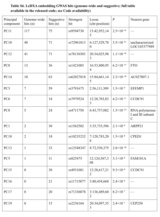
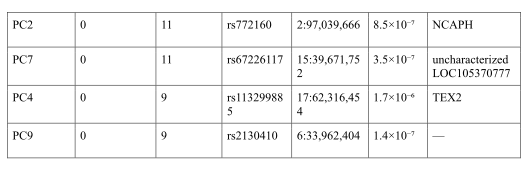
Table S6 — Genetic association hits

Variants and nearest-gene annotations help inspect known and representation-specific signals. Nearby-gene assignment and statistical association do not identify a proven causal gene.
Original Table S6, part 1 of 2, PDF page 55Original Table S6, part 2 of 2, PDF page 56
Table S6. Genetic association hits. Complete original table, including continuation pages.

Table S7 — Medication-associated age-gap change

The table retains all tested medication groups, including nonsignificant results and small paired samples. Before/after changes are observational and can reflect changes beyond the medication itself.
Original Table S7, part 1 of 3, PDF page 56Original Table S7, part 2 of 3, PDF page 57Original Table S7, part 3 of 3, PDF page 58
Table S7. Medication-associated age-gap change. Complete original table, including continuation pages.

Table S8 — Matched cluster phenotypes

These feature comparisons describe the two female clusters after matching on age and body mass index. Other differences can remain; matching is not random assignment.
Original Table S8, part 1 of 3, PDF page 59Original Table S8, part 2 of 3, PDF page 60Original Table S8, part 3 of 3, PDF page 61
Table S8. Matched cluster phenotypes. Complete original table, including continuation pages.

Table S9 — Cluster molecular measurements

Different molecular platforms cover different subsets. The table includes significant and suggestive comparisons, so the adjusted significance values matter when distinguishing supported findings.
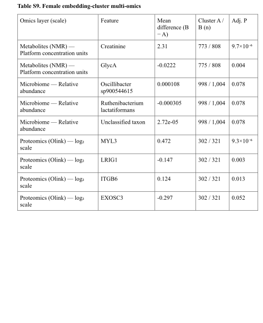
Original Table S9, part 1 of 1, PDF page 61
Table S9. Cluster molecular measurements. Complete original table, including continuation pages.

Table S10 — Scanner feature dictionary

The baseline combines body composition, bone density, geometry and related scanner quantities. The dictionary makes clear that this is a substantial measured-feature baseline, rather than only one bone-density number.
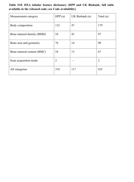
Original Table S10, part 1 of 1, PDF page 62
Table S10. Scanner feature dictionary. Complete original table, including continuation pages.
Concept demonstration

Open image ↗