HP-JEPA represents each graph at several partition resolutions and performs latent prediction independently within each resolution. Frozen resolution-specific graph features are then concatenated or combined with task-specific weights. The tested model improves over fixed-resolution Graph-JEPA on six of eight tasks. Its hierarchy is a bank of coarse-to-fine granularities, not an explicitly nested parent–child graph or a cross-resolution prediction loss.
1. Introduction
A single patch scale can hide small motifs in a large graph or fragment an already small graph too aggressively. The paper therefore retains several resolutions. The key questions are how to define valid tokens for different graph sizes, what latent quantity is predicted, and how downstream tasks combine the resulting representations.
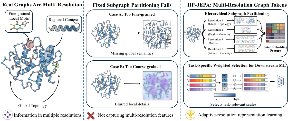
Figure 1. Motivation and overview of HP-JEPA.
Real-world graphs contain complementary structural information at
multiple resolutions, including fine-resolution local motifs,
intermediate-resolution regional context, and coarse-resolution
global topology.
A single fixed resolution can be overly fine, fragmenting global
context, or overly coarse, obscuring local structure.
HP-JEPA constructs graph-region tokens at multiple resolutions and
integrates their resolution-specific representations.
Task-specific resolution weighting allows downstream models to
emphasize the most informative resolutions.
2. Related Work
Related work separates graph contrastive learning, reconstruction and latent prediction. The comparison table summarizes mechanisms, but architectural categories do not substitute for matched benchmark evaluation. HP-JEPA’s direct baseline is a fixed-resolution graph JEPA.
Table 1. Design-level comparison of graph representation learning methods. The check marks (✓) and cross marks (✗) indicate that the property is explicitly satisfied/unsatisfied by design, and a triangle () indicates a partial match.
Notes.
(1) “No Neg.” means the objective does not require explicit negative pairs.
(2) “No Raw Recon.” means the method does not reconstruct raw node attributes, edges, or graph structure.
(3) “Latent Pred.” means the target is a representation-space target.
(4) “Region Tokens” means graph regions, subgraphs, or patches are explicit learning units.
(5) “Multi-Resolution Tokens” means that graph-region tokens are explicitly constructed at multiple partition resolutions.
(6) For F-GIN, check marks under “No Neg.” and “No Raw Recon.” only indicate that these mechanisms are absent; F-GIN is still supervised.
AD-GCL-FIX and AD-GCL-OPT are merged because they share the same method design.
3. Preliminaries
The preliminaries define graph-level representation learning and the context–target prediction problem. The distinction between pretraining without task labels and supervised downstream readout remains important.
3.1. Graph Representation Learning
A graph encoder maps node attributes and connectivity into a fixed-length representation. Downstream classification or regression trains a readout on those features. Multi-resolution tokenization changes what structural information reaches that encoder; it does not remove the need for labeled evaluation tasks.
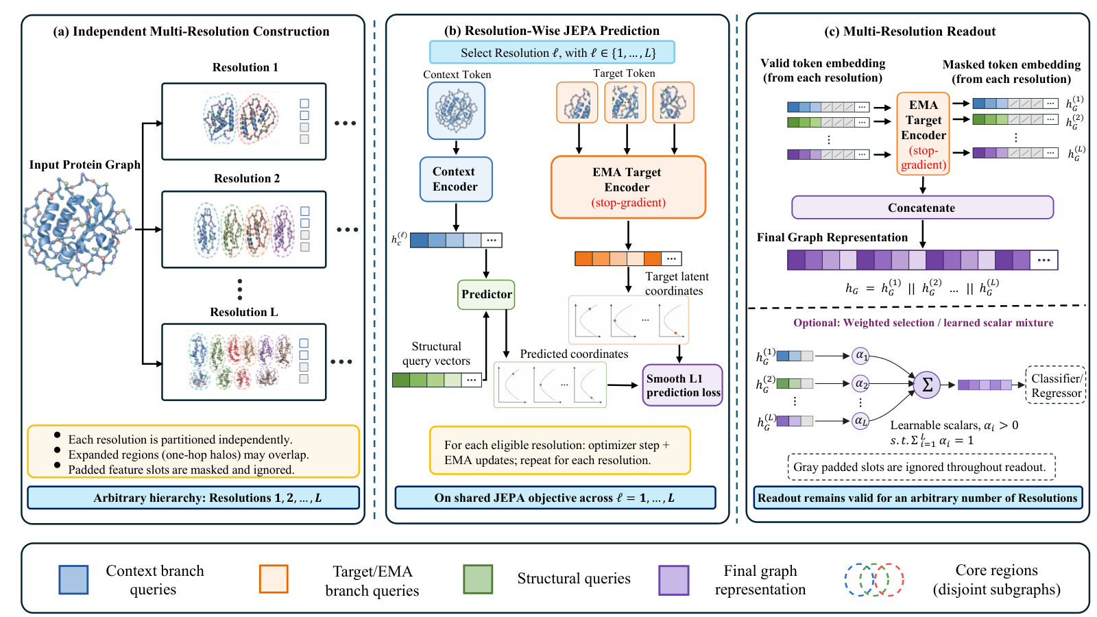
Figure 2. Overview of HP-JEPA.(a) The input graph is partitioned independently at configured resolutions. At resolution , each core region defines a graph-patch support , while padded and inactive token slots are masked and ignored. (b) At each eligible resolution, the sampled context index and target-index set determine the context and target-content inputs processed by the online token encoder and EMA target token encoder , respectively. For each , the predictor estimates from the context state and target structural query , supervised by the two-coordinate target using a coordinate-wise Smooth loss. (c) During downstream readout, the frozen EMA target token encoder processes each active resolution independently, and its valid token representations are mean-pooled to obtain . The resolution-specific representations are subsequently combined through concatenation or uniformly smoothed task-specific resolution weighting for graph classification or regression.HP-JEPA independently constructs graph regions at multiple resolutions, performs two-coordinate latent prediction separately within each eligible resolution, mean-pools valid token representations to obtain resolution-specific graph representations, and combines those representations through concatenation or task-specific resolution weighting.
A context patch and a structural query predict a transformed statistic of a target patch’s representation. The source’s two-coordinate target retains the feature mean through a Lorentz-coordinate map, not the complete latent vector. The appendix characterizes exactly that retained projection. It should not be described as a lossless embedding of every target-feature direction.
4. Method
The method combines independent multi-resolution partitioning, a separate prediction update at each eligible resolution and frozen readout. These three choices are distinct parts of the pipeline.
4.1. Multi-Resolution Graph Tokenization
Each active resolution partitions the full graph independently. Tokens describe patch content and structural context; padding slots are masked, and overly fine resolutions become inactive for small graphs. There is no required nesting between resolutions. Expanded patch supports can overlap even when their core regions form a partition.
4.2. Resolution-Wise Joint-Embedding Prediction
Prediction uses context content plus a target structural query, while the EMA target branch receives detached target content without that query. The loss matches two coordinates of a feature-mean statistic with SmoothL1. Graphs with more selected targets contribute more within the token-normalized batch loss. Resolutions are processed with sequential optimizer updates; no parent–child or cross-resolution consistency term is added.
4.3. Multi-Resolution Readout and Task-Specific Resolution Weighting
After pretraining, each resolution is encoded and pooled independently. Concatenation preserves the separate feature slots; a learned mixture instead uses weights shared across a downstream task and split. That mixture uses downstream labels and is not graph-specific attention. Inactive slots contribute zero and weights are not renormalized per graph. The appendix’s oracle comparison concerns a bounded fixed-feature readout family, not nonlinear pretraining convergence.
Table 2. Results on graph classification and regression benchmarks. For reference only, we include the results of F-GIN, a pioneering end-to-end supervised GNN. SSL methods are grouped by pretraining paradigm in the following order: contrastive, generative, self-predictive, and JEPA. Baseline results are taken directly from prior work (Hassani and Khasahmadi, 2020; Tan et al., 2023; Suresh et al., 2021; Skenderi et al., 2025) and "-" indicates that the corresponding results are not reported. The best SSL result is underlined, and the second best is wavy underlined. For a more direct comparison, HP-JEPA results that outperform the Graph-JEPA baseline are highlighted with a red cell background.
Experiments cover graph classification, molecular regression, a representation case study and sensitivity to graph size and resolution banks. Each probes a different part of the multi-resolution motivation.
5.1. Downstream Task Evaluation
The task evaluation separates the frozen representation from the supervised classifier or regressor trained on it. Data splitting and tuning determine the scope of a fair comparison.
5.1.1. Setup
Seven classification benchmarks use repeated stratified cross-validation; ZINC-12K uses its standard regression split. Baselines include both latent-prediction and generative graph methods. The appendix specifies which preprocessing and fitting steps use only the corresponding training data.
5.1.2. Results and Discussion
HP-JEPA improves over Graph-JEPA on six of eight tasks and performs best on five in the reported comparison. The two IMDB tasks still favor generative methods, consistent with their small graphs and limited attributes. The empirical result is therefore a useful extension, not universal dominance of latent prediction over reconstruction.
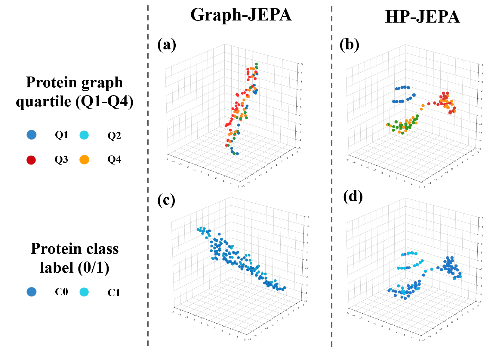
Figure 3. 3D t-SNE visualization of graph-level embeddings on the PROTEINS dataset. Each point represents one protein graph. Columns compare Graph-JEPA and HP-JEPA; the top row colors embeddings by graph-size quartile (Q1–Q4), while the bottom row colors the same embeddings by protein class (C0/C1). Compared with fixed-resolution Graph-JEPA, HP-JEPA produces a more structured representation space, distinctly separating proteins. This alignment indicates that HP-JEPA captures graph-size-dependent structural and functional patterns without using class labels during pretraining.
5.2. Case Study: Learning Multi-Resolution Graph Features
The PROTEINS visualization relates embeddings to labels and graph size. It illustrates structural variation preserved at multiple scales. Size–label association in a benchmark is not evidence that graph size alone supplies a universal biological explanation of enzyme function.
5.3. Sensitivity Analysis
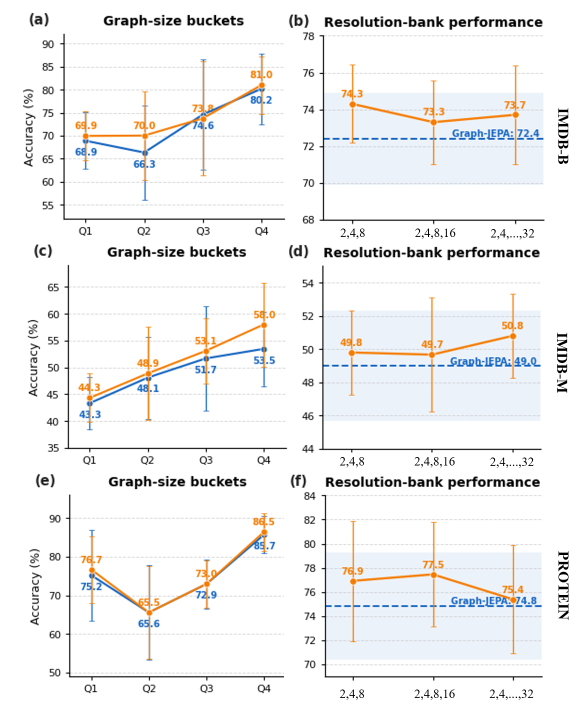
Most size quartiles and all tested resolution-bank settings favor HP-JEPA over the fixed-resolution baseline. The results reduce dependence on choosing one granularity in those datasets, while leaving performance variation across banks visible. They do not establish invariance to every graph-size distribution.
Figure 4. Sensitivity analysis on IMDB-BINARY, IMDB-MULTI, and PROTEINS.
Panels (a), (c), and (e) report Graph-JEPA and HP-JEPA accuracy across node-count quartiles –. Panels (b), (d), and (f) compare HP-JEPA using resolution banks , , and the full bank, with Graph-JEPA shown as a dashed reference. Results are the mean and standard deviation over ten cross-validation folds from one pretrained seed.
6. Conclusion
The contribution is multi-resolution graph representation learning with independent within-resolution prediction and flexible downstream combination. Its gains are benchmark-bounded, and the target geometry preserves a specific statistic rather than the entire latent state.
Appendix A Dataset and Training Details
The appendix documents graph statistics, input features, partitions, splits and task-specific configurations. These details determine what information is available in pretraining and how downstream evaluation avoids leakage.
Table 3. Descriptive statistics of the datasets used in the main experiments. The statistics are adapted from Graph-JEPA (Skenderi et al., 2025). The symbol “–” indicates that ZINC-12K is a graph-regression benchmark and therefore has no discrete class labels.
The configuration fixes capacities, target sampling, optimizer/teacher schedules and downstream choices. The source explicitly distinguishes training-only fitting from held-out evaluation data. Multi-resolution selection and readout tuning must follow those split boundaries.
Table 4. Dataset-specific HP-JEPA pretraining configurations. lists the configured region capacities across resolutions, lists the corresponding numbers of selected target regions, is the random-walk positional-encoding dimension, Drop is module dropout, Tok. is token dropout, and Clip is the maximum gradient norm. All configurations use latent dimension 512 and four Transformer blocks.
Table 5. Dataset-specific downstream readout and linear-probe settings. The readout column reports the mixture of uniform and learned resolution weights, and denotes the recorded regularization parameter of the downstream linear probe.
Appendix B Geometry and Population Characterization of the Latent Target
The geometry result proves that the two-coordinate map preserves distances in the feature-mean projection and is insensitive to components whose mean is zero. It is therefore not injective on the full latent vector. The SmoothL1 population optimum is a conditional Huber location of the target coordinates, not necessarily their conditional mean. The unconstrained predictor is also not guaranteed to output a point on the Lorentz hyperboloid.
Equations 1–4
(1)
(2)
(3)
(4)
Proposition 0 (Geometry and information content of the latent-coordinate map).
For every , the coordinate map in Equation (1) satisfies
Equation 5
(5)
Moreover,
Equation 6
(6)
Consequently,
Equation 7
(7)
Finally,
Equation 8
(8)
where
Equation 9
(9)
Therefore, preserves exactly the feature-mean projection of the target-token state and is invariant to all latent components orthogonal to .
Equations 10–21
(10)
(11)
(12)
(13)
(14)
(15)
(16)
(17)
(18)
(19)
(20)
(21)
Proposition 0 (Population target of coordinate-wise Smooth L1).
For -almost every , suppose that
Equation 22
(22)
Then is convex, coercive, and admits at least one minimizer. A scalar minimizes if and only if
Equation 23
(23)
Thus, the population-optimal coordinate-wise Smooth L1 predictor returns a conditional Huber location functional of the target coordinate.
In particular, let
Equation 24
(24)
If
Equation 25
(25)
then is a minimizer of .
Equations 26–33
(26)
(27)
(28)
(29)
(30)
(31)
(32)
(33)
Appendix C Generalization of Task-Specific Resolution Weighting
The readout bound assumes a pretrained encoder treated as fixed, independent labeled examples, bounded feature/readout norms and an appropriate bounded Lipschitz loss. Within the closed mixture family, approximate empirical risk minimization competes with the best fixed resolution up to complexity and optimization terms. Finite softmax parameters approach simplex vertices only in the closure; uniform smoothing adds an approximation term. These statements do not guarantee convergence of the actual nonconvex pretraining or tuning algorithm.
There exist constants such that the following conditions hold:
Equations 38–41
(38)
(39)
(40)
(41)
Equations 42–44
(42)
(43)
(44)
Theorem 1 (Resolution-adaptive oracle bound).
Under Assumption 1, there exist universal constants such that, for every , with probability at least ,
Equation 45
(45)
Thus, the closed resolution-weighting family competes with the best fixed-resolution linear predictor selected in hindsight, while its additional dependence on the number of configured resolutions is logarithmic in .
Equations 46–66
(46)
(47)
(48)
(49)
(50)
(51)
(52)
(53)
(54)
(55)
(56)
(57)
(58)
(59)
(60)
(61)
(62)
(63)
(64)
(65)
(66)
Lemma 0 (Stability under uniform resolution smoothing).
Gilmer et al. (2017)
Justin Gilmer, Samuel S.
Schoenholz, Patrick F. Riley, Oriol
Vinyals, and George E. Dahl.
2017.
Neural Message Passing for Quantum Chemistry. In
Proceedings of the 34th International Conference on
Machine Learning(Proceedings of Machine Learning
Research, Vol. 70). PMLR,
1263–1272.
https://proceedings.mlr.press/v70/gilmer17a.html
Hamilton et al. (2017b)
William L. Hamilton, Rex
Ying, and Jure Leskovec.
2017b.
Representation Learning on Graphs: Methods and
Applications.
IEEE Data Engineering Bulletin
40, 3 (2017),
52–74.
arXiv:1709.05584
https://arxiv.org/abs/1709.05584
Hassani and Khasahmadi (2020)
Kaveh Hassani and
Amir Hosein Khasahmadi. 2020.
Contrastive Multi-View Representation Learning on
Graphs. In Proceedings of the 37th International
Conference on Machine Learning(Proceedings of
Machine Learning Research, Vol. 119).
PMLR, 4116–4126.
https://proceedings.mlr.press/v119/hassani20a.html
Hou et al. (2022)
Zhenyu Hou, Xiao Liu,
Yukuo Cen, Yuxiao Dong,
Hongxia Yang, Chunjie Wang, and
Jie Tang. 2022.
GraphMAE: Self-Supervised Masked Graph
Autoencoders. In Proceedings of the 28th ACMSIGKDD Conference on Knowledge Discovery and Data Mining.
Association for Computing Machinery,
594–604.
doi:10.1145/3534678.3539321
Huang et al. (2025)
Yongqi Huang, Jitao Zhao,
Dongxiao He, Di Jin,
Yuxiao Huang, and Zhen Wang.
2025.
Does GCL Need a Large Number of Negative Samples?
Enhancing Graph Contrastive Learning with Effective and Efficient Negative
Sampling. In Proceedings of the AAAI Conference on
Artificial Intelligence, Vol. 39.
17511–17518.
doi:10.1609/aaai.v39i16.33925
Kipf and Welling (2017)
Thomas N. Kipf and Max
Welling. 2017.
Semi-Supervised Classification with Graph
Convolutional Networks. In International
Conference on Learning Representations.
arXiv:1609.02907
https://openreview.net/forum?id=SJU4ayYgl
Lei et al. (2025)
Hongyang Lei, Xiaolong
Cheng, Qi Qin, Dan Wang,
Huazhen Huang, Qingqing Gu,
Yetao Wu, and Luo Ji.
2025.
M3-JEPA: Multimodal Alignment via Multi-gate
MoE Based on the Joint-Embedding Predictive Architecture. In
Proceedings of the 42nd International Conference on
Machine Learning(Proceedings of Machine Learning
Research, Vol. 267). PMLR,
33902–33917.
Morris et al. (2020)
Christopher Morris,
Nils M. Kriege, Franka Bause,
Kristian Kersting, Petra Mutzel, and
Marion Neumann. 2020.
TUDataset: A Collection of Benchmark Datasets for
Learning with Graphs.
Computing Research Repository
(2020).
arXiv:2007.08663
https://arxiv.org/abs/2007.08663
Perozzi et al. (2017)
Bryan Perozzi, Vivek
Kulkarni, Haochen Chen, and Steven
Skiena. 2017.
Don’t walk, skip! online learning of multi-scale
network embeddings. In Proceedings of the 2017
IEEE/ACM International Conference on Advances in Social Networks Analysis and
Mining 2017. 258–265.
Qiu et al. (2020)
Jiezhong Qiu, Qibin Chen,
Yuxiao Dong, Jing Zhang,
Hongxia Yang, Ming Ding,
Kuansan Wang, and Jie Tang.
2020.
GCC: Graph Contrastive Coding for Graph Neural
Network Pre-Training. In Proceedings of the 26th
ACMSIGKDD International Conference on Knowledge Discovery and Data Mining.
1150–1160.
doi:10.1145/3394486.3403168
Skenderi et al. (2025)
Geri Skenderi, Hang Li,
Jiliang Tang, and Marco Cristani.
2025.
Graph-Level Representation Learning with
Joint-Embedding Predictive Architectures.
Transactions on Machine Learning Research
(2025).
https://openreview.net/forum?id=v47f4DwYZb
Sun et al. (2020)
Fan-Yun Sun, Jordan
Hoffmann, Vikas Verma, and Jian Tang.
2020.
InfoGraph: Unsupervised and Semi-Supervised
Graph-Level Representation Learning via Mutual Information Maximization. In
International Conference on Learning
Representations.
https://openreview.net/forum?id=r1lfF2NYvH
Tan et al. (2023)
Qiaoyu Tan, Ninghao Liu,
Xiao Huang, Soo-Hyun Choi,
Li Li, Rui Chen, and
Xia Hu. 2023.
S2GAE: Self-Supervised Graph Autoencoders Are
Generalizable Learners with Graph Masking. In
Proceedings of the Sixteenth ACM International
Conference on Web Search and Data Mining. Association
for Computing Machinery, 787–795.
doi:10.1145/3539597.3570404
Thakoor et al. (2022)
Shantanu Thakoor, Corentin
Tallec, Mohammad Gheshlaghi Azar, Mehdi
Azabou, Eva L. Dyer, Rémi Munos,
Petar Veličković, and Michal
Valko. 2022.
Large-Scale Representation Learning on Graphs via
Bootstrapping. In International Conference on
Learning Representations.
https://openreview.net/forum?id=0UXT6PpRpW
Veličković et al. (2019)
Petar Veličković,
William Fedus, William L. Hamilton,
Pietro Liò, Yoshua Bengio, and
R. Devon Hjelm. 2019.
Deep Graph Infomax. In
International Conference on Learning
Representations.
arXiv:1809.10341
https://iclr.cc/virtual/2019/poster/782
Wen et al. (2024)
Qianlong Wen, Mingxuan
Ju, Zhongyu Ouyang, Chuxu Zhang, and
Yanfang Ye. 2024.
From coarse to fine: enable comprehensive graph
self-supervised learning with multi-granular semantic ensemble. In
Forty-first International Conference on Machine
Learning.
Wu et al. (2021)
Zonghan Wu, Shirui Pan,
Fengwen Chen, Guodong Long,
Chengqi Zhang, and Philip S. Yu.
2021.
A Comprehensive Survey on Graph Neural Networks.
IEEE Transactions on Neural Networks and
Learning Systems 32, 1
(2021), 4–24.
doi:10.1109/TNNLS.2020.2978386
Xie et al. (2022)
Yaochen Xie, Zhao Xu,
and Shuiwang Ji. 2022.
Self-Supervised Representation Learning via Latent
Graph Prediction. In Proceedings of the 39th
International Conference on Machine Learning(Proceedings of Machine Learning Research,
Vol. 162). PMLR,
24460–24477.
https://proceedings.mlr.press/v162/xie22e.html
Xu et al. (2019)
Keyulu Xu, Weihua Hu,
Jure Leskovec, and Stefanie Jegelka.
2019.
How Powerful Are Graph Neural Networks?. In
International Conference on Learning
Representations.
arXiv:1810.00826
https://openreview.net/forum?id=ryGs6iA5Km
Zhao et al. (2025)
Songwei Zhao, Yuan Jiang,
Zijing Zhang, Yang Yu, and
Hechang Chen. 2025.
Grain: Multi-granular and implicit information
aggregation graph neural network for heterophilous graphs. In
Proceedings of the AAAI Conference on Artificial
Intelligence, Vol. 39. 13383–13391.