Overview
The paper studies compositional generalization and data-efficient imitation learning through controlled instruction-coverage experiments.
At a glance
The study asks which instruction combinations a robot policy needs to see during training. A bounded-loss distribution-shift analysis distinguishes factor marginals, instruction recombinations, and conditional context/action changes. Simulated manipulation experiments show that pair-covering task subsets can match full enumeration at a fixed demonstration budget, while sparse pretrained policies can benefit from small amounts of broader supervision. Dependent tasks require preserving cross-stage information. The results concern a small controlled task family and do not provide a universal coverage rule for pretrained robot models.
1 Introduction
A policy may observe every object, container, and button individually yet fail when they appear in a new combination. The paper treats instruction coverage as a dataset-design variable, comparing sparse correlated task sets with structured subsets that cover factor pairs. It also separates recovering already learned behaviors under new instructions from learning entirely new manipulation skills. The proposed principle is to cover action-relevant dependencies, with the required interaction order depending on the task.
2 Related Work
The related work connects instruction-conditioned policies, compositional benchmarks, experimental design, and hierarchical control.
Language-Conditioned Robot Policies.
Generalist robot policies can map language or multimodal prompts to actions, but scaling a policy does not specify which combinations its demonstrations must cover. This paper isolates instruction-tuple coverage in a common flow-matching architecture rather than proposing a new large pretrained robot policy.
Compositional Generalization in Language and Robotics.
Compositional benchmarks hold out recombinations of familiar factors. In robotics, changing those combinations also changes the observations reached and the appropriate actions. The analysis therefore includes conditional context/action shift in addition to changes in the instruction distribution.
Data Coverage and Combinatorial Designs.
Data-generation approaches such as MimicGen [17] increase demonstrations, while orthogonal designs [12] motivate covering interactions without enumerating every tuple. The experiments use this design idea to compare task breadth with the number of demonstrations per selected task.
Modularity and Hierarchy.
Hierarchical policies can expose only the active subtask, reducing dependence on irrelevant instruction components. This helps when stages are independent, but can discard information needed for cross-stage constraints. The idealized modular comparison assumes a correct stage indicator, whose construction is explicitly documented.
3 Problem Statement
An instruction is an ordered tuple of discrete subtask values. A conditional policy maps the current observation/state and instruction tuple to an action distribution. A stage indicator identifies the currently active subtask. The task family is designed so individual factor values are familiar while selected combinations are withheld.
3.1 Compositional Generalization Gap
Training and test joint distributions include instructions, contexts, and actions. Held-out instructions are valid tuples absent from the selected training support. The formal generalization gap is the difference in expected policy loss, instantiated experimentally with flow-matching loss. This loss gap is distinct from the measured difference in rollout success.
Equations 1–4
| (1) | ||||
| (2) |
| (3) |
| (4) |
4 Theoretical Analysis
The proposition bounds the absolute risk gap by a loss bound times three L1 distribution discrepancies: active-factor marginals, the remaining instruction factors conditional on that factor, and context/action distributions conditional on the complete instruction. The proof is a distribution-factorization and triangle-inequality argument.
The result assumes a uniformly bounded loss. It is a diagnostic decomposition, not a finite-sample guarantee that pairwise task coverage suffices. Matching low-order pairs need not match the full instruction-tuple distribution, and merely observing every factor value does not ensure matching marginal frequencies. The experiments, rather than the bound alone, establish the usefulness of the chosen designs in these tasks.
Equations

4.1 Stage-wise Modular Policy
A stage-wise controller receives the current context and only the active instruction. Under bounded stage losses, integrating out inactive instruction factors removes the explicit full-instruction composition term from the bound. Their influence can still remain through context/action distributions. If the correct current action depends on an omitted future instruction, the modular input is insufficient even with an oracle stage indicator.
Equations

5 Experiments
The experiments test whether exhaustive tuple coverage is necessary, what sparse-pretraining failures reflect, and what coverage is required when one instruction factor constrains another stage’s actions.

5.1 Experimental Setup
All main tasks are simulated sequential manipulation problems with controlled discrete factors, generated demonstrations, a common policy architecture, and held-out combinations.
Task Design.
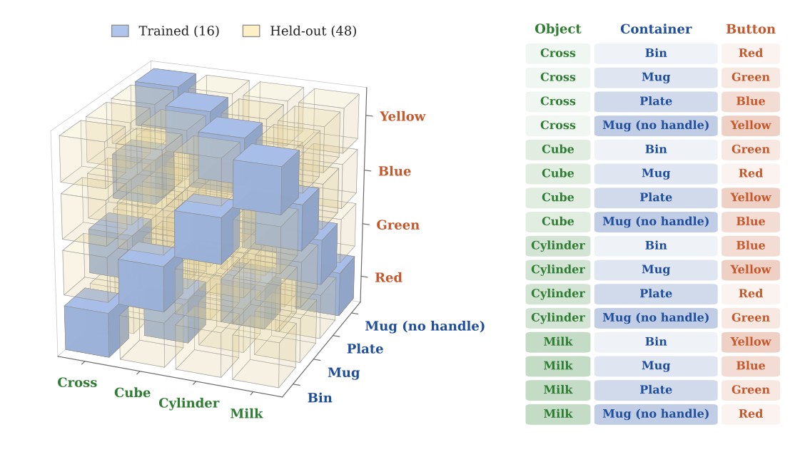
Pick-and-Place has four objects and four containers, giving sixteen tasks. Pick-Place-Press adds four buttons, giving 64 tuples. Two-Stage Pick-and-Place uses different objects and different containers across the two placements, giving 144 fully specified combinations. Its policy input omits the first container and contains only the two objects and final container: this leaves 48 instruction tuples, each with three valid first-container choices. The first placement must therefore account for a later instruction while remaining multimodal.
Data and Policy.
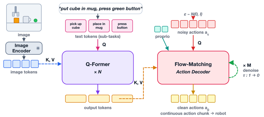
A customized motion planner supplies demonstrations. Policies use a frozen DINOv2 [21] image encoder and a transformer flow-matching action model trained from scratch. Across different numbers of selected training tasks, total demonstration count is fixed and allocated uniformly among those tasks. Fewer selected tasks consequently receive more examples per task.
Evaluation Protocol.
Success is reported over all tasks, selected training tasks, and held-out instruction tuples. The full-task baseline has no held-out tuples; its overall success is repeated in the plots only as a reference. Most experiments use three training seeds and thirty rollouts per task. Same-container violation rate is conditional on completing the first placement, excluding earlier failures, so it must be read alongside success rate.
5.2 Q1: Is Full Tuple Coverage Necessary?
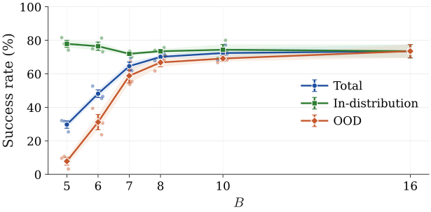
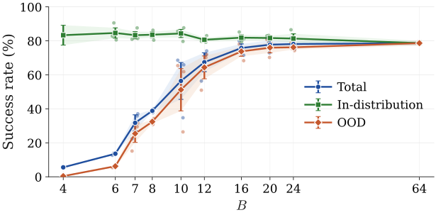
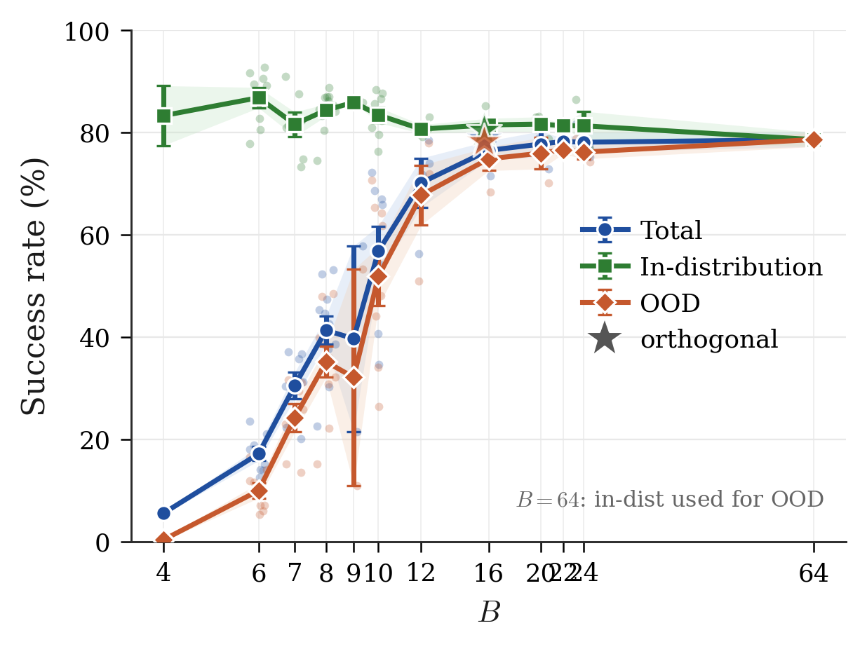
Small task sets perform poorly on held-out tuples even when every individual instruction value appears. Performance saturates near eight of sixteen Pick-and-Place tasks and sixteen of 64 Pick-Place-Press tasks. For three PPP training sizes, held-out flow loss falls from 0.03421 to 0.01548 to 0.00756 while held-out success rises from 0.83% to 23.93% to 82.29%; training losses remain similar.
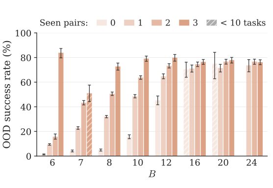
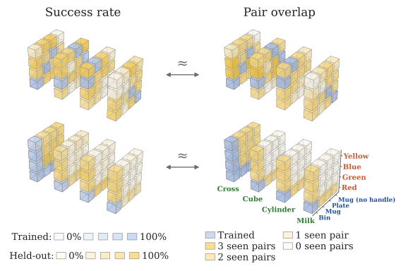
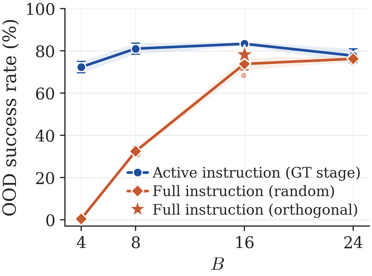
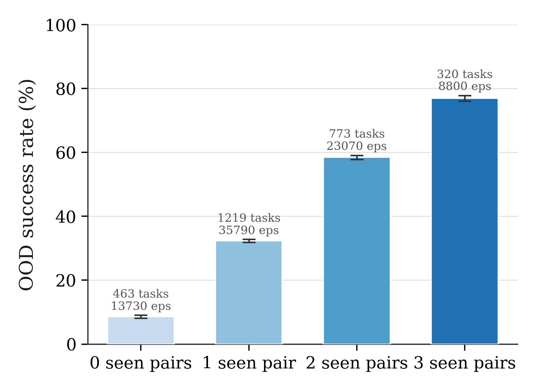
Within a fixed budget, tasks whose object–container, object–button, and container–button pairs have been seen tend to perform better. A sixteen-task orthogonal design covers every pair exactly once and achieves 78.2% held-out success, close to the 78.6% overall success of full-task training. This supports pair coverage in this independent three-factor task, without proving that pair coverage is sufficient for longer or more dependent tasks.
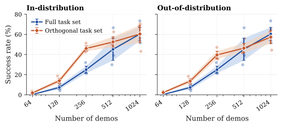
Fixed-budget comparison.
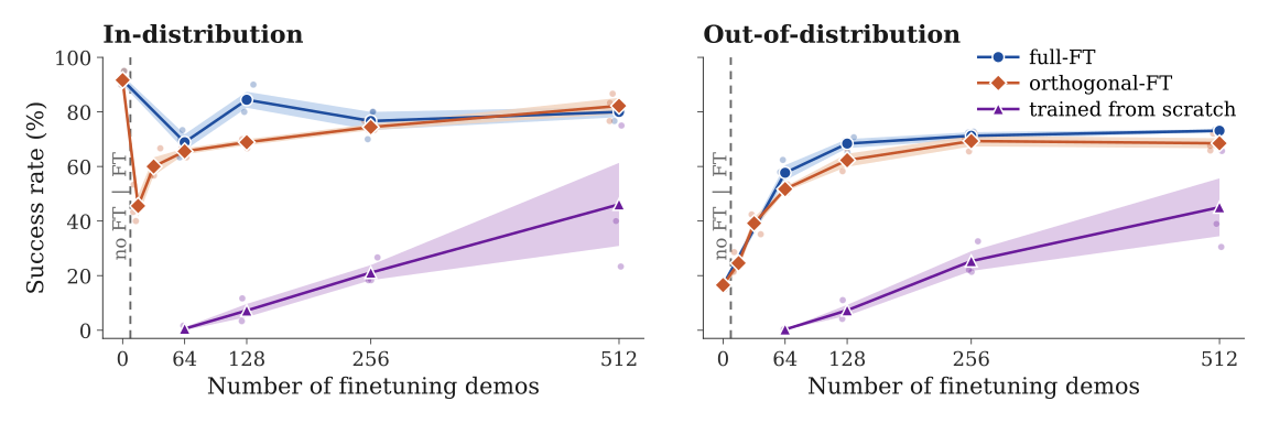
At low and medium total demonstration budgets, the orthogonal subset outperforms full enumeration. Concentrating data on fewer structurally informative tasks provides more examples per selected tuple. The gap narrows with larger budgets. This comparison tests allocation at a fixed total data count, not a claim that reducing both tasks and demonstrations always improves performance.
5.3 Q2: What Is Missing When Sparse Coverage Fails?
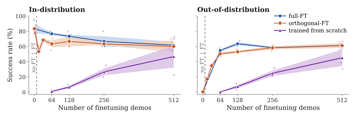
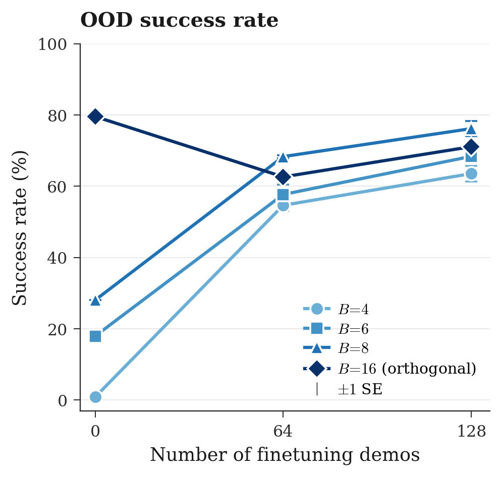
A diagonal four-task set ties each object, container, and button together. It yields high training success but only 0.4% success on the originally unseen combinations. Finetuning with one demonstration for each of all 64 tasks raises that group’s success to 54.7%, substantially more than learning from the small broader dataset alone.
Those formerly held-out tuples are now represented in the finetuning data. The 54.7% figure therefore measures adaptation to combinations unseen during pretraining, not final-model zero-shot success on tuples withheld from every training phase. The result supports reusable learned skills but does not uniquely isolate instruction routing as the causal failure mechanism.
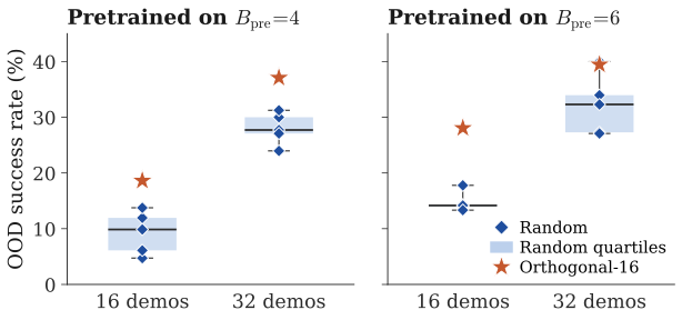
Separate matched-budget comparisons favor orthogonal over random finetuning task selection for sparse pretrained checkpoints. Training-task success can decrease, and strong pretrained policies can worsen after tiny finetuning sets, exposing reweighting and overfitting tradeoffs.
5.4 Q3: What Coverage Is Needed for Dependent Instructions?
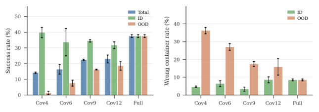
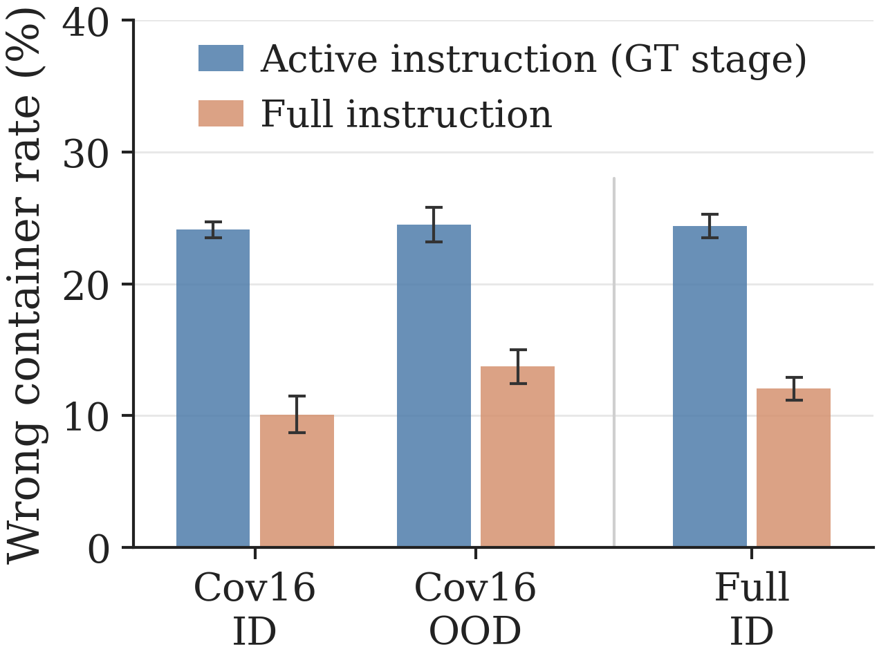
For the dependent task, vary coverage of the first-object/final-container pair while fixing the number of selected training tuples. In the 36-instruction version, twelve training tasks cover twelve, nine, six, or four such pairs. Broader pair coverage improves held-out success and reduces same-container violations; narrower coverage can improve in-distribution performance by concentrating supervision. The relevant pairs are known from the task design rather than automatically discovered by the method.
Comparison with stage-wise modular policies.
Oracle stage selection helps the independent PPP task under sparse coverage. In the dependent task, the modular controller receives only the first object during the first placement and cannot condition on the forbidden final container. A full-instruction controller retains that information and reduces held-out container violations with broader dependent-pair coverage. This comparison exposes a deliberate information bottleneck in the specified modular input, not a general failure of all hierarchical policies.
6 Conclusion and Limitations
The evidence favors structured coverage of action-relevant instruction interactions over automatic full enumeration in these controlled tasks. Limitations include the small simulated task family, known dependency structure, combinatorial evaluation cost, and policies trained from scratch over frozen vision features. The analysis assumes bounded losses and does not estimate a universally sufficient interaction order. Transfer to large pretrained vision–language–action models remains future work.
Acknowledgments
The study acknowledges support from FANUC.
Appendix A Theoretical Analysis
The general proof factors the joint density into an active instruction marginal, the remaining-instruction conditional, and a context/action conditional. Adding and subtracting two intermediate products separates the density difference into three terms. Integrating against a bounded loss and applying the triangle inequality gives the stated bound.
The modular proof expands risk by stage, uses the stage indicator, and integrates away inactive instructions because each stage loss depends only on the current factor. A second density decomposition yields marginal and conditional-context terms for each stage. This algebra explains the simplified bound but does not remove information required by dependent actions or establish a nontrivial numerical guarantee for the empirical flow loss.
Equations 8–9

| (8) | ||||
| (9) |

Appendix B Experimental Details
The supplementary protocol separates generated demonstration pools from the smaller budgets actually selected for each experiment and documents architecture, evaluation, and exceptions.
B.1 Data Generation and Training Protocol
Generated pools contain 500 demonstrations per PP task, 300 per PPP task, and 100 per fully specified 2S-PP task: 8,000, 19,200, and 14,400 demonstrations. Experiments select subsets under their stated budgets; they do not necessarily use the full pool. PPP trains for 100,000 steps at batch size 64, and dependent 2S-PP for 150,000 steps. Seeds vary demonstration selection and initialization.
B.2 Policy Architecture
Inputs include third-person and wrist images plus robot state, including gripper pose. Instruction tokens query image tokens in a Q-Former-style interaction and condition a flow transformer through cross-attention. Actions specify end-effector position/orientation deltas and gripper actuation. The vision encoder is frozen across these experiments.
B.3 Evaluation Protocol
Metrics are computed per training seed and then averaged. Full-task curves display overall success in both training and held-out panels because no unseen instruction remains. The 48-instruction dependent experiments instead use five seeds and ten rollouts per task. Conditional violation rates omit trajectories that fail before the first placement and can therefore conceal differences in earlier-stage failures.
Sensitivity to evaluation trial count.
Increasing evaluation from fifteen to thirty rollouts per task changes training and held-out success by 1.04 and 0.41 percentage points in the listed sensitivity example. This supports the selected trial count for that setting but is not a general statistical confidence bound for every comparison.
Appendix C Q1: Is Full Tuple Coverage Necessary?
Additional PPP experiments expand the task-subset sweep and include a separate simulation experiment with human demonstrations.
Pick-Place-Press.
Fifty-five PPP training-set configurations reproduce the broad relationship between more informative pair coverage and held-out success. The complete figure retains both the training-size trend and held-out performance grouped by seen-pair count.
Human demonstrations.
A separate Isaac Lab task has three objects, containers, and target stations, giving 27 combinations. Human SpaceMouse demonstrations supply thirty examples per task, and the policy trains on a nine-task orthogonal subset. Across three seeds and thirty trials per task, training success is 11.67% and held-out success 12.96%. The similar rates suggest limited compositional degradation, but the low absolute success prevents interpreting this as strong manipulation performance or a physical-robot demonstration.
Appendix D Q2: What Is Missing When Sparse Coverage Fails?
Finetuning lasts 5,000 steps after 100,000 pretraining steps, both at batch size 64. Six-task pretraining shows similar adaptation benefits, and stronger pretrained checkpoints usually yield better final performance. However, an already strong sixteen-task orthogonal checkpoint can degrade when finetuned on just 64 broader demonstrations, consistent with overfitting and a shift in task weighting. The full finetuning curves preserve both training and formerly held-out performance.
Appendix E Q3: What Coverage Is Needed for Dependent Instructions?
Dependent-task policies train for 150,000 steps. The supplement gives failure-stage breakdowns, the expanded 48-instruction design, oracle tracking rules, and an experiment isolating ambiguous container choice.
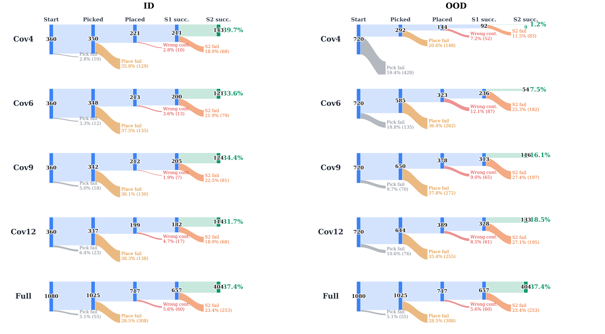
36-task set.
The 36-instruction failure diagrams show that low dependent-pair coverage harms not only container choice but also grasping. Moving from four to six covered pairs reduces some early failures, while wrong-container placement remains common. These breakdowns show why a violation rate conditioned on successful first placement is insufficient by itself.
48-task set.
Allowing four final-container choices gives 48 partial instruction tuples. Sixteen selected training tasks cover sixteen, twelve, nine, or six dependent pairs, with five training seeds and ten evaluation trials per tuple. Broader coverage again improves held-out success and container separation, while narrower coverage concentrates supervision and can improve training-task metrics.
Ground-truth stage indicator.
The oracle tracker uses robot, object, and container state to detect grasps and valid placements, requiring two consecutive matching observations and permitting reversal if progress is lost. PPP exposes object, container, then button instructions. The dependent task exposes first object, second object, then final container.
The tracker uses the final-container constraint to validate the first placement, but the low-level modular controller does not receive that container during the first stage. Tracking poses are not added as policy inputs, and episode success is checked separately. This preserves the distinction between privileged stage supervision and the information available for action selection.
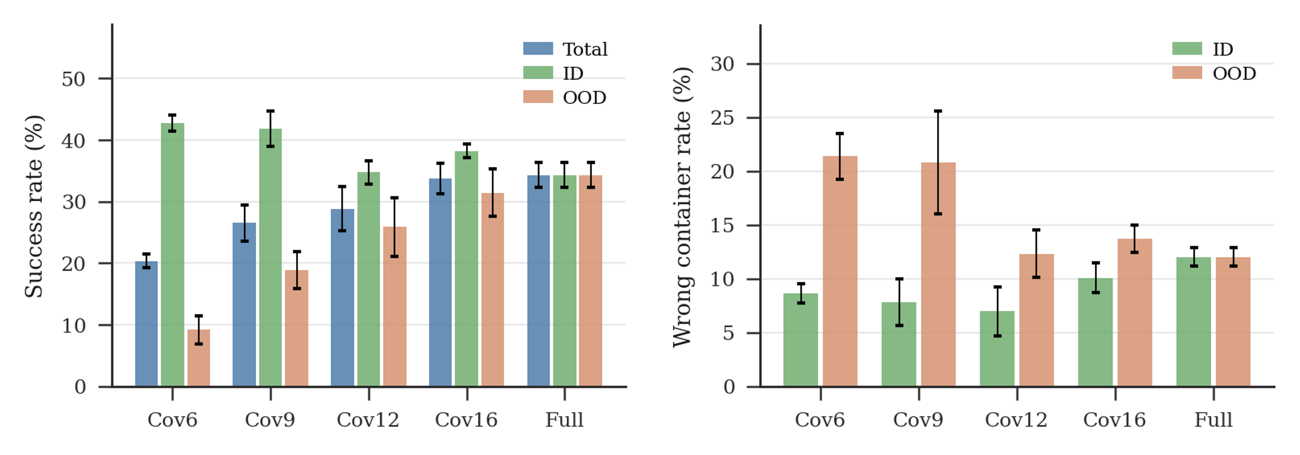
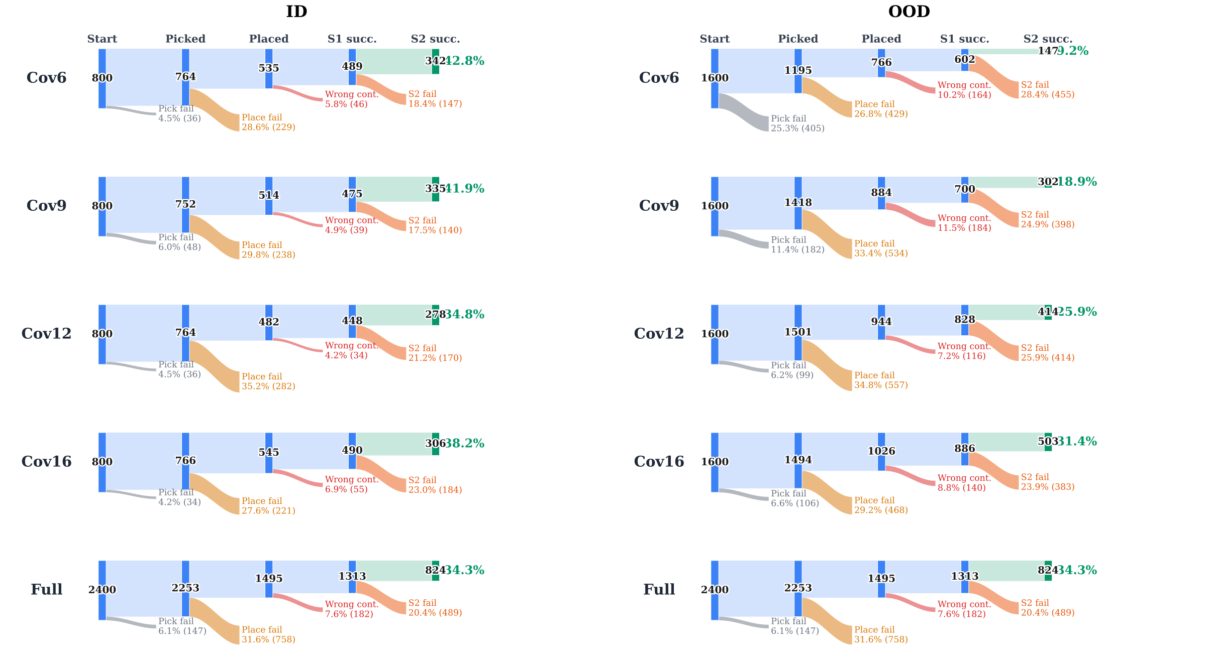
Factors limiting task success in 2S-PP.
Omitting the first-container label leaves several valid placement modes. In an auxiliary PP experiment over five seeds, removing the container instruction lowers success from 71.05% ± 5.00% to 49.95% ± 1.14%. This supports multimodal ambiguity as another difficulty beyond pair coverage. Sequential grasp-and-place errors also accumulate; improved learning from these demonstrations is left open.