Overview
Intuition: pressing piano keys and the sustain pedal changes the sound that follows. Music-JEPA learns that relationship using synchronized recordings and performance controls. It is trained offline from audio–MIDI pairs, not by physically interacting with a piano and not from unlabeled audio alone. Its planning application uses a learned inverse predictor to infer actions rather than an unrestricted successful online search procedure.
At a glance
Music-JEPA treats a short audio segment as a state and its aligned pianoroll/pedal signal as an action. It predicts future latent audio under those controls and learns a temporal prior over actions. Frozen audio features support music tasks, and an additional inverse predictor and decoder support transcription. Evidence is specialized to classical piano and the supplied synchronized performance data.
1 Introduction
A passive audio encoder can learn musical similarity without learning how a control changes future sound. The paper adds performance actions to the predictive problem. This makes piano a useful bounded test case because aligned MIDI supplies pitch, velocity and pedal information. The supervision includes those control streams even though JEPA predicts latent features rather than waveform samples.
2 Related Works
The related work contrasts general music encoders, audio-only joint embeddings, transcription and latent world models. The action-conditioned contribution should be separated from broad music-understanding claims: the experiment uses a particular instrument and a particular paired dataset.
3 Method
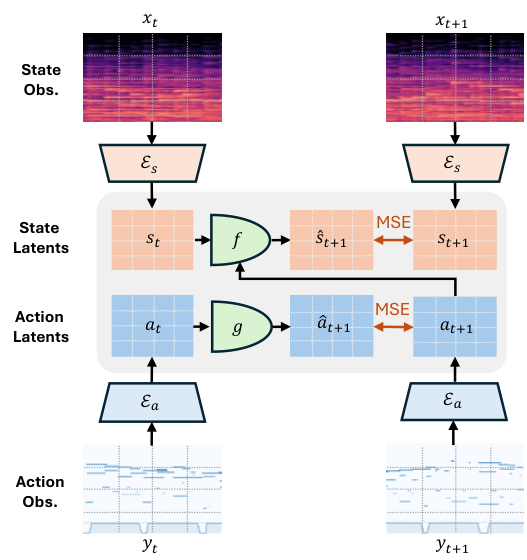
The state predictor maps current audio and an aligned next action toward the next audio state. A separate action predictor supplies a temporal prior. Because controls are aligned with the segment they produce, the source’s action index differs from another common state-transition convention.
Equation 1
| (1) |
3.1 Data Representation
Two-second audio windows become log-mel spectrograms. Aligned MIDI becomes a time-by-pitch pianoroll with note velocity plus a sustain-pedal sequence. These controls are observed in training; inferring them from audio is a later downstream task.
3.2 Model Architecture
Transformer encoders process image-like patches of spectrograms and pianorolls. Pedal features are fused with note-action tokens. The state predictor uses cross-attention to action features, whereas the action predictor models their temporal progression. The architecture diagram and source equations retain the exact masking and indexing.
Equation 2
| (2) |
3.3 Training Objective and Regularization
The loss combines next-audio-feature prediction and an action-feature prior. Stop-gradient moving-average teachers and layer normalization control target dynamics and feature scale. These are the implemented anti-collapse precautions, not a general theorem guaranteeing informative representations under every training condition.
Equations 3–4
| (3) |
| (4) |
3.4 Downstream Tasks and Planning
Frozen state features feed supervised downstream probes. Transcription is posed as choosing actions that explain a desired audio sequence, but high-dimensional direct optimization is unstable. The implemented solution trains an inverse predictor and action decoder while freezing JEPA. This is amortized inverse inference rather than a demonstrated general-purpose online planner.
Equation 5
| (5) |
4 Experiments
Evaluation separates transition sensitivity, representation utility and transcription. A successful metric in one of these settings does not automatically establish the others.
4.1 Dataset and Training Details
Training uses the approximately 200-hour MAESTRO classical-piano collection with synchronized MIDI and its standard splits. The roughly 19 million-parameter system is trained on one A 100. Its domain and action format are substantially narrower than those of a general audio foundation model.
4.2 Baseline Models
An audio-only JEPA is reimplemented on the same piano dataset to test the value of action conditioning. MERT supplies a broader pretrained reference, with different scale and training data. The authors explicitly avoid claiming general superiority over MERT.
| Model | Input State | Target State | ||
| Temporal | Random | Temporal | Random | |
| Ours | 0.929 | 0.999 | 0.991 | 0.992 |
| AO-JEPA | 0.787 | 0.986 | 0.576 | 0.984 |
| Model | Encoder Params. | Beat Tracking | Composer Identification | Key Recognition | ||||||||||
| P70 | R70 | F170 | P100 | R100 | F1100 | wF1 | Top-1 | Top-3 | Top-5 | wP | wR | wF1 | ||
| Ours | 6M | 0.5346 | 0.8159 | 0.6208 | 0.5695 | 0.8634 | 0.6599 | 0.5520 | 0.3540 | 0.7045 | 0.8734 | 0.7638 | 0.7625 | 0.7617 |
| AO-JEPA | 6M | 0.4929 | 0.8506 | 0.6013 | 0.5185 | 0.8941 | 0.6325 | 0.4606 | 0.3308 | 0.6635 | 0.8422 | 0.7657 | 0.7625 | 0.7615 |
| MERT | 95M | 0.4932 | 0.7368 | 0.5780 | 0.5379 | 0.8040 | 0.6309 | 0.6690 | 0.4059 | 0.6493 | 0.7996 | 0.6580 | 0.6485 | 0.6469 |
4.3 Evaluation of Latent Dynamics
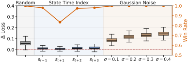
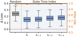
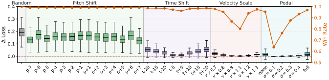
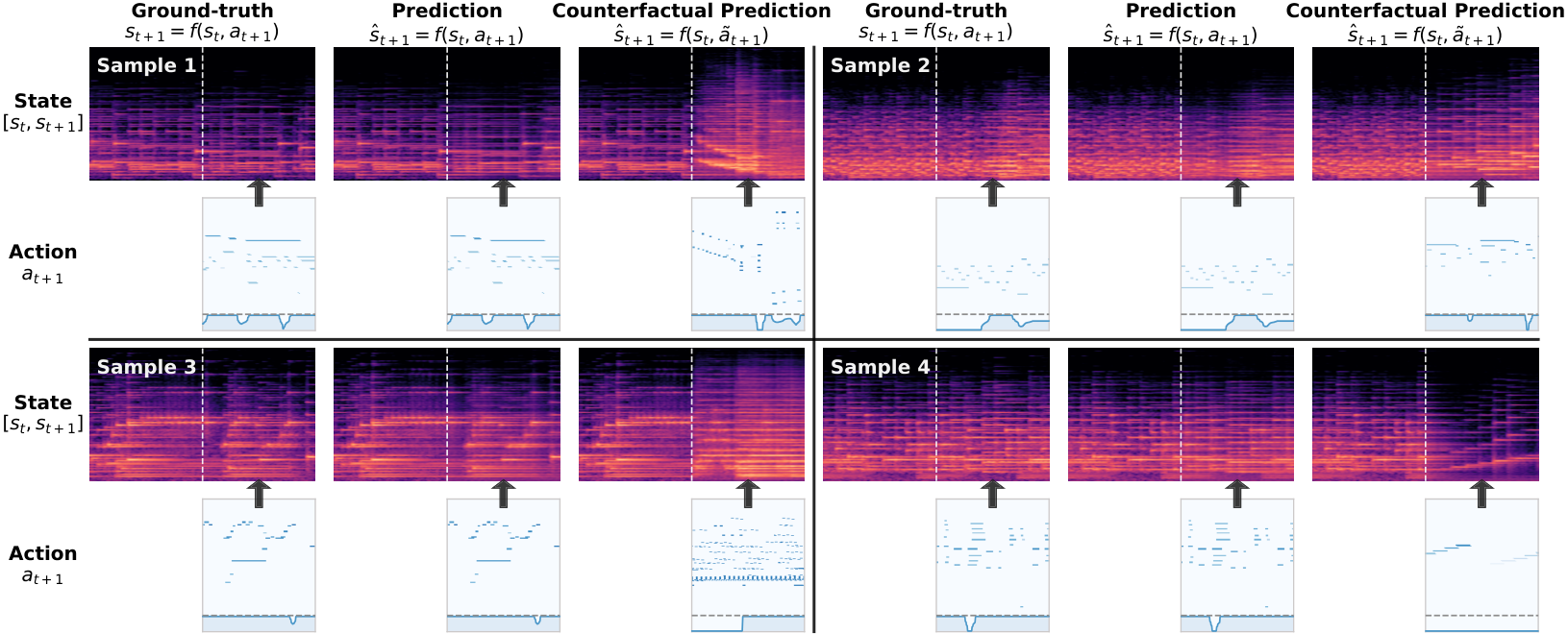
Correct state–action–target triplets should receive lower latent error than deliberately mismatched ones. Temporal, pitch, velocity and pedal perturbations test that sensitivity. The win rate counts how often a perturbation raises loss; it is not a musical-quality or long-horizon planning success rate. A separately trained spectrogram decoder illustrates counterfactual responses to changed actions.
Equation 6
| (6) |
4.4 Evaluation on MIR Downstream Tasks
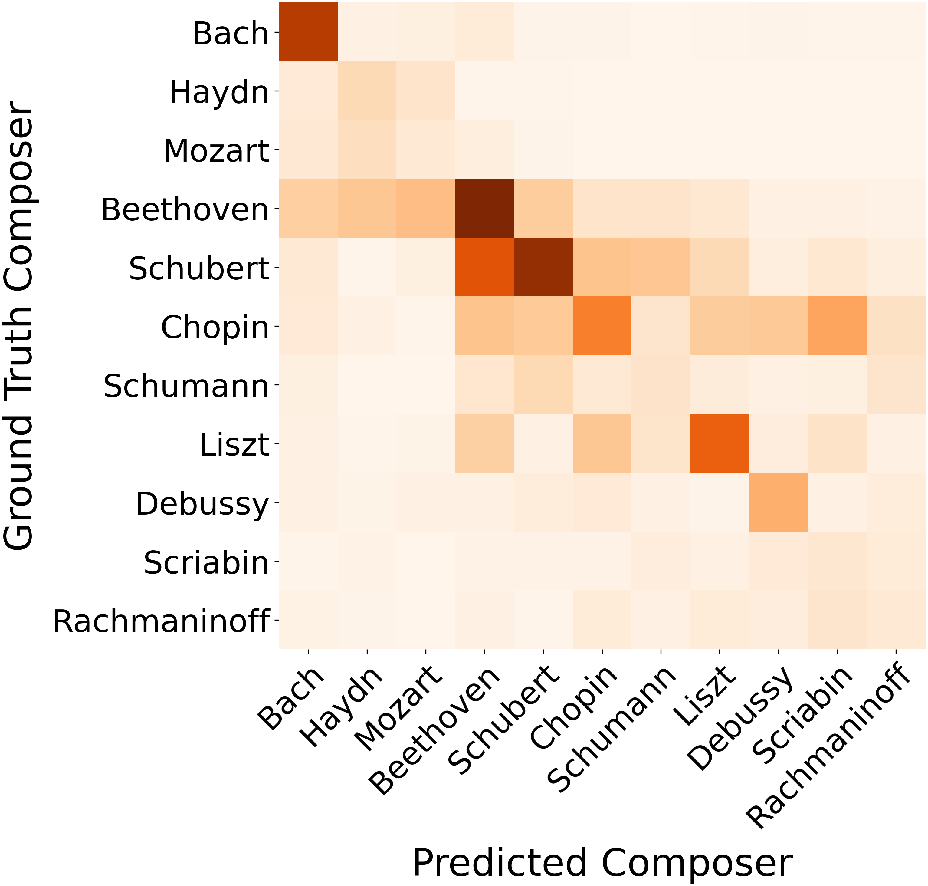
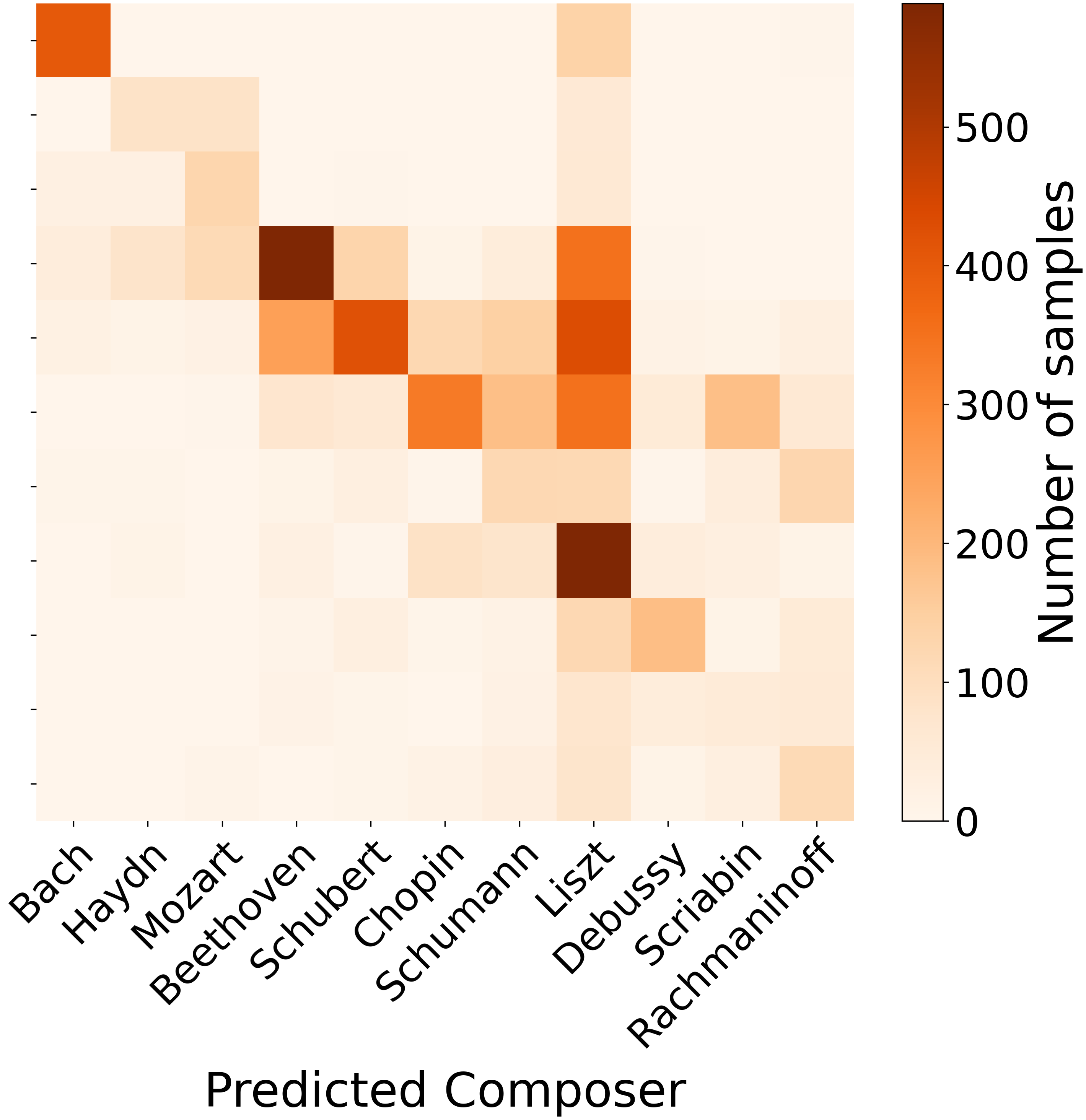
Frozen-feature probes test beat tracking, composer identity and key recognition. Music-JEPA improves over the matched audio-only model and remains competitive with the larger general encoder in these piano tasks. The supervised probe heads, clip lengths and tolerances differ across tasks, so results do not establish zero-shot music understanding.
4.5 Transcription via Planning
The inverse predictor produces latent actions and a separate decoder converts them into pianoroll and pedal outputs. Note-level transcription remains below the fully supervised methods compared, while continuous pedal estimation is stronger in the reported metric. The favorable pedal result and coherent examples should not obscure the weaker note accuracy.
| Model | Note F1 | Pedal | |||
| Frm. | Ons. | +Off. | +Vel. | MAE | |
| Ours | 0.8381 | 0.7325 | 0.5372 | 0.4000 | 0.1222 |
| Kong et al. [41] | 0.9113 | 0.9681 | 0.8524 | 0.8377 | 0.1471 |
| Yan et al. [42] | 0.9375 | 0.9833 | 0.9166 | 0.9122 | 0.1414 |
| Zhang et al. [16] | — | — | — | — | 0.1339 |
5 Conclusion and Future Work
The work demonstrates useful action-conditioned piano representations and an exploratory inverse-inference application. Broader instruments, sound environments and more reliable high-dimensional planning remain future directions. The offline paired-control setup is part of the result’s scope.