Overview
Revisable sequence generation through token-wise noise schedules, with all original diagrams, numerical results and appendix material retained.
At a glance
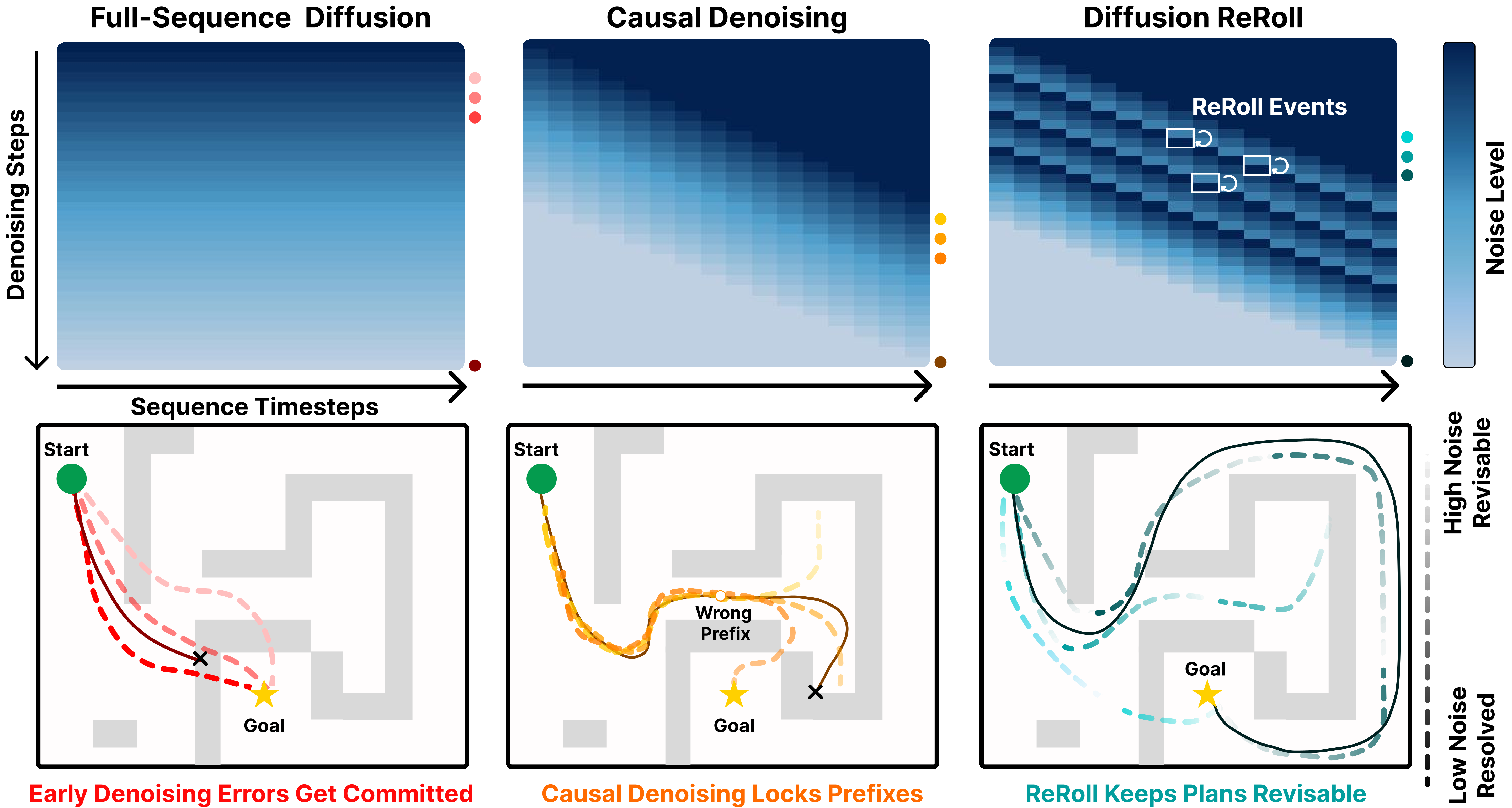
Diffusion ReRoll repeatedly re-noises selected trajectory regions while other regions continue denoising, allowing updated distant context to revise earlier predictions. Randomized piecewise-linear noise profiles train the model for these schedules. Tests span maze planning, manipulation, joint video/action generation and physical navigation. The headline gains are relative improvements in success, not percentage-point differences; benefits depend on aligned training, schedule choices and evaluation protocol.
1 Introduction
Standard diffusion denoises a whole sequence monotonically; Diffusion Forcing assigns individual token noise levels and can resolve a sequence causally. ReRoll keeps regions revisable through structured noise resets and full attention, so early commitments can change when later context improves. It combines randomized linear-chunk training with programmable forward or bidirectional schedules, without adding a separate repair model. Across matched maze protocols, mean success rises 72.8→88.1% over Diffusion Forcing with guidance and 73.8→90.8% over Diffuser with goal inpainting. LIBERO’s official-reset mean rises 40.1→62.7% over Diffusion Policy, averaged across several horizons/history lengths. These empirical comparisons do not establish a universal advantage or isolate every architectural difference.
2 Preliminaries
The method builds on conditional diffusion and token-specific noise levels. Sequence position and diffusion index are distinct axes of the schedule matrix.
2.1 Generative Sequential Prediction
Predict action, state or video-latent tokens from observations, goals or rewards. Subscripts index sequence time; superscripts index diffusion noise. Level zero is clean and K is the Gaussian endpoint. “Noise level” denotes the discrete index, rather than physical variance or SNR. The original forward-corruption equation and cumulative variance schedule remain available.
Equation 1
| (1) |
2.2 Per-Token Noise Levels and Diffusion Forcing
A schedule matrix records each token’s noise level at every sampling step. Fully noisy tokens are effectively masked; clean tokens expose information; intermediate levels provide partial context. Diffusion Forcing trains with independently sampled token levels, enabling causal schedules. ReRoll retains this interface but changes the distribution of training profiles and introduces nonmonotonic sampling.
Equation 2
| (2) |
3 Diffusion ReRoll
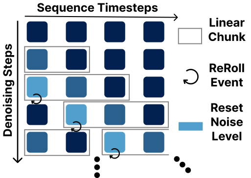
Virtual linear chunks are piecewise-linear noise profiles over one sequence, not separately generated trajectory segments. When a chunk edge reaches a reset threshold, its region returns to full noise and joins a neighboring wave. Full-attention Transformers then revise it using the rest of the horizon. The backbone only needs per-token noise conditioning; patches of one video-latent frame share a level.
3.1 Schedule Matrix for Diffusion ReRoll
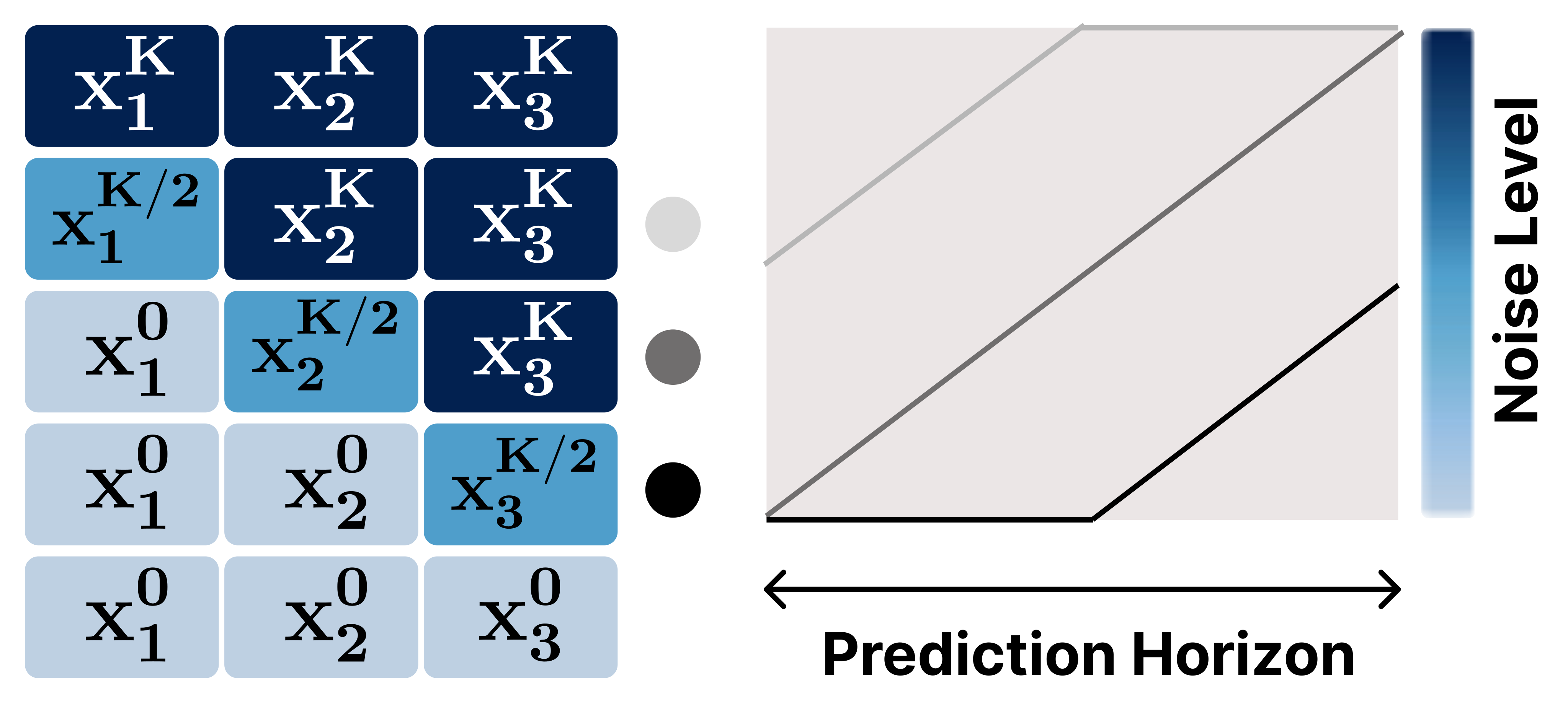
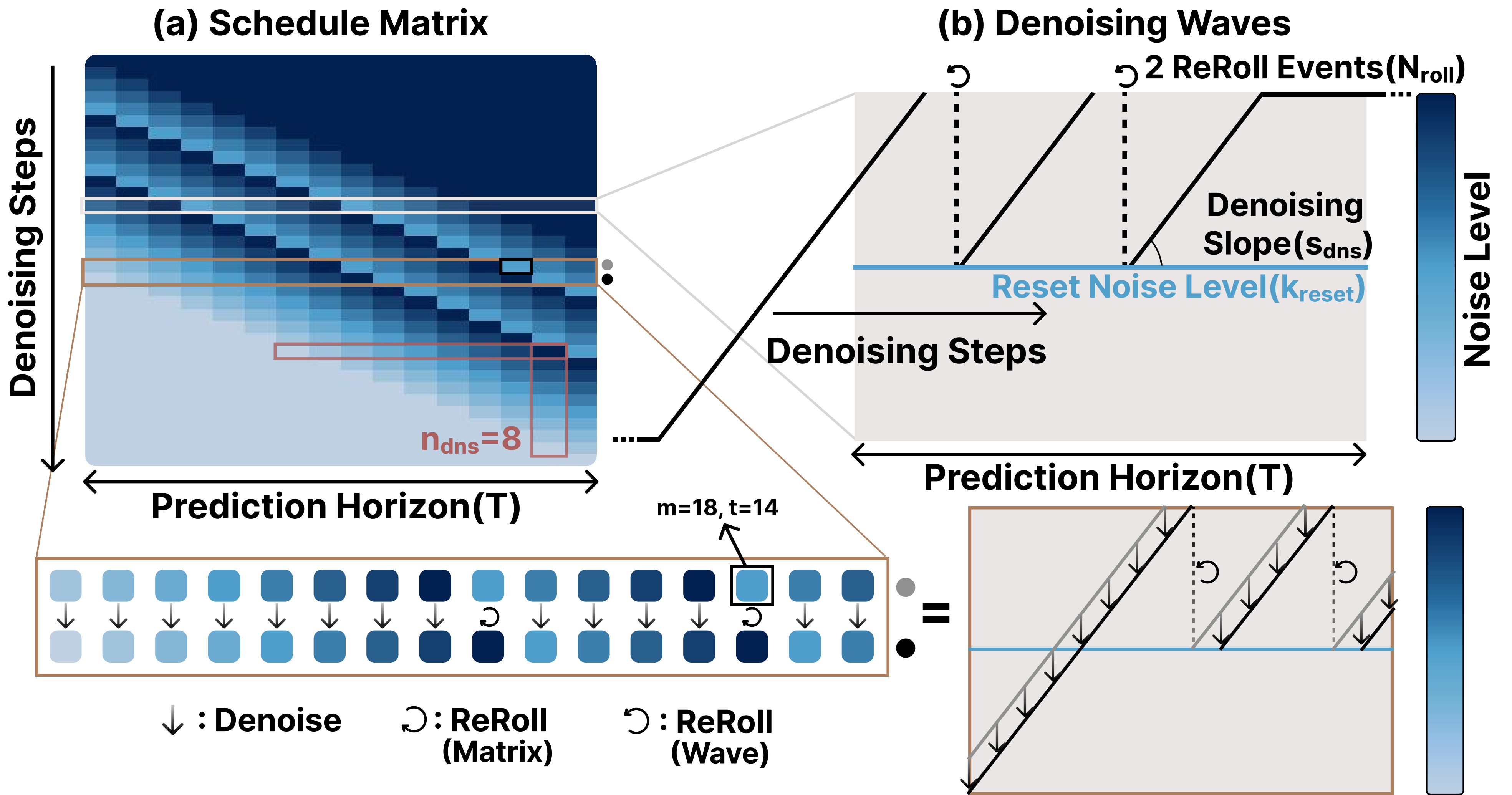
Consecutive schedule rows specify a DDIM denoising update, no change, or forward re-noising. Slope, reset threshold and reset-wave count control the pattern. Matrix and wave views depict the same process, rather than separate algorithms.
Denoising slope.
The denoising slope is horizon T divided by the updates required for one uninterrupted full-noise-to-clean wave. Larger slopes yield shorter chunks and more local refinement; smaller slopes span broader temporal context. The same slope can imply different numbers of updates at different horizons.
Reset noise level.
A chunk edge crossing the reset level triggers a return to K. Resetting too early discards useful refinement; resetting near zero makes the region almost deterministic before revision. Intermediate thresholds near the middle work well in the reported tests, without a universal optimality guarantee.
Number of ReRoll events.
N_roll counts restart waves, equivalently the maximum resets experienced by any token; it does not imply that all tokens reset equally often. Extra waves increase revision opportunity and sampling cost, with diminishing empirical returns.
Bidirectional schedule matrix.
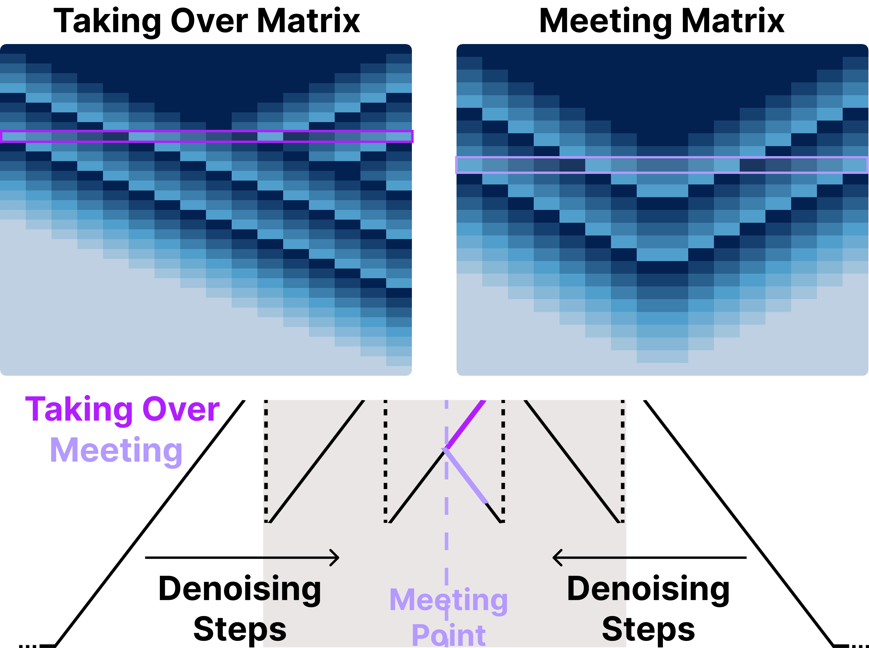
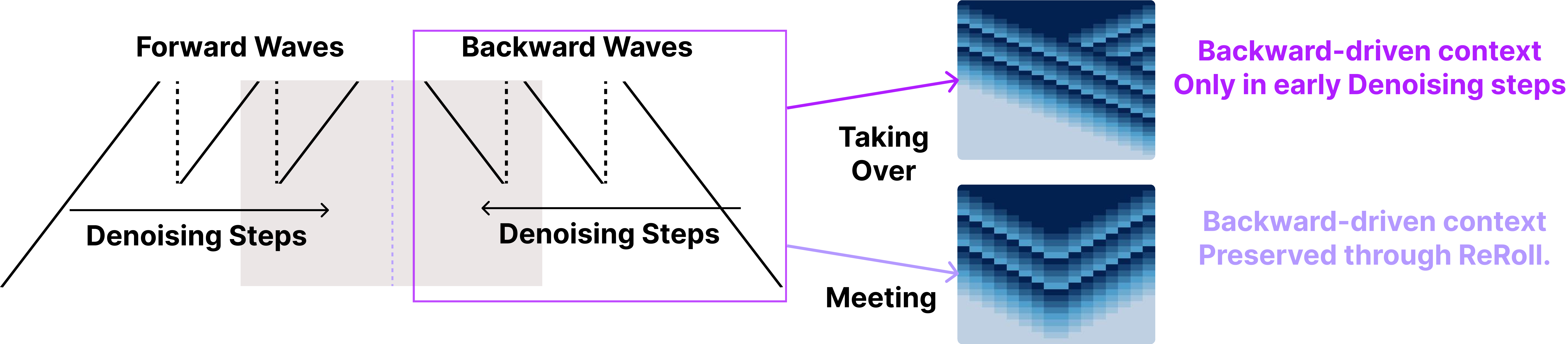
Bidirectional waves bring initial and terminal information toward an adjustable meeting point. The taking-over variant lets the forward wave dominate after overlap; the meeting variant preserves waves from both ends. Each direction may have different slope, threshold and event count. These schedules require noncausal attention to use information across the horizon.
3.2 Training with Linear Chunks
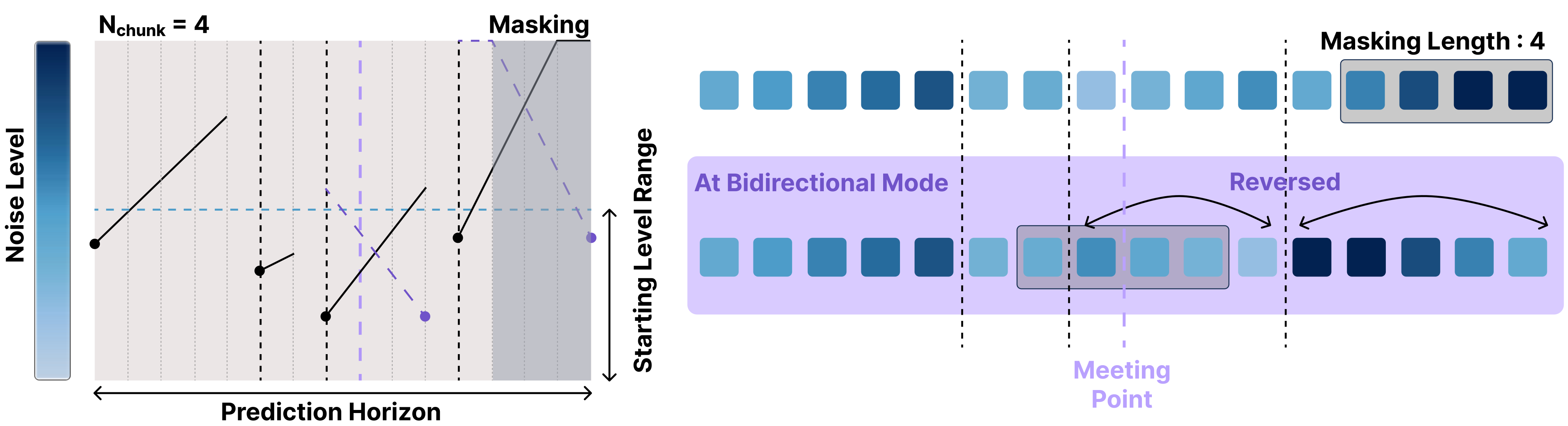
Training samples randomized chunk counts, boundaries, slopes and starting levels, covering more configurations than one deployment schedule while retaining local linear structure. Forward mode can mask a future suffix; bidirectional mode reverses right-side chunks and masks around the meeting region. The denoising objective remains standard regression. This structured training distribution is essential: applying ReRoll sampling alone to a Diffusion Forcing model gives inconsistent gains.
4 Experiments
Experiments compare full-sequence diffusion, Diffusion Forcing and ReRoll in four domains. DF and DR generally share backbone and representation; some full-sequence baselines differ in architecture, loss or masking. Main simulation results aggregate three training seeds after checkpoint selection; appendix single-seed maxima use a different reporting convention.
4.1 Effect of ReRoll and Training Alignment
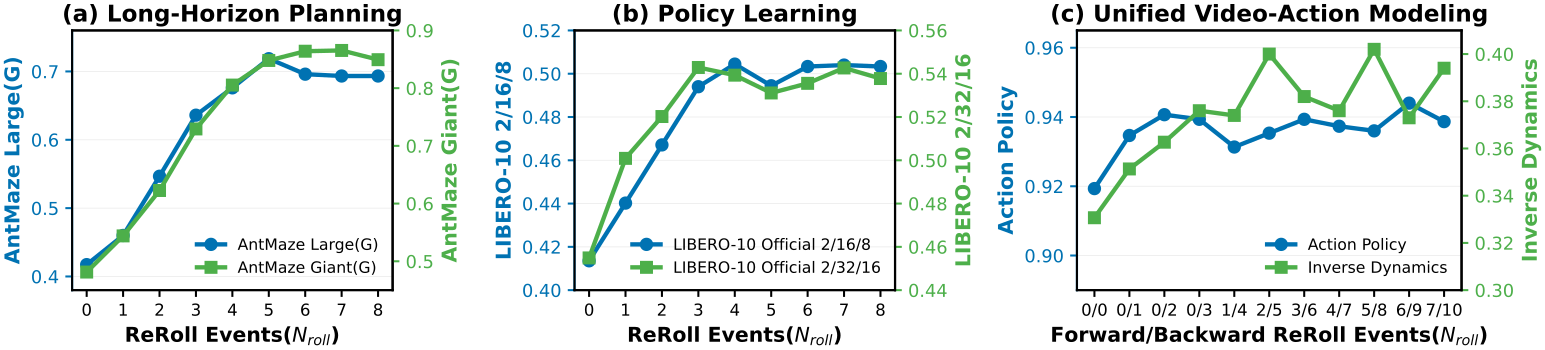
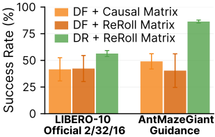
More ReRoll events improve success initially and then saturate. Random linear-chunk training makes the reset schedule effective; independently sampled token levels do not reliably support the same revisions. Both components matter in the ablation. Their contribution is empirical rather than a convergence theorem.
4.2 Long-Horizon Planning
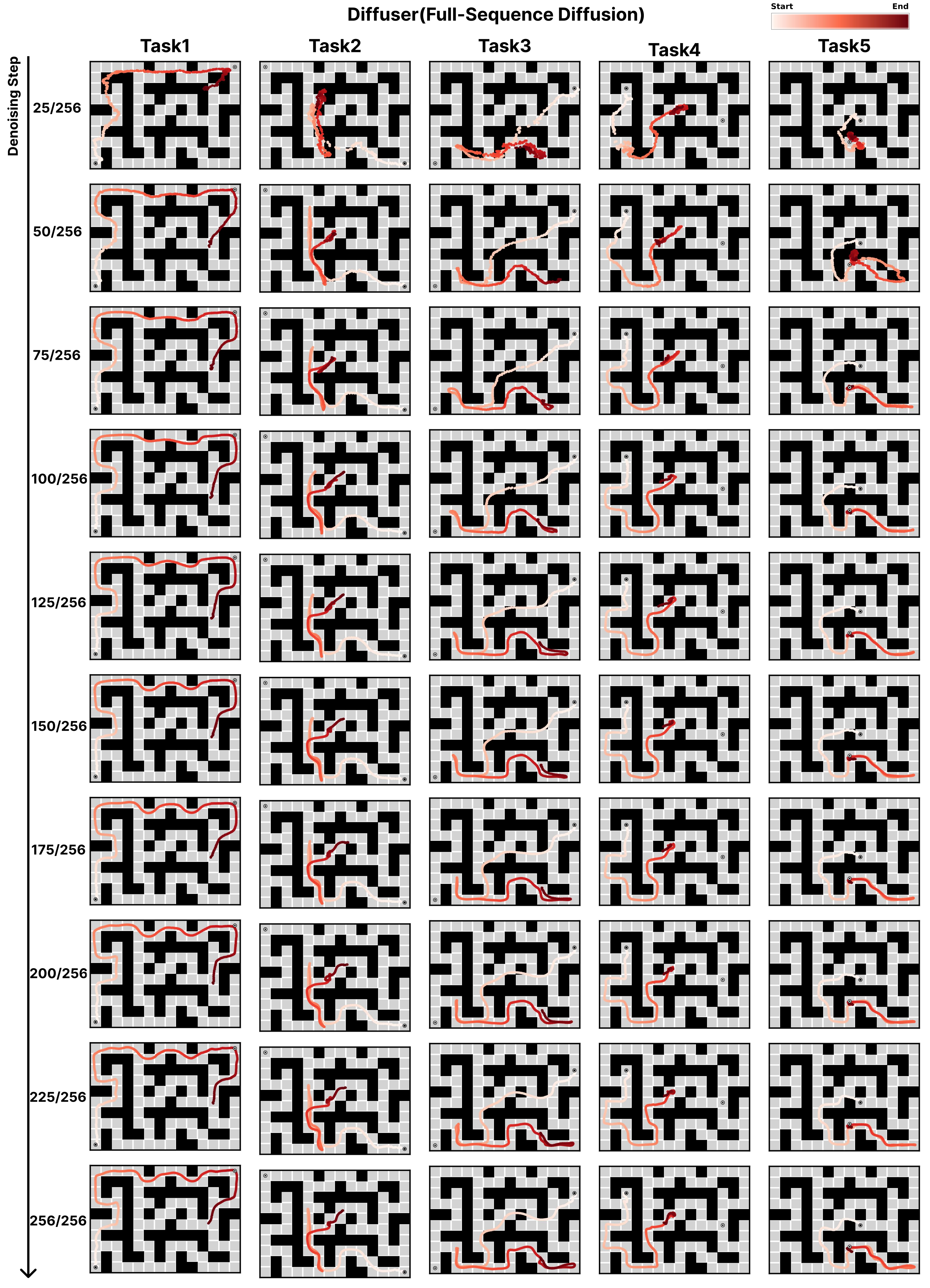
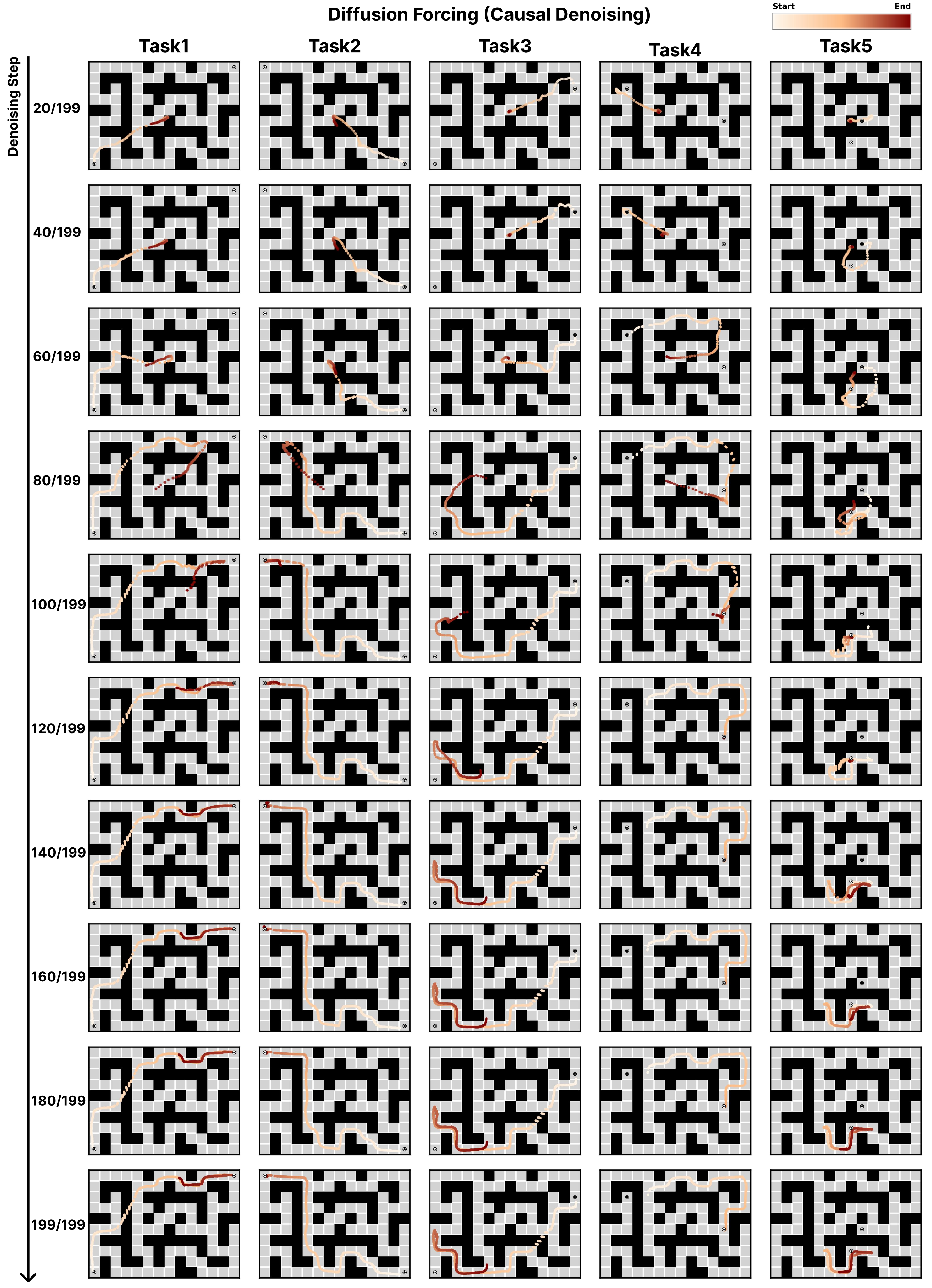
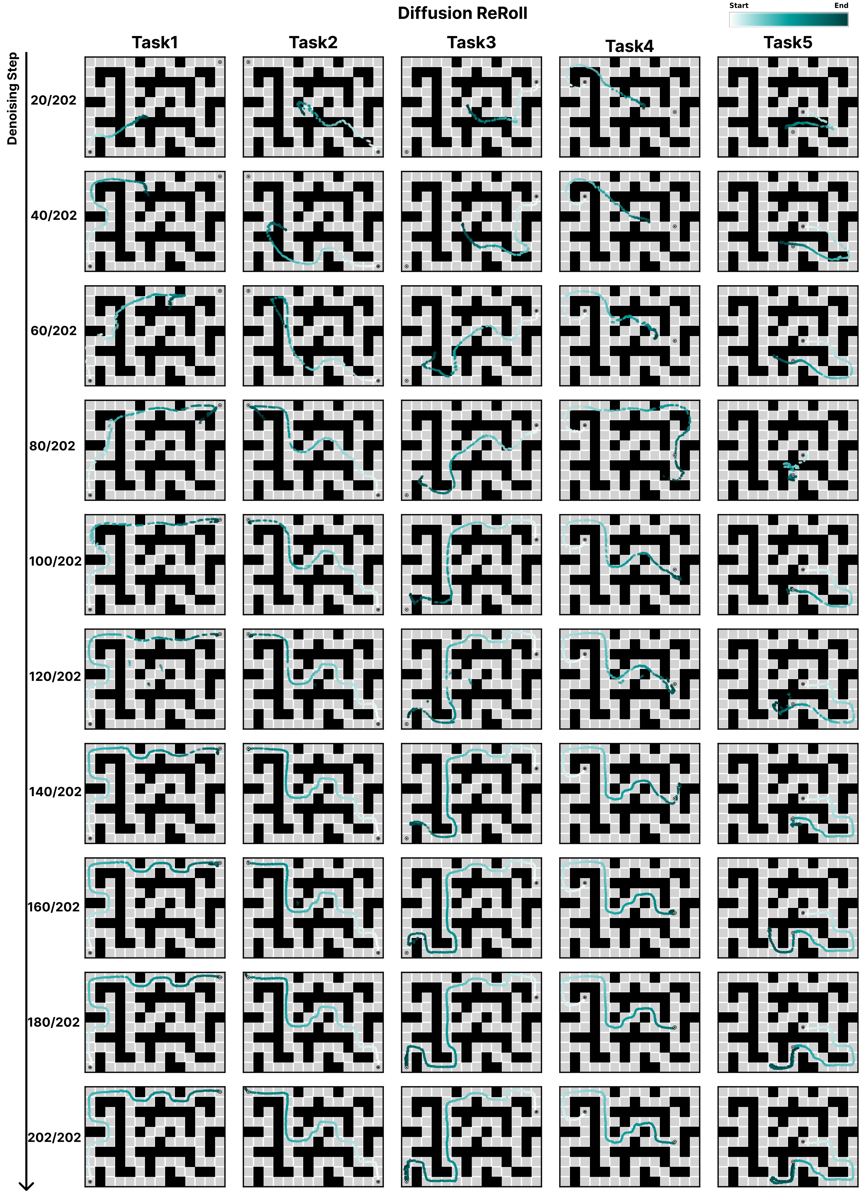
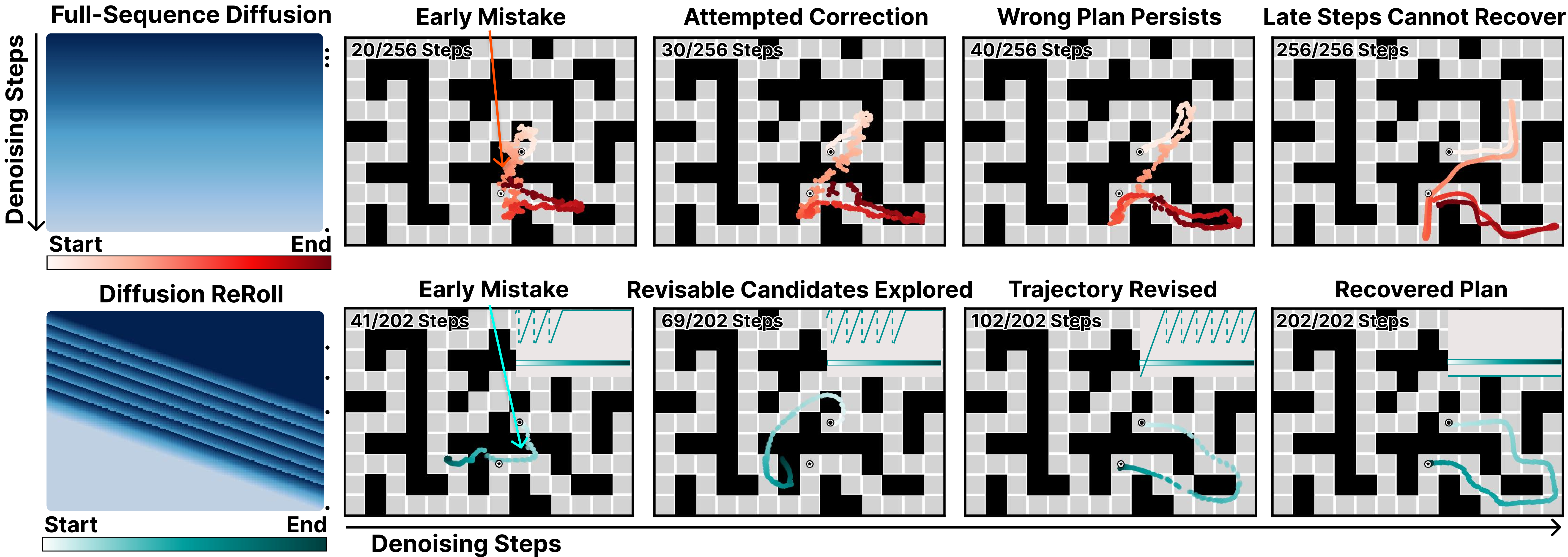
On six OGBench maze variants, ReRoll leads the reported guidance/replanning and goal-inpainting comparisons. Mean gains are 15.29 percentage points over DF in guidance, or about 21% relative, and 16.98 points over Diffuser in inpainting, or about 23% relative. Qualitative denoising sequences show recovery from wrong routes. The protocols use different goal handling and separately trained models; Diffuser uses a U-Net while DF/DR use Transformers.
| Mode | Method | AntMaze | PointMaze | ||||
| Giant | Large | Medium | Giant | Large | Medium | ||
| Guidance Replan | Diffuser | 16.0 1.1 | 42.1 4.2 | 69.1 1.0 | 26.5 4.9 | 30.0 1.8 | 46.4 0.8 |
| Forcing | 49.1 9.1 | 55.3 5.7 | 93.9 2.4 | 88.9 4.0 | 60.8 1.7 | 88.7 7.6 | |
| ReRoll | 86.4 1.4 | 69.6 1.4 | 98.0 0.4 | 99.3 0.8 | 76.3 1.8 | 98.8 0.4 | |
| Inpainting | Diffuser | 33.2 1.4 | 68.1 4.3 | 88.3 1.6 | 64.9 1.6 | 96.1 0.5 | 92.0 3.9 |
| Forcing | 71.9 4.0 | 67.5 0.6 | 90.5 0.6 | 94.5 1.6 | 95.7 1.8 | 91.2 2.8 | |
| ReRoll | 80.9 3.6 | 74.4 0.4 | 93.7 0.6 | 99.1 0.2 | 99.5 0.6 | 96.9 2.7 | |
4.3 Policy Learning
LIBERO-10 tests multi-task manipulation from scratch with scalar task identifiers, and RoboCasa tests four single-task settings. DF/DR predict anchor-relative cumulative actions, while the standard DP comparison also differs in representation and training details. ReRoll improves LIBERO averages under both reset protocols, but RoboCasa gains are less consistent. Opening the gripper at reset is materially easier and closer to demonstrations; official and open-reset scores must remain separate.
| Method | LIBERO-10 Official (Obs./Hor./Act.) | LIBERO-10 Open (Obs./Hor./Act.) | ||||||||
| 2/16/8 | 2/32/16 | 2/64/16 | 4/32/16 | 8/32/16 | 2/16/8 | 2/32/16 | 2/64/16 | 4/32/16 | 8/32/16 | |
| Diff. Policy | 28.1 3.8 | 41.1 8.2 | 35.1 2.7 | 42.2 8.8 | 53.8 0.9 | 76.2 0.5 | 65.5 1.9 | 57.9 2.0 | 69.1 1.4 | 64.7 1.9 |
| Forcing | 37.3 12.0 | 41.6 10.9 | 41.5 4.1 | 63.0 2.7 | 62.2 4.0 | 68.3 1.7 | 60.1 1.1 | 59.0 2.9 | 70.7 0.8 | 75.1 2.4 |
| ReRoll | 51.0 24.1 | 56.4 2.8 | 63.4 6.4 | 74.5 2.6 | 68.1 7.7 | 82.5 3.6 | 75.6 3.1 | 70.7 1.0 | 81.5 2.9 | 82.9 0.8 |
| Method | CloseSingleDoor | CoffeePressButton | CoffeeServeMug | PnPCounterToSink (300 Demos) | ||||||||
| 2/32/16 | 2/64/16 | 4/32/16 | 2/32/16 | 2/64/16 | 4/32/16 | 2/32/16 | 2/64/16 | 4/32/16 | 2/32/16 | 2/64/16 | 4/32/16 | |
| Diff. Policy | 52.0 2.0 | 52.7 2.3 | 56.7 8.3 | 76.0 5.3 | 54.7 8.3 | 80.0 4.0 | 43.3 3.1 | 32.7 4.2 | 39.3 5.8 | 30.7 3.1 | 22.0 4.0 | 24.7 2.3 |
| Forcing | 58.7 8.1 | 68.0 3.5 | 65.3 4.6 | 79.3 8.1 | 70.7 1.2 | 88.7 5.0 | 34.0 7.2 | 41.3 4.2 | 36.0 5.3 | 28.7 5.0 | 29.3 1.2 | 31.3 6.1 |
| ReRoll | 67.3 5.8 | 62.0 5.3 | 65.3 6.4 | 84.0 5.3 | 80.7 7.0 | 86.0 4.0 | 40.0 5.3 | 34.7 4.6 | 36.0 3.5 | 28.7 3.1 | 29.3 6.1 | 29.3 2.3 |
Reducing inference latency.
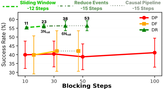
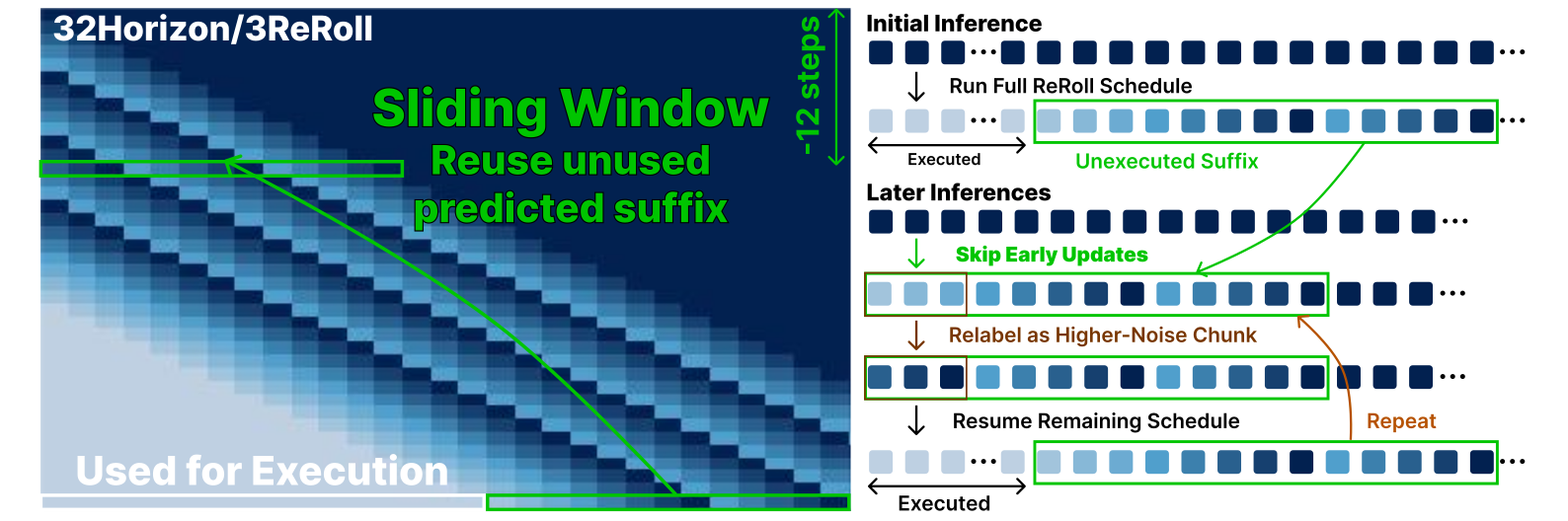
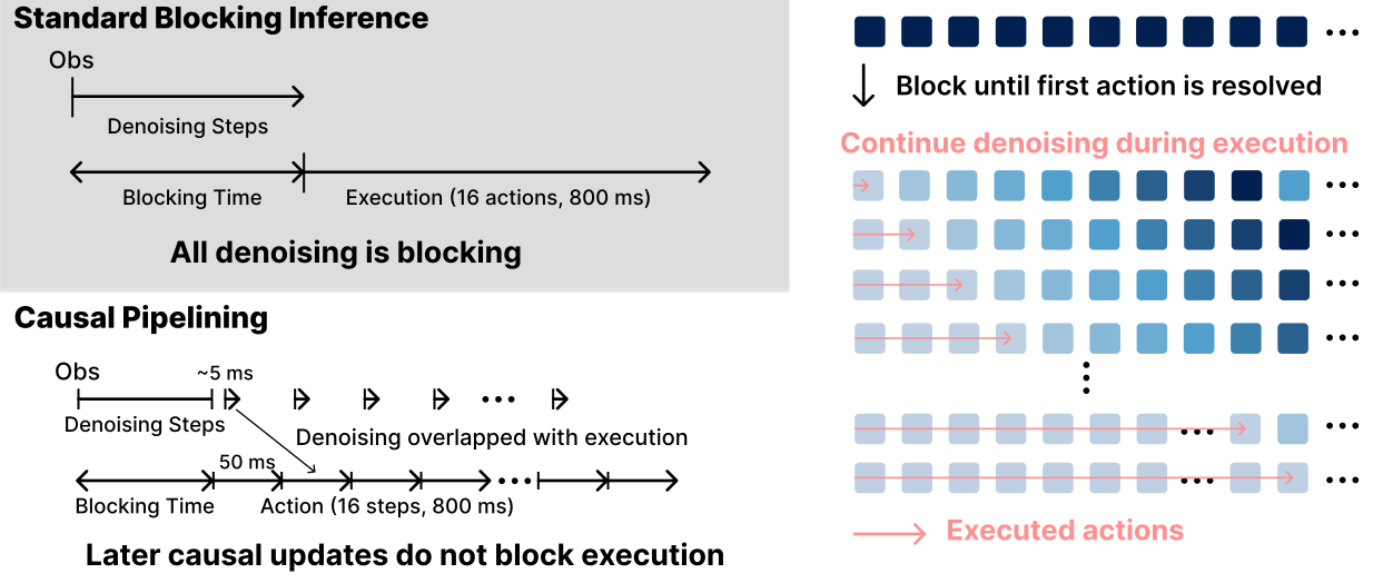
Fewer reset waves, reuse of an unexecuted action suffix and pipelining the final causal updates reduce blocking latency. The illustrated LIBERO schedule falls from 53 to 11 blocking updates while retaining high success. Pipelining overlaps computation with execution, so fewer blocking updates do not necessarily mean less total computation.
4.4 Unified Video-Action Modeling
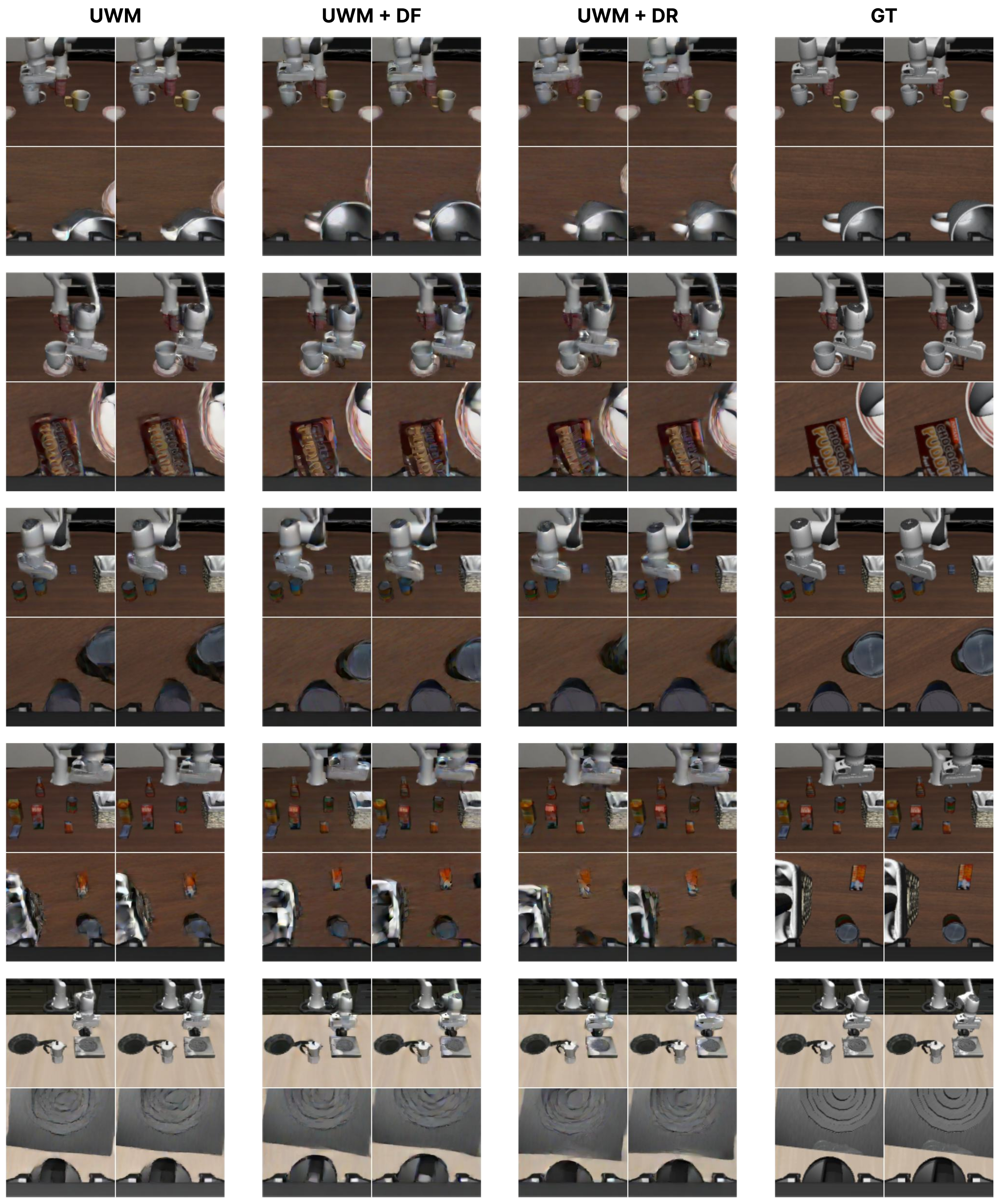
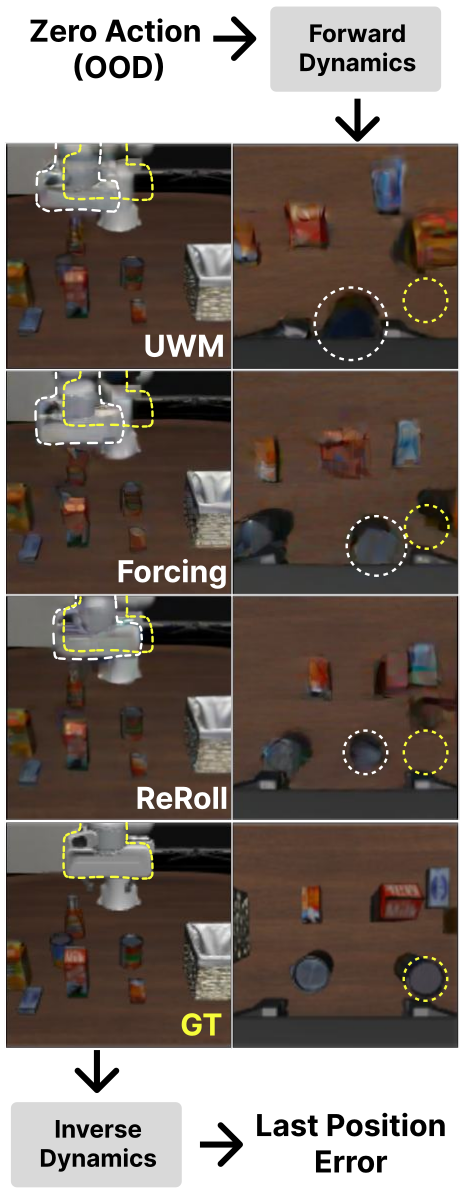
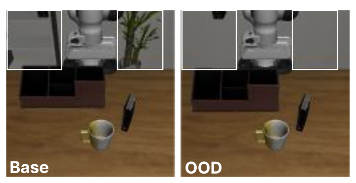
Within Unified World Models, schedules span 32 actions and two future video frames. DR improves action-only/joint policy success, inverse dynamics and robustness to enlarged object-position ranges and removed background objects: OOD joint-policy success is 69.7%, versus 58.1% for UWM and 60.7% for DF. A zero-action diagnostic also gives the lowest terminal displacement, about 0.301 m; this is still a substantial residual, not proof of physical consistency. The models share changes needed for token-level conditioning, and the appendix details important baseline/interface differences.
| Method | Act. Pol. (%) | Joint Pol. (%) | Inv. Dyn. (%) | OOD Act. (%) | OOD Joint (%) | Zero-Act. Err. (m) |
| UWM | 86.5 1.9 | 86.7 1.2 | 26.7 3.6 | 56.6 3.3 | 58.1 0.8 | 0.328 0.004 |
| UWM + DF | 90.8 0.7 | 90.6 3.7 | 32.0 1.3 | 61.1 2.2 | 60.7 2.7 | 0.317 0.012 |
| UWM + DR | 94.4 0.9 | 93.9 0.8 | 37.3 0.8 | 67.9 2.8 | 69.7 2.0 | 0.301 0.003 |
4.5 Real-World Navigation
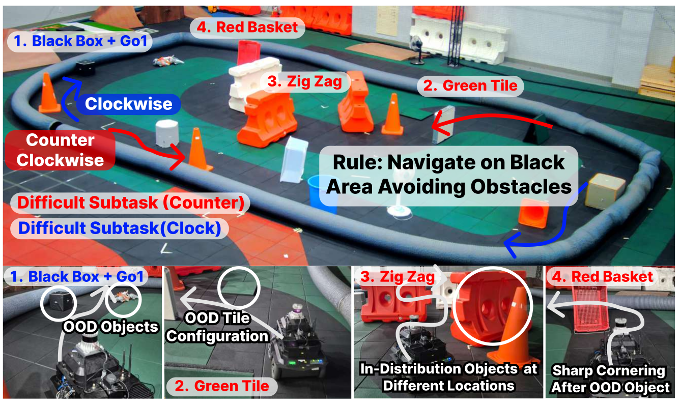
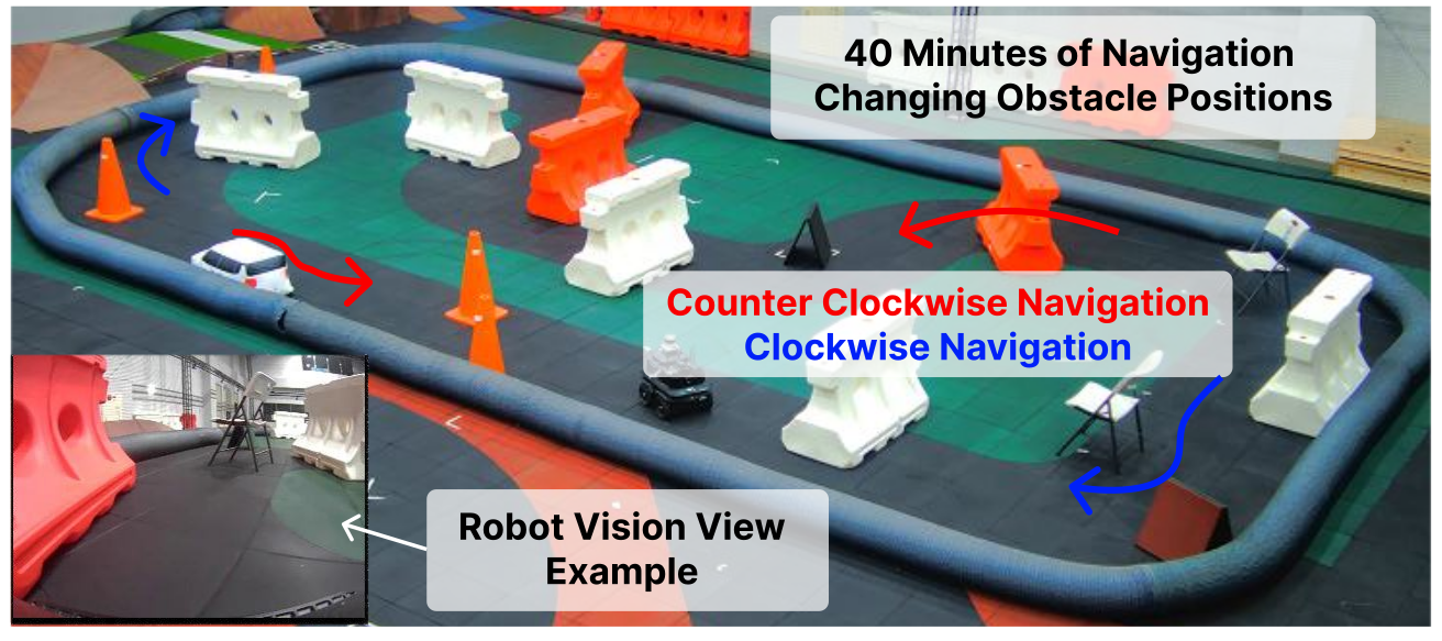
A Jackal robot follows a marked course from a single RGB image using approximately 40 minutes of demonstrations. Sixteen predicted waypoints span 3.2 seconds; an inverse model maps the first eight to one velocity command at each 5 Hz update. DR has the highest mean under tested obstacle, floor and lighting shifts, with onboard RTX 3060 inference. Trials cover repeated directions/subtasks within one course, not many independent environments.

5 Limitations
New tasks may require tuning both training noise profiles and deployment schedules to balance performance and inference cost. Evidence for cross-horizon revision is empirical: the paper gives neither a theoretical characterization of when it helps nor convergence guarantees. Tests use Transformer denoisers and benchmark-scale datasets; large general-purpose robot models remain unvalidated.
6 Conclusion
Structured re-noising and aligned training make sequence predictions revisable across time. The evidence supports this mechanism in the tested planning, manipulation, video-action and navigation settings, while leaving schedule design and wider generalization unresolved.
Acknowledgments
The work was funded through a 2026 Korean Government Agency for Defense Development grant. The authors acknowledge help with navigation deployment, manuscript feedback and peer review.
Appendix
The appendices specify schedule transitions, training distributions, action representations, evaluation protocols, latency and additional quantitative/qualitative results.
Appendix A Choosing the Schedule Matrix
Schedule design controls both information flow and compute. The appendix distinguishes DDIM denoising from stochastic upward noise transitions and describes forward/bidirectional schedules, parameter ablations and deployment optimizations.
A.1 Schedule-Matrix Sampling and DDIM Updates
Map discrete schedule levels to training diffusion times, with clean level mapped to time −1 and unit cumulative alpha. Downward transitions use DDIM with eta zero; upward transitions apply the forward Gaussian corruption kernel; equal levels leave tokens unchanged. Thus deterministic DDIM does not make the full ReRoll process deterministic: every reset injects fresh noise. All transition formulas and endpoints are retained.
Equations 3–6
| (3) |
| (4) |
| (5) |
| (6) |
A.2 Bidirectional Schedule Matrices
A bidirectional schedule assigns forward/backward waves to regions around a meeting point. Taking-over uses backward context initially and then forward refinement; meeting keeps both directions active. Directional slopes and reset counts can differ, allowing endpoint conditions to influence the unresolved interior.

A.2.1 Applications to Maze Planning
Maze goal inpainting benefits from bidirectional context; the displayed taking-over schedule is the primary choice. Additional guidance results in Table 5 explore bidirectionality using one seed, whereas the forward comparison summarizes three seeds. This exploratory comparison should not be read as a fully replicated superiority claim.
| Task | Forward matrix | Bidirectional taking over |
| AntMaze Giant | 86.4 1.4 | 87.2 |
| AntMaze Large | 69.6 1.4 | 77.6 |
| AntMaze Medium | 98.0 0.4 | 97.6 |
| PointMaze Giant | 99.3 0.8 | 100.0 |
| PointMaze Large | 76.3 1.8 | 74.4 |
| PointMaze Medium | 98.8 0.4 | 100.0 |
A.2.2 Applications to Unified Video-Action Modeling
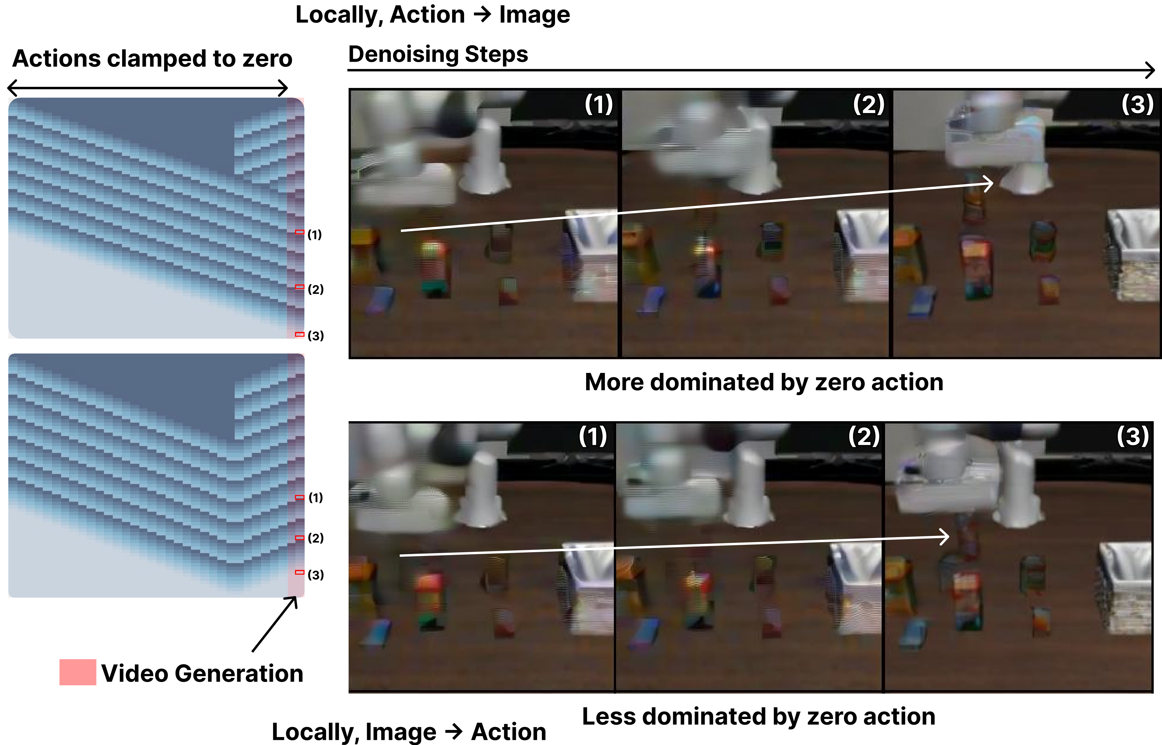
Joint video/action modeling uses the meeting schedule to balance early actions and terminal frames; taking-over can let forward zero-action context dominate generated images. The qualitative zero-action experiment clamps action values but continues their schedule noise labels, unlike the quantitative zero-inpainting diagnostic. Meeting and taking-over results therefore probe information flow, not an identical physical-consistency test.
A.3 ReRoll Schedule Ablations
The ablations vary horizon, reset threshold and slope. Their settings and checkpoint aggregation differ in places from the main tables, so numerical values are not all directly interchangeable.
A.3.1 Same ReRoll Parameters at Different Horizons
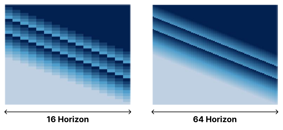
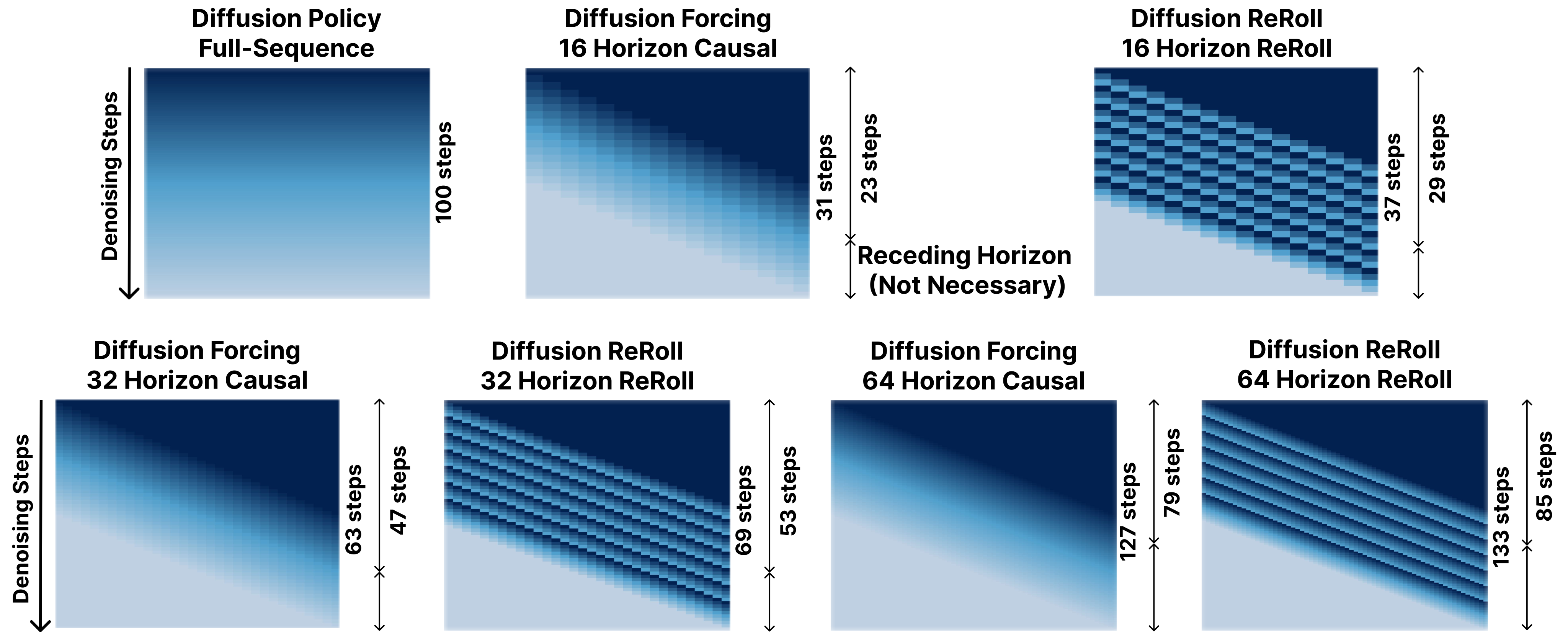
Keeping slope, reset threshold and event count fixed while increasing horizon preserves the wave pattern but increases chunk extent and sampling rows. The side-by-side matrices show that identical parameter values do not imply equal compute or identical token-wise context.
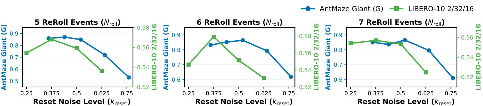
A.3.2 Effect of Reset Noise Level
Middle reset levels generally outperform very early or late resets. For short horizons, discretization restricts thresholds to a few distinct effective levels. LIBERO averages the best checkpoint with its two neighbors before averaging three seeds, whereas the maze experiment uses each seed’s best checkpoint. Error bars reflect this stated procedure.
A.3.3 Results with Lower Denoising Slopes
Lower slopes can also work when the training chunk distribution is adjusted accordingly. Table 6 presents example configurations, not a controlled single-variable comparison establishing a universally better slope. Training and deployment schedules must be interpreted together.
| Task | Schedule matrix | Training chunks | Setting | Success rate | |||||
| Slope range | Start range | Main / Official | Open | ||||||
| Default schedule used in main experiments | |||||||||
| AntMaze Large | 4 | 0.52 | 6 | 8 | Guidance | 69.6 1.4 | – | ||
| AntMaze Giant | 4 | 0.52 | 6 | 8 | Guidance | 86.4 1.4 | – | ||
| LIBERO-10 | 4 | 0.50 | 6 | 8 | 2/16/8 | 51.0 24.1 | 82.5 3.6 | ||
| Lower-slope example configurations | |||||||||
| AntMaze Large | 1 | 0.52 | 2 | 4 | Guidance | 66.4 | – | ||
| AntMaze Large | 2 | 0.52 | 3 | 6 | Guidance | 69.2 | – | ||
| AntMaze Giant | 2 | 0.52 | 3 | 6 | Guidance | 74.0 | – | ||
| LIBERO-10 | 2 | 0.50 | 2 | 4 | 2/16/8 | 47.2 13.2 | 77.0 2.8 | ||
A.4 Sampler Update Counts and Inference Time
Sampler updates equal traversed schedule rows minus one, not simply the number of ReRoll events. Policy sampling can stop once the executable prefix is clean. At six waves, reported counts are 202 for maze planning; 29, 53 and 85 for policy horizons 16, 32 and 64; and 70 for video-action generation. Longer horizons and extra resets increase cost.
| Planning | Policy learning | Unified Video-Action | |||
| 16/8 | 32/16 | 64/16 | |||
| 0 | 124 | 11 | 23 | 31 | 34 |
| 1 | 137 | 14 | 28 | 40 | 40 |
| 2 | 150 | 17 | 33 | 49 | 46 |
| 3 | 163 | 20 | 38 | 58 | 52 |
| 4 | 176 | 23 | 43 | 67 | 58 |
| 5 | 189 | 26 | 48 | 76 | 64 |
| 6 | 202 | 29 | 53 | 85 | 70 |
| 7 | 215 | 32 | 58 | 94 | 76 |
| 8 | 228 | 35 | 63 | 103 | 82 |
Policy inference time.
On one RTX A5000 with batch size one, timings average 30 runs after ten warm-ups and include image encoding/action generation but exclude environment stepping, media writing and action unnormalization. Three-wave DR takes about 83/156/230 ms at horizons 16/32/64; six-wave DR about 123/225/346 ms. DP uses 10/30/50 DDIM updates or a 100-step DDPM comparison. These are full-inference measurements, distinct from blocking latency after pipelining.
| Sampler | O2/H16/A8 | O2/H32/A16 | O2/H64/A16 |
| DP, 10 DDIM | 10 / 44.7 1.7 | 10 / 44.9 1.6 | 10 / 46.5 3.7 |
| DP, 30 DDIM | 30 / 121.6 4.9 | 30 / 123.6 2.7 | 30 / 121.1 4.4 |
| DP, 50 DDIM | 50 / 207.4 12.6 | 50 / 203.9 9.0 | 50 / 194.8 3.8 |
| DP, 100 DDPM | 100 / 390.7 7.7 | 100 / 421.1 34.6 | 100 / 387.4 10.9 |
| DR, 3 ReRoll | 20 / 82.8 5.4 | 38 / 155.9 7.3 | 58 / 229.8 5.6 |
| DR, 6 ReRoll | 29 / 123.1 2.4 | 53 / 225.2 4.7 | 85 / 346.3 4.6 |
A.5 Inference Time Optimization
Deployment reuses previous predictions and overlaps denoising with execution. The objective is to reduce updates blocking the next action chunk; changes in responsiveness and total compute are distinct.
Sliding-window reuse.
Shift the unused suffix to the next prediction window, decode it into physical per-step actions and re-encode cumulative actions with the new horizon indices. If the new schedule requests a higher noise level, the implementation relabels the reused values without adding Gaussian noise. This is an explicit inference heuristic, not the forward corruption transition. The first prediction uses the ordinary schedule.
Causal pipelining.
Once early actions are usable, execute them while completing updates for later actions. A 50 ms control step permits overlapping several roughly 5 ms denoising updates in the illustrated setup. Causal structure permits overlap, but observation/action timing still affects the effective closed-loop policy.
Latency reduction.
For the 2/32/16 LIBERO example, blocking updates fall 53→38 with pipelining, then to 23 with three rather than six ReRoll waves, then to 11 with suffix reuse. A longer 64-step example falls 85→70→34 using pipelining/reuse. These reductions depend on the chosen execution horizon and schedule; they are not universal speedup factors.
Appendix B Training Details for Diffusion ReRoll
Training randomizes piecewise-linear noise profiles, retains full attention, reweights denoising loss and adapts action representation/backbone interfaces. All original mathematical definitions and hyperparameter tables remain available.
B.1 Noise Distribution for Training
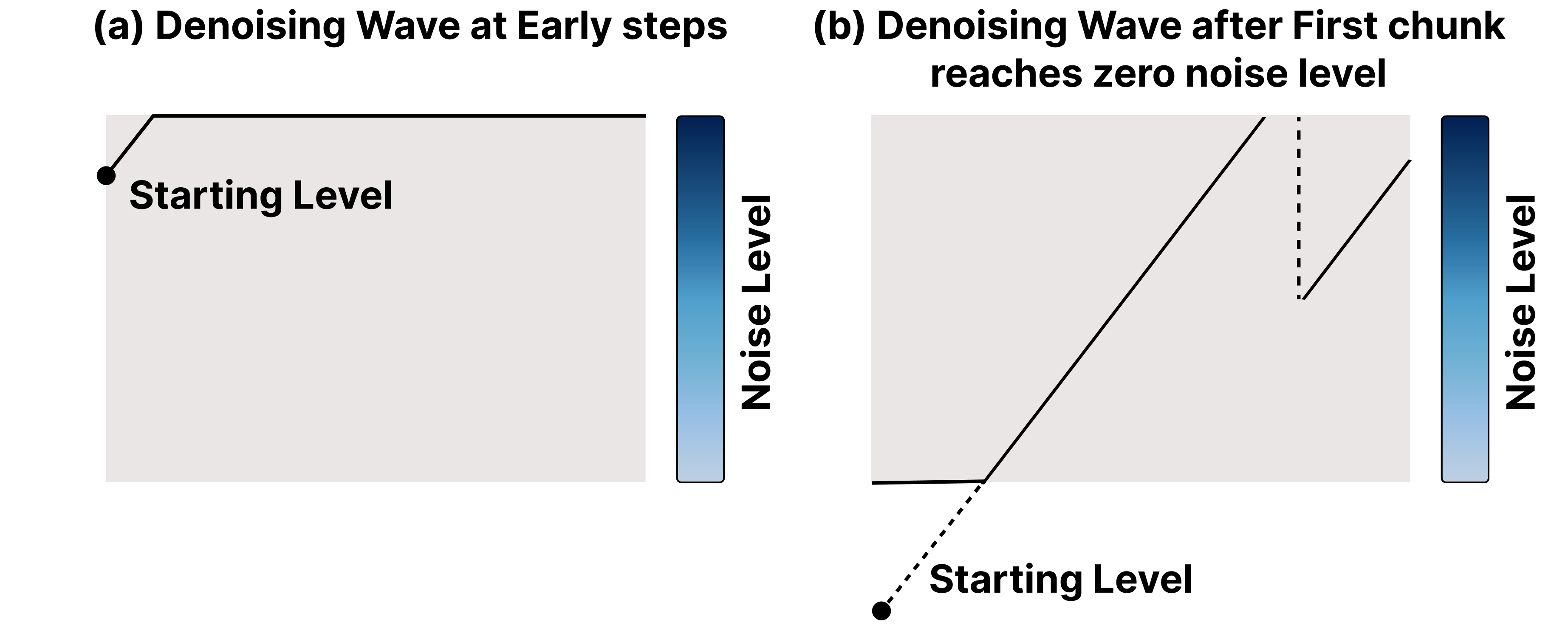
Sample chunk boundaries and local slopes, assign starting levels and clip the resulting profile into the legal noise range. A random masked suffix or bidirectional central region broadens missing-context configurations. The distribution intentionally covers, but does not exactly replay, deployed schedules.
B.1.1 First-Chunk Noise Assignment
The first chunk samples a wider offset range, including values that clip to a clean prefix and values near full noise. This exposes the model to varied history visibility and start conditions, rather than fixing the first token at one noise level.
Equations 7–8
| (7) |
| (8) |
B.1.2 Bidirectional Mode Noise Assignment
Training mixes forward, masked-bidirectional and full-horizon-bidirectional branches. The latter removes the central mask while still reversing selected right-side chunks; the entire trajectory is never reversed. Optional near-clean inpainting uses levels up to 0.25K, conditioned on either bidirectional branch. For example, a combined bidirectional probability of 0.5 and conditional inpainting probability of 0.1 yields 5% overall. DF controls use matched masking without linear chunks.
Equations 9–10
| (9) |
| (10) |
B.1.3 Chunk Slope Range
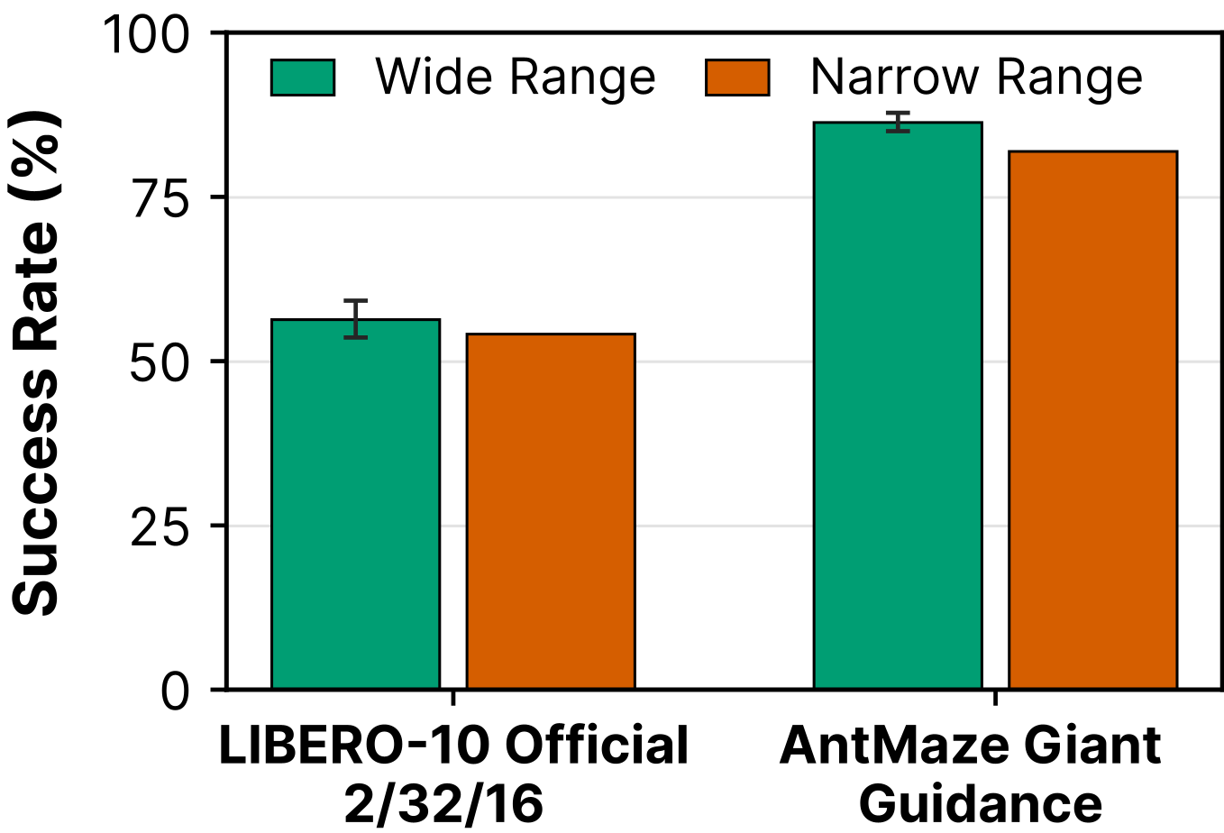
Chunk slopes span 0.5–2.5 times the deployment slope in the main setup. A narrower 0.875–1.125 range performs somewhat worse in the displayed LIBERO ablation, supporting diverse structured profiles over narrowly copying the deployment wave.
Equations 11–12
| (11) |
| (12) |
B.1.4 Starting-Level Range
Later chunks start within a low-to-middle noise interval, whereas the first has a broader range. This choice covers varied local stages of the denoising/re-noising cycle. The exact sampling bounds and clipping formulas are retained.
Equation 13
| (13) |
B.2 Important Components for Diffusion ReRoll Training
The authors retain much of the baseline optimization recipe, while attention direction and loss weighting are central to the method. Reusing those settings does not eliminate the need to choose schedule and representation parameters.
B.2.1 Low Sensitivity to Basic Learning Parameters
The implementation largely retains learning rates, optimizers, batches and training durations from baseline codebases rather than introducing a separate optimization recipe. The authors recommend tuning schedule/noise-distribution parameters first on new tasks. This reuse supports practical compatibility; the section does not present an exhaustive learning-hyperparameter sensitivity sweep.
B.2.2 Necessity of Non-causal Training
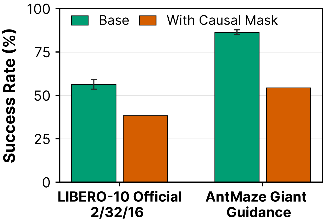
Causal attention substantially degrades DR on both LIBERO-10 and AntMaze Giant in Figure 23. Noncausal attention lets resolved future context influence earlier tokens and supports the intended cross-horizon revision mechanism. This figure is a DR masking ablation, not a separate test of both DR and DF.
B.2.3 SNR Reweighting
DF/DR regress clean samples with min-SNR weighting, clipping at 2.5 for action-style outputs and 5 for images. This limits domination by particular noise levels. Standard DP uses noise prediction and uniform weighting, so the DP comparison does not vary the schedule alone. Min-SNR weighting supplies the underlying reweighting method.
Equations 14–16
| (14) |
| (15) |
| (16) |
B.3 Action Representation for Manipulation
Manipulation actions become anchor-relative cumulative positions and rotations, while the gripper stays noncumulative. Cumulative targets are explicitly predicted so revising an early token need not mechanically shift every later target. Positions sum normalized deltas; rotations compose before normalization. This distinction matters when reconstructing metric executable actions.
Equation 17
| (17) |
Horizon-dependent scaling.
Fit horizon-dependent power-law scales to training-set variation and normalize cumulative position/rotation targets by their index-dependent scale. Position and rotation use different prefactors. The exact formulas remain visible because normalization changes both training magnitude and suffix-reuse conversion.
Equation 18
| (18) |
Conversion to executable actions.
Invert the horizon scaling, then recover per-step translation differences and relative rotations between consecutive cumulative predictions. Convert back to physical action coordinates for execution. Reuse must decode and re-encode at the shifted horizon indices rather than copying normalized cumulative values directly.
Equation 19
| (19) |
Diffusion Policy with the same representation.
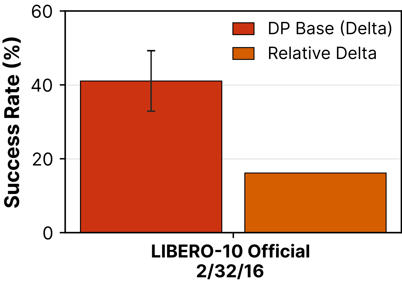
Giving DP the same cumulative representation worsens its displayed result, so representation alone does not explain DR’s gain. Nevertheless DP and DF/DR also differ in masking, objective and noise conditioning, preventing a pure one-factor attribution from this comparison.
B.4 Model Architecture
The method reuses established backbones with token-level noise conditioning. Dataset-specific architectural changes and pretraining choices are detailed below and in the original tables.
Long-horizon planning.
DF/DR use full-attention Transformer denoisers for maze planning. Diffuser uses its U-Net: a tested full-sequence Transformer performed poorly, including 4% AntMaze Giant and 34.4% Large guidance success. This pragmatic baseline choice introduces an architecture difference into planning comparisons.
Policy Learning.
DF/DR modify the Chi-Transformer with per-token noise embeddings, full attention and sinusoidal action positions, adding roughly 1.1% parameters. DP retains its standard causal mask/noise-prediction setup. Image observations share an encoder across methods within each experiment.
Equation 20
| (20) |
Unified Video-Action Modeling.
UWM originally conditions modalities through separate diffusion times in adaptive normalization. DF/DR instead concatenate per-token time embeddings, remove that time signal from AdaLN, use continuous action/image positions with sinusoidal embeddings and change temporal patch stride from two to one. These adaptations enable frame-specific schedules but also qualify architectural equivalence to the original UWM.
Real-World Navigation.
Navigation uses a modified Chi-Transformer with a jointly fine-tuned pretrained ResNet-50 and sinusoidal waypoint positions. A separate inverse-dynamics MLP converts the first eight waypoints into one linear/angular velocity command.
Appendix C Experiment Settings
Experimental details define the actual comparison: datasets, goal handling, reset protocols, seed/checkpoint selection, prediction/execution horizons and timing. These choices explain several apparent discrepancies among result tables.
C.1 Relative gain calculation
Relative gain divides the success-rate difference by the baseline rate. Maze guidance improves 72.78→88.07%: 15.29 percentage points, about 21% relative. Inpainting improves 73.78→90.76%: 16.98 points, about 23% relative. LIBERO’s official mean improves 40.06→62.70%: 22.64 points, about 56.5% relative. The source prose uses 40.06% for the LIBERO baseline while its displayed calculation rounds it to 40.07%; the original formula is preserved.
Equations
C.2 Long-Horizon Planning
PointMaze and AntMaze use OGBench offline trajectories, with medium/large/giant variants and separate guidance/replanning and goal-inpainting settings. The retained tables specify horizons, denoising schedules and training hyperparameters.
C.2.1 Evaluation Settings
Guidance and inpainting answer different planning questions and use separately trained models. A fixed low-level controller executes generated state trajectories, so overall success includes that controller’s tracking behavior.
Guidance-based replanning.
Guidance conditions on the goal through a sampling objective and replans every 50 environment steps. Prediction uses 100 tokens, stacking five states for medium/large mazes and ten for giant mazes. Episode limits are 1,000 or 1,500 steps. The guidance comparison uses matched goal-handling settings for DF and DR.
Equation 21
| (21) |
Goal inpainting.
Inpainting fixes goal conditions and generates one trajectory without replanning. After consuming it, the controller tracks the penultimate state rather than repeatedly commanding the inpainted goal; this avoids a trivial unlimited goal-tracking shortcut. DF receives a compatible bidirectional mask/schedule without resets.
Low-level execution.
PointMaze uses a heuristic position/velocity tracker, adding velocity information unavailable in the original OGBench state representation. AntMaze uses the learned low-level controller from Monte Carlo Tree Diffusion, targeting ten steps ahead and advancing when within distance 1.0. These controllers and thresholds are part of the evaluation, not learned by ReRoll.
Equation 22
| (22) |
C.2.2 ReRoll Parameters for Long-Horizon Planning
The displayed matrices use forward DR for guided replanning and a taking-over bidirectional schedule for goal inpainting. Main experiments use six ReRoll waves with task-family-specific parameters; schedule lengths are chosen near the baseline budget, not identically across all domains.

| Parameter | Value |
| Prediction horizon | 100 |
| Denoising slope | 4 |
| ReRoll events | 6 |
| Reset noise level | |
| Training chunk count | – |
| Chunk slope range | |
| Starting-level range | |
| Forward branch probability | 0.475 |
| Bidirectional branch probability | 0.475 |
| Full-horizon branch probability | 0.05 |
| Inpainting-mask probability | 0.1 |
C.2.3 Training and Sampling Hyperparameters
The original training/sampling table records dataset sizes, architecture, optimization, goal-conditioning and schedule settings. Main maze results average each training seed’s selected best checkpoint. Separately trained guidance/inpainting models and U-Net-versus-Transformer differences limit a purely sampler-only interpretation.
| Hyperparameter | Diffuser | DF / DR |
| Optimizer | AdamW | AdamW |
| Learning rate | ||
| Weight decay | ||
| Warmup steps | ||
| LR schedule after warmup | constant | constant |
| Batch size | 32 | 2048 |
| Max training steps | M | |
| Evaluated checkpoints | k–M, every k | k–k, every k |
| EMA | decay | not used |
| EMA start / update | / every steps | – |
| Training diffusion steps | 256 | 1000 |
| Noise clip | 20.0 | 20.0 |
| Beta schedule | cosine | linear |
| Prediction objective | prediction | prediction |
| Loss weighting | uniform elementwise MSE (no SNR weighting) | min-SNR, clip |
| Guidance scale | 0.1 | 2.0 |
| Training window | task horizon | 100 tokens |
| Backbone | Temporal U-Net | Transformer |
| Backbone size | channels , kernel 5 | width 128, 12 layers, 4 heads, FFN 512 |
C.3 Policy Learning
Manipulation evaluation covers LIBERO-10 multi-task learning and four RoboCasa single tasks. Observation history, prediction horizon and execution prefix are denoted Obs./Hor./Act.; scores average task success after per-seed checkpoint selection.
C.3.1 Evaluation Environment Settings
LIBERO is trained from scratch with task IDs, no language encoder and no policy pretraining. RoboCasa uses ImageNet-pretrained vision because from-scratch training did not converge in the tested setup. Methods within a task share observation/data handling.
Observations.
Observations combine camera images and robot state. LIBERO crops 128-pixel images to 76 pixels; RoboCasa uses 116-pixel crops and three cameras. RoboCasa predicts seven of the environment’s twelve action dimensions for the selected tasks. Such preprocessing choices remain fixed within each method comparison.
Encoders and data splits.
LIBERO uses 50 demonstrations per task with a 45/5 train/validation split varying across three seeds, yielding 450 training demonstrations per seed. RoboCasa has 50 demonstrations for three tasks; counter-to-sink uses 300, comprising 50 human and 250 MimicGen examples, with task-specific validation sets. Pretrained ResNet-18 is used for RoboCasa vision.
Checkpoint selection
Reported scores select checkpoints using evaluation rollouts: LIBERO evaluates up to 25 checkpoints from epochs 210–450 at intervals of ten, with 50 initial states per task. RoboCasa evaluates 31 or 15 checkpoints depending on data regime, also using 50 rollouts. Selecting the maximum on these rollouts can make reported success optimistic; it is not a clean held-out model-selection protocol. Three training seeds are then aggregated.
C.3.2 LIBERO-10 Reset Protocol
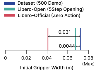
Demonstrations begin with gripper width about 0.07246 m; open reset is about 0.06811 m and official reset about 0.04135 m. The official state is therefore farther from the demonstrated initial condition. For DP at 2/16/8, opening raises success from 28.1% to 76.2%. Both protocols are retained; their results should not be pooled as equivalent conditions.
C.3.3 Applied ReRoll Parameters
Policy matrices stop when the executable prefix is resolved, leaving unnecessary suffix updates undone. With six ReRoll waves, horizons 16/32/64 use 29/53/85 deployed updates; the full matrices contain more rows. The retained figure distinguishes full schedule length from receding-horizon execution cost.
| Parameter | Value |
| Prediction horizon | |
| Denoising slope | 4 |
| ReRoll events | 6 |
| Reset noise level | |
| Training chunk count | – |
| Chunk slope range | |
| Starting-level range |
C.3.4 Basic Learning Hyperparameters
The detailed table preserves optimization, batch sizes, schedules, vision initialization, crop sizes and training durations. DF/DR use clean-target min-SNR loss and noncausal attention; DP uses noise-target uniform loss and its standard mask. These controlled and uncontrolled differences should be considered together.
| Hyperparameter | Diffusion Policy | DF / DR |
| Backbone | Chi-Transformer | Chi-Transformer |
| Action positional embedding | learnable | sinusoidal |
| Noise conditioning | global timestep token | per-token noise embedding |
| Causal attention mask | used | not used |
| Dropout | 0.1 | 0.01 |
| Optimizer | AdamW | AdamW |
| Policy learning rate | ||
| Visual encoder learning rate | ||
| Weight decay | 0 | 0 |
| Warmup steps | 200 | 200 |
| LR schedule after warmup | constant | constant |
| Batch size | 256 | 256 |
| EMA | power EMA | power EMA |
| Training diffusion steps | 100 | 100 |
| Inference steps | 100 DDPM | schedule-matrix sampler |
| Prediction target | ||
| Beta schedule | squared cosine | squared cosine |
| Loss weighting | none | min-SNR, clip |
C.4 Unified Video-Action Modeling
UWM pretraining on LIBERO-90 is followed by LIBERO-10 fine-tuning for policy prediction, joint video/action generation and inverse dynamics. A fixed pretrained checkpoint per method is reused across the three fine-tuning seeds, so seed variation does not include pretraining variation.
C.4.1 Evaluation Environment Settings
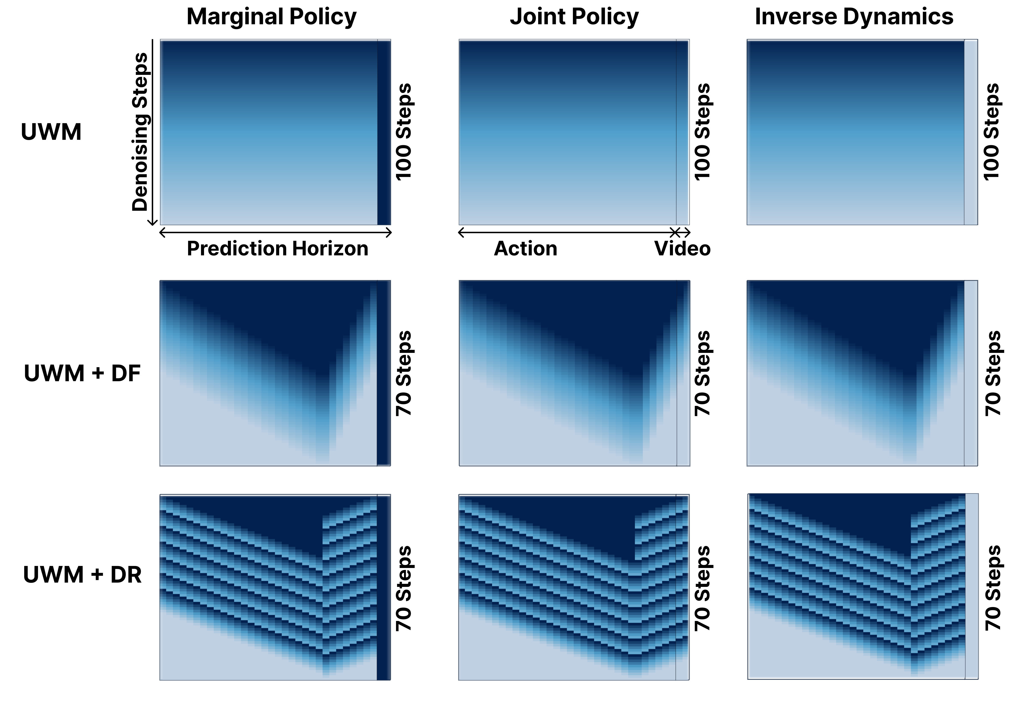
OOD evaluation expands object-position initialization by ±0.03 m and removes task-irrelevant background objects. Action-only mode leaves future-image tokens at full noise; inverse dynamics conditions on clean future frames; joint mode generates both modalities. The modes therefore differ in available information.
Joint horizon and action-execution protocol.
The horizon contains 32 actions and two future frames, extended from the original UWM’s 16 actions. Obs./Hor./Act.=2/32/32 executes all 32 actions before the next prediction. Comparable generated examples use 100 UWM DDIM steps versus 70 DF/DR schedule updates.
Equation 23
| (23) |
Inverse dynamics setting.
Inverse dynamics starts from a demonstration initial state and conditions on future image pairs at steps (32,33), (64,65) and so on. Its budget is 32 times the integer floor of (demonstration length−2)/32, typically 128–512 actions, whereas policy evaluation allows 1,000. Success and cost cannot be compared across these modes as if their horizons and observations matched.
Equation 24
| (24) |
Asymmetric min-SNR clipping.
Action loss clips SNR at 2.5 and image loss at 5. Different clipping acknowledges different modality scales/noise sensitivity. The complete weighting formulas and corresponding hyperparameters are retained.
Image-loss weight.
Image reconstruction receives weight 1.5 relative to action loss in the reported configuration. This is a chosen training balance, not a learned proof of equal action/video importance.
Equation 25
| (25) |
C.4.2 Applied ReRoll Parameters
The meeting schedule uses six forward and nine reverse events, with a meeting point near 0.765 for the 34-token joint sequence and 0.75 for 32 actions. Slopes are about 3.78/3.56 and the reset threshold 0.412K. The nine matrices show how conditioning differs among marginal policy, joint policy and inverse dynamics.
| Parameter | Value |
| Joint horizon | 34 |
| Action horizon | 32 |
| Meeting point | / |
| Denoising slope | / |
| ReRoll events, forward | 6 |
| ReRoll events, backward | 9 |
| Reset noise level | |
| Training chunk count | – |
| Chunk slope range | |
| Starting-level range | |
| Bidirectional branch probability | 0.30 |
| Full-horizon branch probability | 0.05 |
| Image-inpainting probability | 0.1 |
C.4.3 Basic Learning Hyperparameters
The full table records pretraining/fine-tuning optimization, modality losses, noise schedules, patching and architecture. Comparisons share data and settings where possible, but token-level conditioning requires the interface changes described in Appendix B.4. Reported standard deviations cover fine-tuning seeds only.
| Hyperparameter | UWM | UWM + DF / DR |
| Backbone | DiT-style joint transformer | DiT-style joint transformer |
| Embedding dimension | 768 | 768 |
| Depth / heads / MLP ratio | 12 / 12 / 4 | 12 / 12 / 4 |
| Register tokens | 24 | 24 |
| Image latent patch shape | ||
| Positional embedding | learnable | sinusoidal |
| Noise conditioning | global AdaLN | per-token input concat. |
| Optimizer | AdamW | AdamW |
| , | , | , |
| Learning rate, pretrain | ||
| Learning rate, finetune | , cosine, 1k warmup | , cosine, 1k warmup |
| Weight decay | ||
| Pretraining steps | ||
| Fine-tuning steps | ||
| Batch size, train / eval | 16 / 4 | 16 / 4 |
| Observation history | 2 | 2 |
| Visual backbone | ResNet | ResNet |
| Image resize / crop | / | / |
C.5 Real-World Navigation
The physical navigation experiment evaluates a learned visual waypoint generator and fixed learned inverse-dynamics controller on one obstacle course. Both complete circuits and four constituent subtasks are reported.
C.5.1 Evaluation Environment Settings
A Jackal with an onboard RTX 3060 follows black drivable regions among colored blocks and movable obstacles. Distribution shifts change objects, floor configuration and illumination. All methods share the demonstrations, inverse controller and physical test layout.
Evaluation protocol.
Three independently trained policies each run three circuit trials per direction and five trials per subtask. Thus a direction has nine trials across seeds and a subtask fifteen; the four subtasks are portions of the same course rather than independent environments. Per-seed results are shown in the main figure.
Failure criteria.
A collision fails only if it prevents progress or moves an obstacle more than 3 cm; minor contact is allowed. Leaving the drivable area fails when more than half the robot footprint crosses the black boundary. Most boundary failures are clear departures, and these operational criteria qualify the meaning of success.
Demonstrations.
Approximately 40 minutes comprise ten recordings, five per direction, with changing obstacles. A shared 90/10 train/validation split is used for all methods and seeds. Future targets are sampled at 5 Hz. This is a compact, course-specific dataset.
Observations and control.
One 320×240 RGB frame conditions sixteen waypoints at 0.2-second spacing, expressed relative to the current robot frame with position and yaw sine/cosine. The first eight form a 1.6-second planning prefix, which one MLP maps to a single linear/angular velocity command. Updating at 5 Hz does not execute eight waypoint actions open loop.

C.5.2 Applied ReRoll Parameters
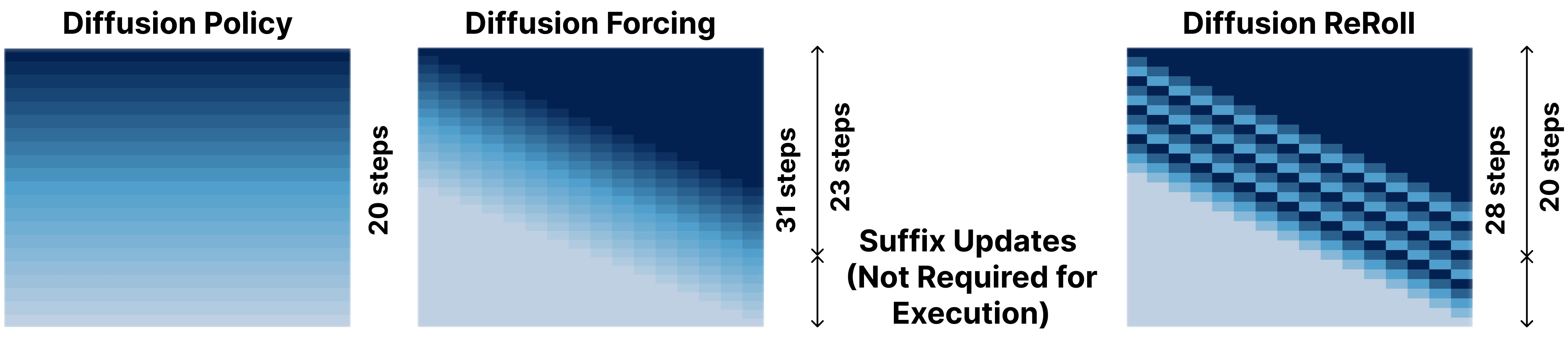
DR uses three waves, slope four and reset threshold 0.5K. DF and DR stop when the first eight waypoints are clean: DP uses 20 DDIM updates, DF 23 deployed schedule updates and DR 20. The complete DR matrix is longer, but the controller never needs its unresolved suffix.
| Parameter | Value |
| Prediction horizon | 16 waypoints |
| Prefix supplied to inverse dynamics | 8 waypoints |
| Denoising slope | 4 |
| ReRoll events | 3 |
| Reset trigger level | |
| Training chunk count | 1–8 |
| Training chunk slope range | |
| Noninitial chunk starting-level range | |
| Deployed updates, DP / DF / DR | 20 / 23 / 20 |
C.5.3 Basic Learning Hyperparameters
Navigation uses the same modified Transformer and pretrained ResNet-50 across the policy comparisons, plus a separately fitted inverse-dynamics MLP. The original tables retain architecture and training values.
Diffusion training.
All policy methods use a squared-cosine noise schedule. DP samples one shared token noise level, DF independent token levels and DR random linear chunks. DF/DR predict clean targets with min-SNR clipping 2.5; the visual encoder is fine-tuned jointly with the policy.
Data preprocessing.
Brightness, contrast and saturation each vary by strength 0.2, followed by ImageNet normalization. Waypoint positions are min-max normalized to [−1,1] during training and restored to metric units for control; yaw is represented by sine and cosine.
Inverse dynamics.
The inverse model flattens eight future waypoints, applies a ReLU MLP and predicts velocity commands, without current velocity/yaw-rate inputs. It fits ten demonstration recordings and validates on two separately recorded sequences. Its validation criterion and Smooth L1 loss differ from the policy’s open-loop waypoint error.
| Hyperparameter | Navigation policies | Inverse dynamics |
| Backbone | Modified Chi-Transformer | MLP |
| Visual encoder | Pretrained ResNet-50 | — |
| Hidden dimension | 256 | 256 |
| Decoder / hidden layers | 8 | 3 |
| Attention heads | 4 | — |
| Feed-forward dimension | 1024 | — |
| Noise embedding dimension | 128 | — |
| Dropout | 0.01 | 0.1 |
| Optimizer | AdamW | AdamW |
| Peak learning rate | ||
| Weight decay | ||
| Warmup | 5 epochs | None |
| LR schedule after warmup | Cosine | Cosine |
| Minimum learning rate | ||
| Batch size | 64 | 32 |
| Training epochs | 300 | 100 |
| Gradient clipping norm | 1.0 | 1.0 |
| Training diffusion steps | 100 | — |
| Prediction target | Clean trajectory | Linear/angular velocity |
| Loss | MSE; method-specific weighting | Smooth L1, |
| Checkpoint selection | Full-horizon validation ADE | Validation loss |
Appendix D Additional Results
Additional results distinguish best single-seed checkpoints from main seed averages, analyze zero-action errors and reset variance, and retain all long-horizon denoising/video examples.
D.1 Best-Checkpoint Results
Tables 17–19 report the maximum success observed across seeds and evaluated checkpoints for each method/setting. They complement, but do not replace, the main means and standard deviations. Best-of-seed reporting should not be interpreted as typical-run performance.
| Mode | Method | AntMaze | PointMaze | ||||
| Giant | Large | Medium | Giant | Large | Medium | ||
| Guidance Replan | Diffuser | 17.2 | 46.8 | 70.0 | 32.0 | 31.6 | 47.2 |
| Forcing | 56.0 | 61.6 | 96.0 | 92.8 | 62.0 | 94.0 | |
| ReRoll | 87.6 | 71.2 | 98.4 | 100.0 | 78.4 | 99.2 | |
| Inpainting | Diffuser | 34.4 | 72.8 | 89.2 | 66.8 | 96.4 | 95.2 |
| Forcing | 75.6 | 68.0 | 91.2 | 96.4 | 97.6 | 94.4 | |
| ReRoll | 84.8 | 74.8 | 94.4 | 99.2 | 100.0 | 99.2 | |
| Method | LIBERO-10 Official (Obs./Hor./Act.) | LIBERO-10 Open (Obs./Hor./Act.) | ||||||||
| 2/16/8 | 2/32/16 | 2/64/16 | 4/32/16 | 8/32/16 | 2/16/8 | 2/32/16 | 2/64/16 | 4/32/16 | 8/32/16 | |
| Diff. Policy | 31.6 | 49.6 | 38.2 | 52.2 | 54.8 | 76.6 | 67.6 | 60.2 | 70.6 | 66.0 |
| Forcing | 47.2 | 50.8 | 46.0 | 65.4 | 65.0 | 69.4 | 61.4 | 62.0 | 71.6 | 77.8 |
| ReRoll | 68.8 | 59.4 | 67.8 | 76.6 | 73.8 | 85.0 | 77.8 | 71.8 | 83.8 | 83.8 |
| Method | CloseSingleDoor | CoffeePressButton | CoffeeServeMug | PnPCounterToSink (300 Demos) | ||||||||
| 2/32/16 | 2/64/16 | 4/32/16 | 2/32/16 | 2/64/16 | 4/32/16 | 2/32/16 | 2/64/16 | 4/32/16 | 2/32/16 | 2/64/16 | 4/32/16 | |
| Diff. Policy | 54.0 | 54.0 | 66.0 | 82.0 | 64.0 | 84.0 | 46.0 | 36.0 | 46.0 | 34.0 | 26.0 | 26.0 |
| Forcing | 66.0 | 70.0 | 68.0 | 88.0 | 72.0 | 94.0 | 42.0 | 46.0 | 40.0 | 34.0 | 30.0 | 38.0 |
| ReRoll | 74.0 | 66.0 | 70.0 | 90.0 | 88.0 | 90.0 | 46.0 | 40.0 | 38.0 | 32.0 | 36.0 | 32.0 |
D.2 Details for the Zero-Action Intervention
Set future actions to zero, generate future frames and apply inverse dynamics to those images. Terminal end-effector displacement measures inconsistency under this intervention. DR gives 0.3006 m versus 0.3283 for UWM, 0.3170 for DF and a 0.3510 m demonstration reference; its reduction is 0.0504 m, not near-zero motion. Ground-truth zero-action images still produce 0.2915 m with DR, exposing inverse-model bias in the diagnostic. Thus lower error supports relative consistency but does not isolate video physics or individual DR components.
Equation 26
| (26) |
| Evaluation setting | Dataset ref. | UWM | UWM + DF | UWM + DR |
| Successful demonstrations | – | – | – | |
| Gen. zero-act video Inv. Dyn. | – | |||
| GT zero-act video Inv. Dyn. | – |
D.3 High Variance in LIBERO-10 Official 2/16/8
At official reset 2/16/8, one DR seed scores 23.6% while the other two score 60.6% and 68.8%; all three are strong under open reset. This pattern is consistent with sensitivity to initial gripper distribution shift, especially for short horizons, but it does not establish a unique cause. From-scratch small-data training can add seed variation.
| Seed | Official | Open | ||||
| DP | DF | DR | DP | DF | DR | |
| 17 | 28.6 | 24.0 | 23.6 | 76.4 | 66.4 | 78.4 |
| 23 | 31.6 | 40.8 | 60.6 | 76.6 | 69.4 | 85.0 |
| 42 | 24.0 | 47.2 | 68.8 | 75.6 | 69.2 | 84.2 |
| Mean | 28.1 3.8 | 37.3 12.0 | 51.0 24.1 | 76.2 0.5 | 68.3 1.7 | 82.5 3.6 |
D.4 Execution-Length and Delay Ablations
Execution-length and delayed-action tests probe whether future refinement helps near-term actions and how robust the method is to stale observations. They provide supporting evidence, with tradeoffs in closed-loop responsiveness.
Execution length.
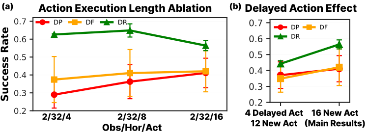
Holding observation history and prediction horizon fixed, DR remains best when executing four, eight or sixteen actions before replanning, with better success at four/eight than sixteen. This supports useful future context even when only a short prefix is consumed; it does not prove the mechanism independently of all other model differences.
Delayed actions.
Freeze four previously predicted actions, obtain the new observation before executing them, and predict twelve new actions conditioned on that fixed prefix; execute the combined sixteen. DR experiences the largest drop from delay, although its mean remains highest. Previously committed actions cannot be revised, illustrating why blocking latency and updated observations matter in deployment.
D.5 Long-Horizon Planning Visualization
The complete five-task, ten-stage denoising grids show full-sequence commitment, causal prefix errors and ReRoll route revision on AntMaze Giant. These are selected qualitative trajectories, not additional aggregate success measurements. All panels and step labels are preserved at native PDF fidelity.
D.6 Generated Video Visualization
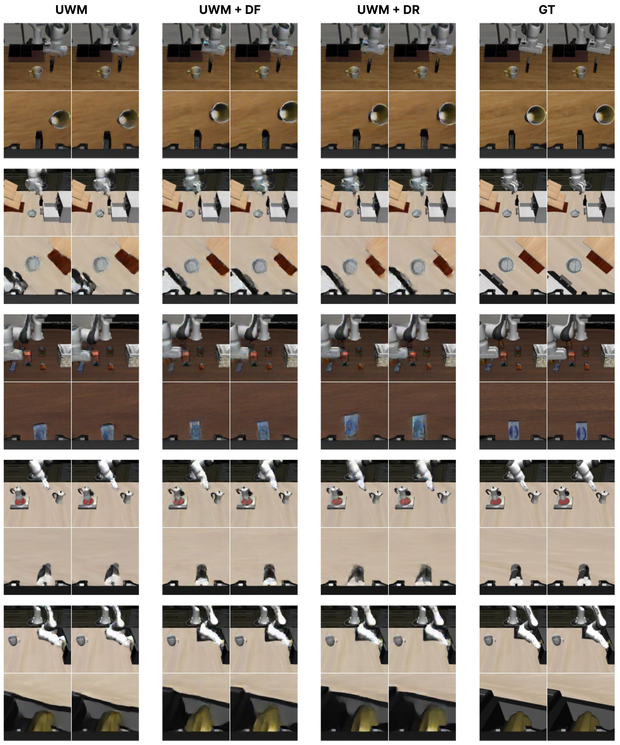
Two complete video grids compare UWM, DF, DR and ground truth. Visual quality is broadly comparable despite 100 versus 70 updates; the policy gains cannot be attributed merely to an obvious visual-quality advantage in these examples. No objective perceptual-quality metric is established by the selected grids.