Overview
This edition follows the 18-page arXiv v1 paper, including all five appendices. Its evidence concerns six tracked real objects, short training rollouts extended at evaluation, and small controlled manipulation studies. All original figures, tables, equations and 98 references remain; the figure artwork is restored from the PDF.

At a glance
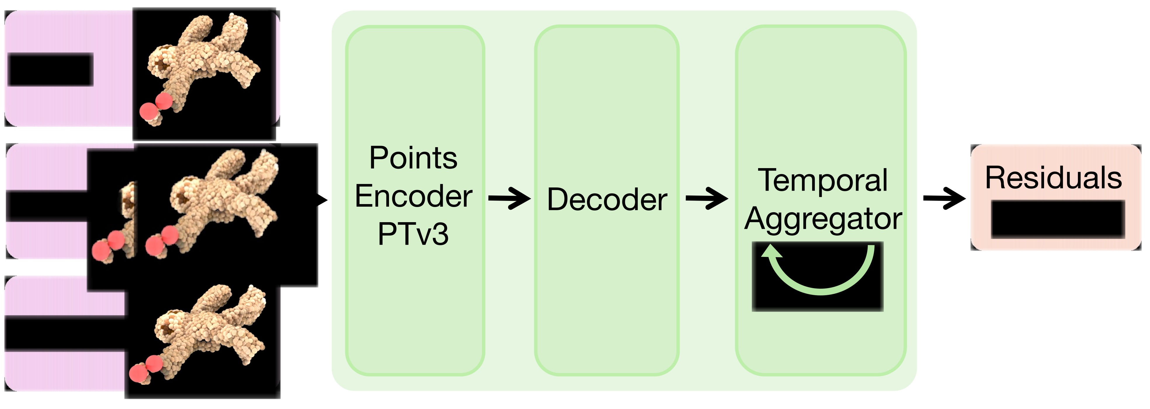
Physics-Guided Residual Dynamics (PGRD) first fits a spring–mass simulator, then learns corrections to its predicted velocities. A point-cloud encoder, position-conditioned decoder and gated temporal transformer improve tracked deformation and rendered-frame accuracy across rope, paper, flag, two soft toys and a duster. The model also drives predictive control and interactive Gaussian rendering; cable rerouting succeeds in 8/10 trials versus 2/10 for the fitted physics backbone.
I Introduction
Analytical simulators supply useful structure but imperfect materials, discretization and contact models leave systematic errors. Pure learned dynamics can fit those errors but require data and may drift. PGRD separates parameter fitting from residual learning so the backbone need not be differentiable. Velocity corrections are integrated into positions, and training recursively feeds back predicted states to expose the model to rollout errors. The evidence supports improved accuracy and empirical stability in the tested settings; this is not a conservation or stability theorem.
II Related Works
The paper relates spring–mass, finite-element, position-based and material-point simulators to learned graph/point-cloud dynamics. Differentiable simulators enable parameter identification but face difficult contact gradients; PGRD instead uses black-box fitting followed by learned corrections. Its closest comparison includes a custom differentiable spring–mass variant inspired by PhysTwin, and PGND as a learned point-based baseline. Hybrid modeling complements these approaches rather than eliminating their geometry and observation requirements.
III Method
The model has two training stages: optimize a small set of physical parameters against observed trajectories, then learn residual velocities on top of that fitted backbone. The following sections specify the simulator, corrected state update and temporally informed network.
III-A Physics Backbone
Particles are linked by springs and advanced with semi-implicit Euler integration. CMA-ES fits stiffness, damping, connection distance, maximum springs per node and ground friction. Grasped particles follow the gripper rigidly; non-prehensile interaction uses a spherical gripper collision model that projects penetrating particles to its surface. Volumetric toys receive internal particles from RaySt3R surface completion, a watertight marching-cubes mesh and interior sampling. This geometry prior helps prevent collapse but introduces reconstruction assumptions.
III-B Residual Dynamics Framework
The network adds a residual to the simulator velocity and the corresponding time-step-scaled correction to its position prediction. Corrections are zero on particles rigidly held by the gripper. Training minimizes mean squared particle-position error across autoregressive rollouts: each prediction becomes the next input. The model trains for five steps and is evaluated over 37, testing extension of rollout horizon. Directly correcting positions sometimes causes numerical divergence in the authors’ comparison; the velocity formulation improves this empirical behavior.
Equations 1
| (1) |
III-C Network Architecture
Point Transformer V3 encodes particle positions and velocities from the current/history states and the physics prediction. A Fourier-position-conditioned decoder predicts an initial three-dimensional velocity residual. A sliding-window transformer uses recent predictions, sinusoidal temporal encodings and repeated latest features when the buffer is not full. Its final projections produce a bounded correction and sigmoid gate. The retained formula blends the initial and temporal residuals and scales the entire blend by 0.1; it does not simply add an unrestricted temporal update. The appendix specifies layer sizes but does not give a numeric window length.
Equations
IV Experiments
Experiments compare predicted particle trajectories and object-only rendered video on six real objects. The paper also ablates the learned components and evaluates the simulator inside manipulation planning; the observation and split protocol matters when interpreting these results.
IV-A Data Collection
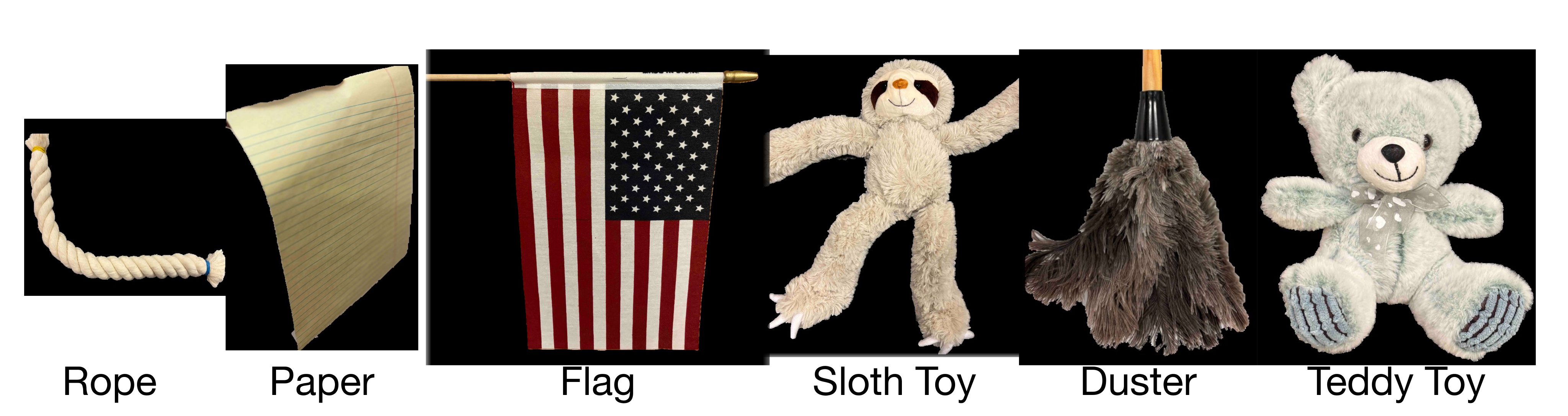
An xArm7 manipulates rope, paper, flag, sloth toy, duster and teddy toy, observed by four calibrated depth cameras. Most interactions are prehensile; the teddy is pushed, and the flag’s stick moves rigidly with the gripper. The reported collection protocol creates 100 training and 20 validation episodes of four seconds with a two-second stride: adjacent windows overlap. The unique recorded durations are 202 and 42 seconds, respectively. These windows should not be interpreted as 120 independent four-second trials; the paper does not fully specify their partitioning.
| Method | Metric | Rope | Paper | Flag | Sloth Toy | Duster | Teddy Toy |
|---|---|---|---|---|---|---|---|
| Spring-Mass [34] | MDE | ||||||
| MPM [73] | – | ||||||
| GBND [94] | |||||||
| PGND [93] | |||||||
| Diff. Spring-Mass [34] | |||||||
| Ours | |||||||
| Spring-Mass [34] | CD | ||||||
| MPM [73] | – | ||||||
| GBND [94] | |||||||
| PGND [93] | |||||||
| Diff. Spring-Mass [34] | |||||||
| Ours | |||||||
| Spring-Mass [34] | EMD | ||||||
| MPM [73] | – | ||||||
| GBND [94] | |||||||
| PGND [93] | |||||||
| Diff. Spring-Mass [34] | |||||||
| Ours | |||||||
IV-B Evaluation Tasks and Metrics
Particle evaluation uses correspondence-based mean distance error (MDE), bidirectional nearest-neighbor Chamfer Distance and Earth Mover’s Distance, reported in centimeters. Reference trajectories are reconstructed from image/depth tracking rather than directly instrumented particle positions. For video, Gaussians fitted to the initial observation follow predicted particle positions and covariances, while appearance remains fixed. Object-only overlap, boundary F-score and perceptual distance measure rendering; background pixels are ignored. Table II scales overlap and F-score by 10 and LPIPS by 100.
IV-C Baselines
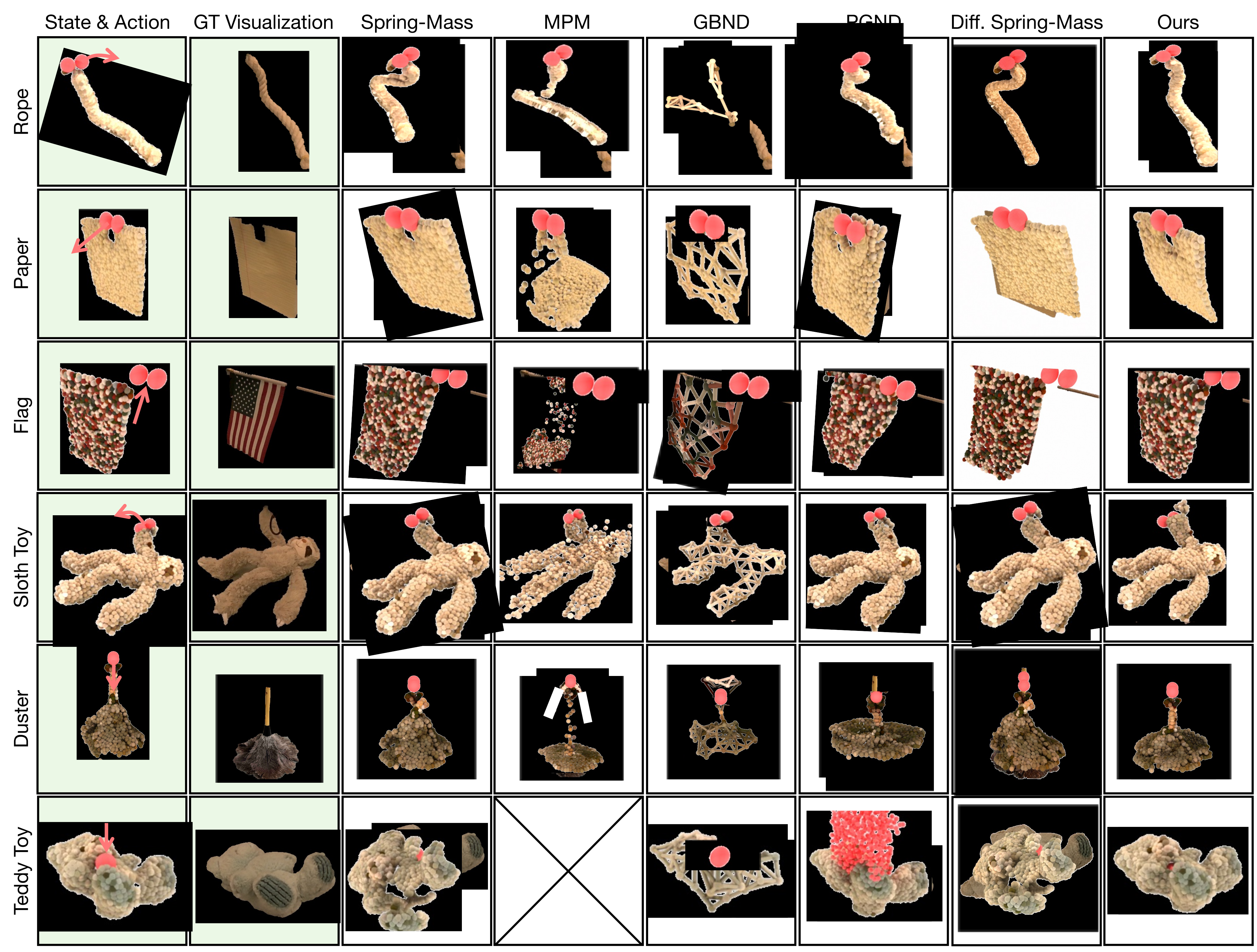
Five baselines are evaluated: fitted global spring–mass, Material Point Method (MPM), graph-based neural dynamics, PGND and differentiable spring–mass. The last is a PhysTwin-inspired implementation using a registered canonical spring graph, global fitting and spatial gradient refinement, rather than an unchanged PhysTwin system. The tested MPM implementation cannot handle the non-prehensile teddy interaction, so those entries are absent. Failure of this implementation on sparse thin objects does not establish a limitation of every MPM formulation.
IV-D Results
PGRD’s MDE means are 2.6, 1.7, 2.8, 2.7, 2.9 and 1.3 cm for rope, paper, flag, sloth, duster and teddy, versus 4.4, 2.3, 5.7, 3.2, 3.8 and 5.8 for global spring–mass. It gives the lowest reported means across the metrics, with a tie on flag Chamfer Distance. Qualitative comparisons show improvements for heterogeneous duster motion and teddy compression. The video table also favors PGRD’s mean overlap, boundary and perceptual scores. Reported uncertainty and some small margins preclude treating every comparison as established statistical dominance.

| Method | Metric | Rope | Paper | Flag | Sloth Toy | Duster | Teddy Toy |
|---|---|---|---|---|---|---|---|
| Spring-Mass [34] | -Score / IoU () | ||||||
| MPM [73] | – | ||||||
| GBND [94] | |||||||
| PGND [93] | |||||||
| Diff. Spring-Mass [34] | |||||||
| Ours | |||||||
| Spring-Mass [34] | -Score () | ||||||
| MPM [73] | – | ||||||
| GBND [94] | |||||||
| PGND [93] | |||||||
| Diff. Spring-Mass [34] | |||||||
| Ours | |||||||
| Spring-Mass [34] | LPIPS () | ||||||
| MPM [73] | – | ||||||
| GBND [94] | |||||||
| PGND [93] | |||||||
| Diff. Spring-Mass [34] | |||||||
| Ours | |||||||
V Applications
The fitted dynamics are used as a forward model for receding-horizon manipulation and as a motion model for interactive rendering. These applications reuse the learned object representation and calibrated observations.
V-A Planning using PGRD
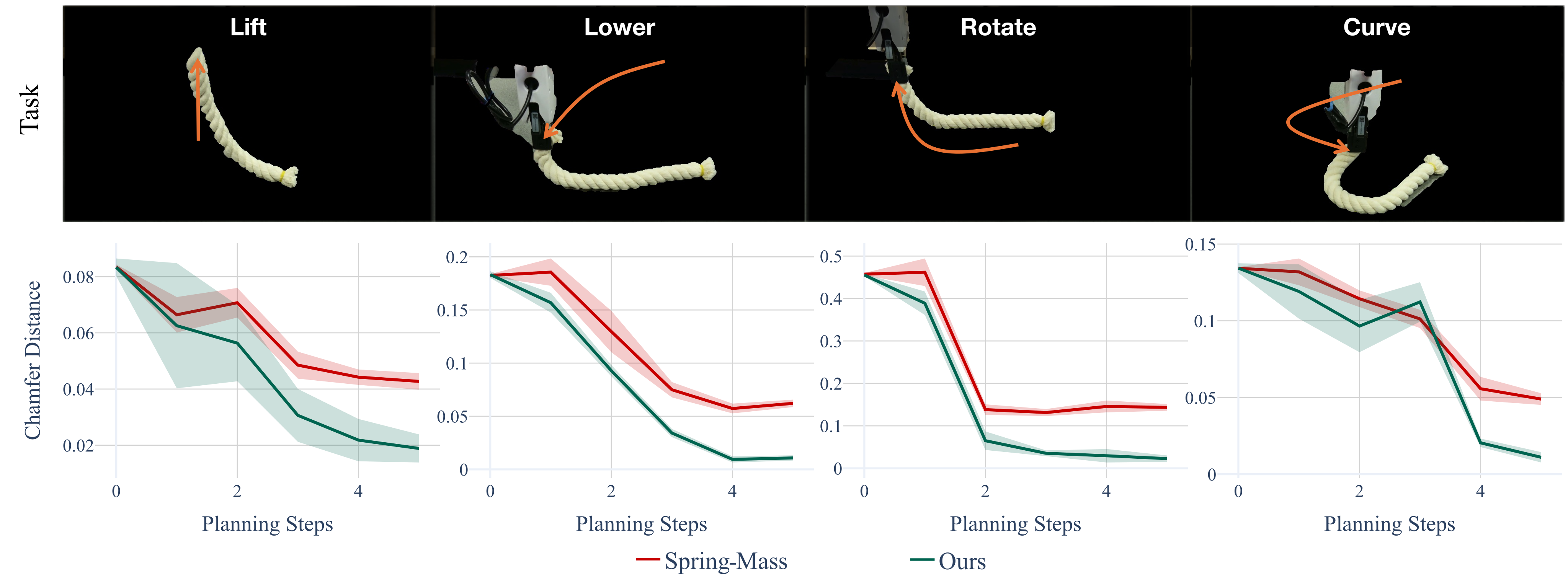
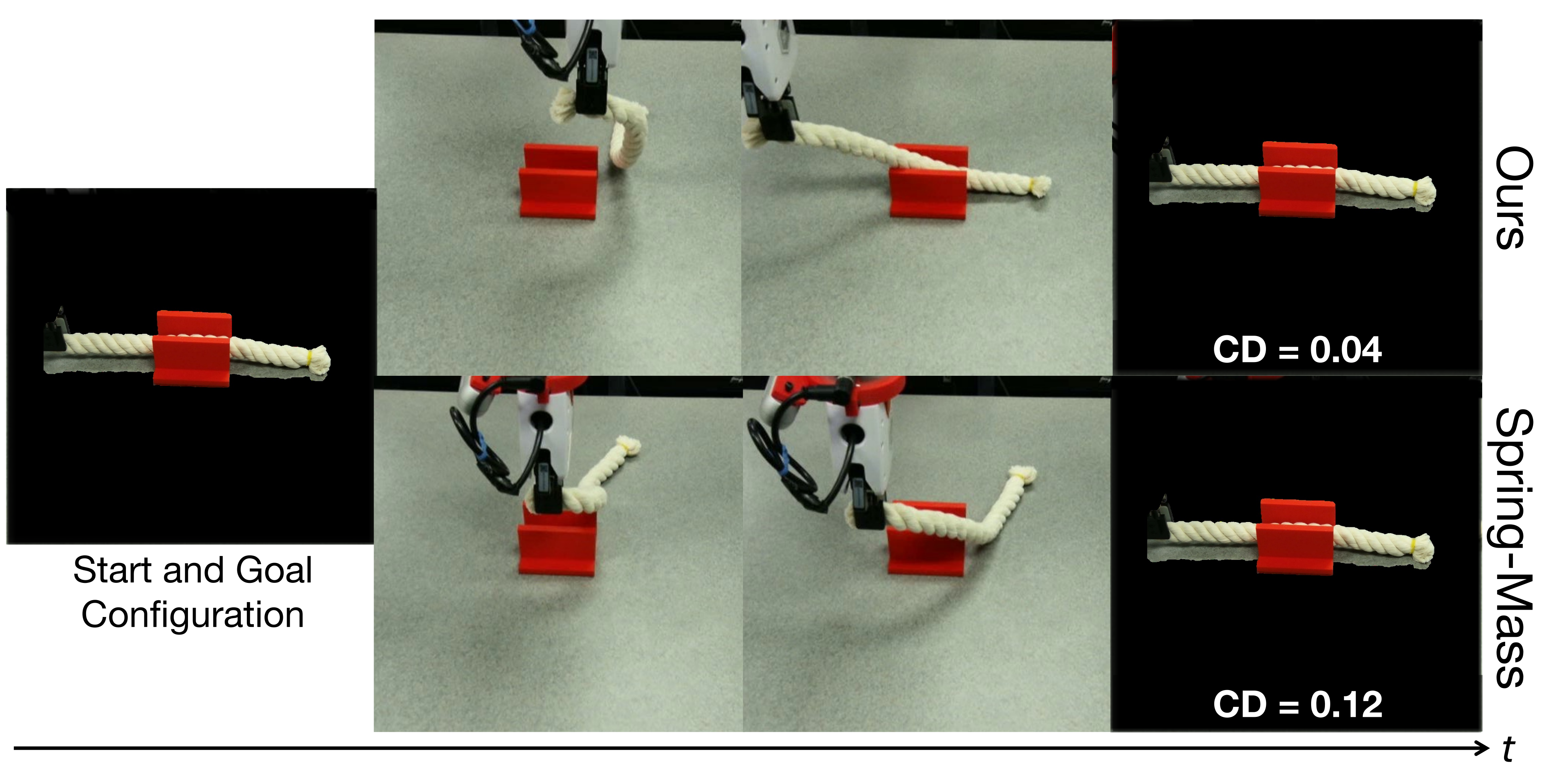
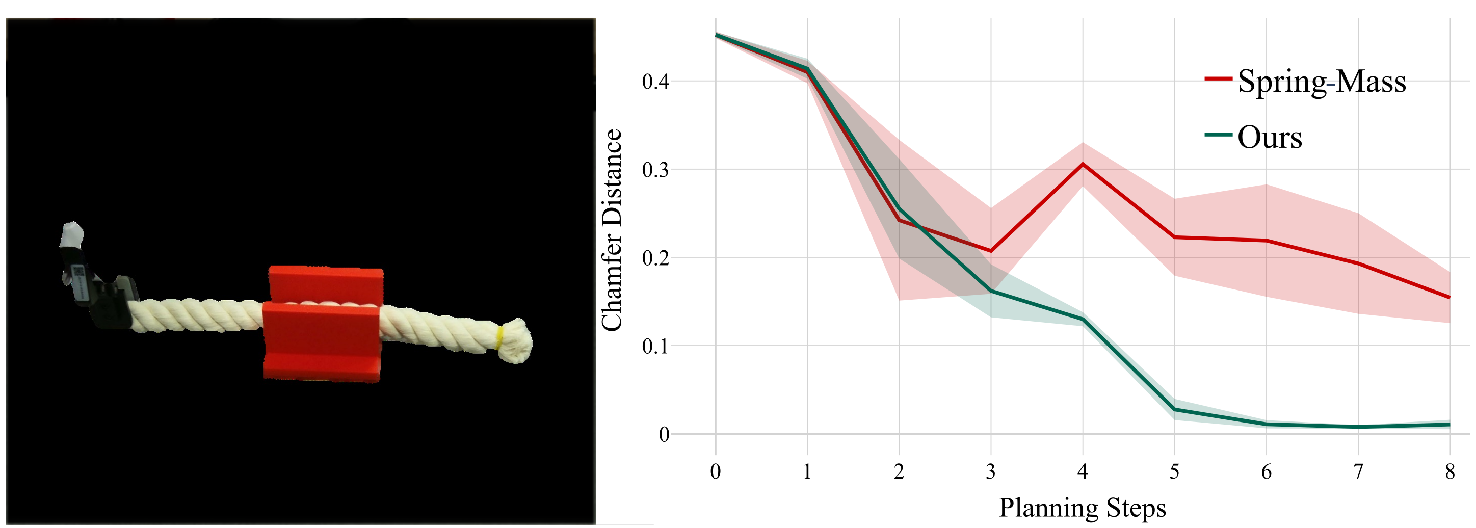
MPPI samples and refines action sequences using predicted Chamfer Distance to a target point cloud. Only the first action is executed before observing and replanning. Four rope objectives—lift, lower, rotate and curve—each receive ten trials with the same initial/goal states and equal planning budgets for PGRD and spring–mass. The curves demonstrate convergence in these matched settings rather than broad task success rates.
Cable rerouting uses ten varied start/end configurations and no rope–slot interaction examples in residual training. Success requires the entire rope to pass through the opening and the gripper to move below the final slot height: PGRD achieves 8/10 versus 2/10. This is a small, specific generalization test.
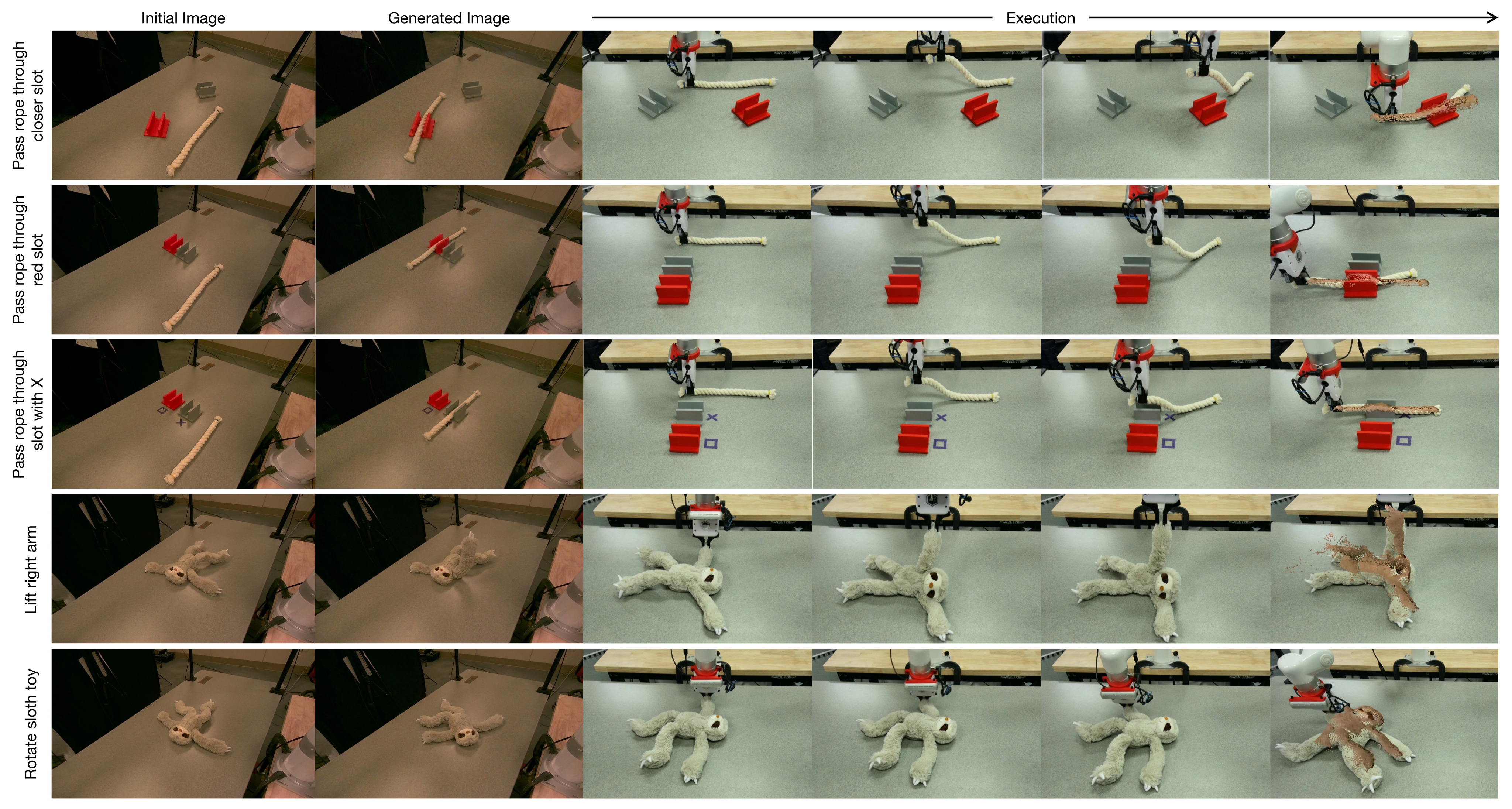
For language-conditioned goals, Nano Banana Pro edits an initial image; Depth Anything V2 estimates its depth, aligned affinely to the original depth using unchanged table points. Known camera intrinsics produce a target point cloud for MPPI. AnyGrasp supplies candidates: choose the rope’s right end, or use DINOv2 correspondences to identify the sloth region with largest requested motion. These single-camera demonstrations still depend on initial depth, calibration and generated-goal quality; no separate aggregate language-task success rate is reported.
V-B Interactive Photo-Realistic Simulation.
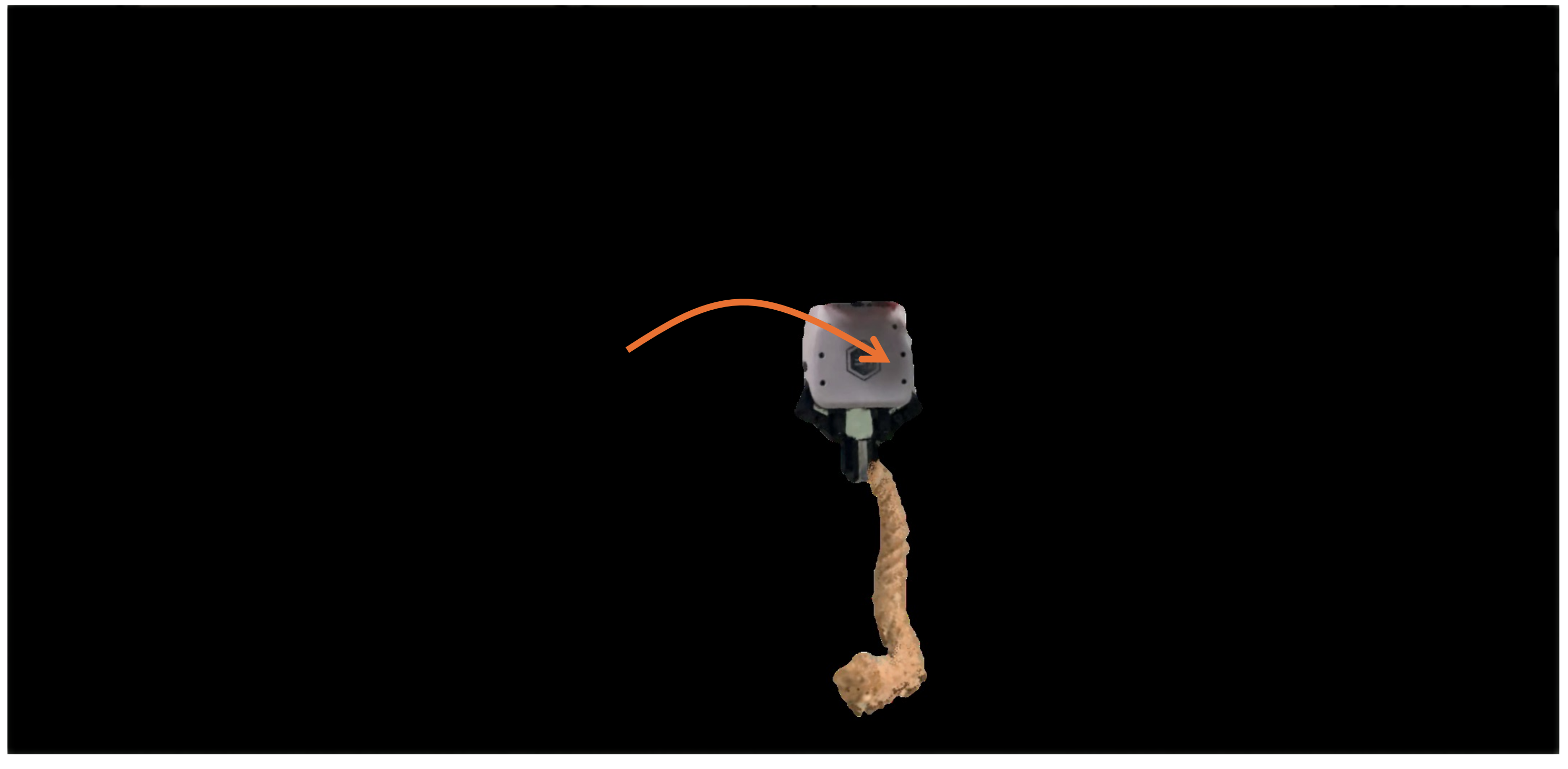
Keyboard manipulation commands drive the physics model and learned residuals, then particle motion updates Gaussian rendering. Fixed color/opacity retain the initial object appearance. The demonstration shows interactive action-conditioned deformation, without establishing generalization to new materials, lighting or arbitrary viewpoints, or reporting an inference-rate benchmark.
VI Conclusions
The central result is that a fitted physics backbone plus learned, temporally refined velocity corrections improves the tested real-object simulations and downstream planning. Limits include dependence on reconstructed geometry and tracked observations, object-specific training, short/small controlled evaluations and imperfect generated goals. Empirical rollout stability is useful evidence, but the formulation supplies no general conservation or stability guarantee.
A Ablation Study
Table III tests architectural alternatives on rope and sloth, reporting MDE. Full PGRD obtains 2.6/2.7 cm. These component ablations support the chosen combination in two objects rather than isolating universal design laws.
| Ablation variant | Rope | Sloth Toy |
|---|---|---|
| PGRD | 2.6 | 2.7 |
| Replace PTv3 with PointNet++ | 3.0 | 3.2 |
| Remove decoder | 2.8 | 3.0 |
| Remove temporal aggregator | 2.8 | 3.1 |
| Replace gating with addition | 2.7 | 2.9 |
| Remove internal particles | N/A | 3.8 |
A-A Encoder choice
Replacing PTv3 with PointNet++ raises rope/sloth MDE from 2.6/2.7 to 3.0/3.2 cm, supporting the stronger encoder for these residual-prediction tasks.
A-B Decoder
Directly projecting encoder features without the position-conditioned decoder raises MDE to 2.8/3.0 cm. Explicit spatial decoding remains helpful even after point-cloud encoding.
A-C Temporal aggregator
Removing temporal aggregation raises MDE to 2.8/3.1 cm. Recent motion history helps predict deformations that are ambiguous from a single configuration.
A-D Gated temporal refinement
Replacing the gate with direct addition gives 2.7/2.9 cm. The experiment supports controlled blending of temporal information; it does not prove that gating guarantees stable dynamics.
A-E Internal particles for volumetric objects
Removing interior particles raises sloth MDE to 3.8 cm; rope has no corresponding volumetric ablation. The qualitative rationale is that a surface-only spring network can collapse. The teddy also uses interior particles, but this table reports only sloth.
B Network Architecture Details
The encoder uses 18 input channels and 64-dimensional features. The conditional decoder has two hidden layers of width 64 and three velocity outputs. The temporal transformer has 64-dimensional embeddings, four heads, two layers and a 128-dimensional feedforward block; the final residual scale is 0.1. Table IV retains these settings exactly.
| Parameter | Value |
|---|---|
| Encoder (PTv3) | |
| Feature dimension | 64 |
| Input channels | 18 |
| Decoder | |
| Hidden layers | 2 |
| Hidden dimension | 64 |
| Output channels | 3 |
| Temporal Aggregator | |
| Embedding dimension () | 64 |
| Attention heads () | 4 |
| Transformer layers () | 2 |
| Feedforward dimension () | 128 |
| Gating scale | 0.1 |
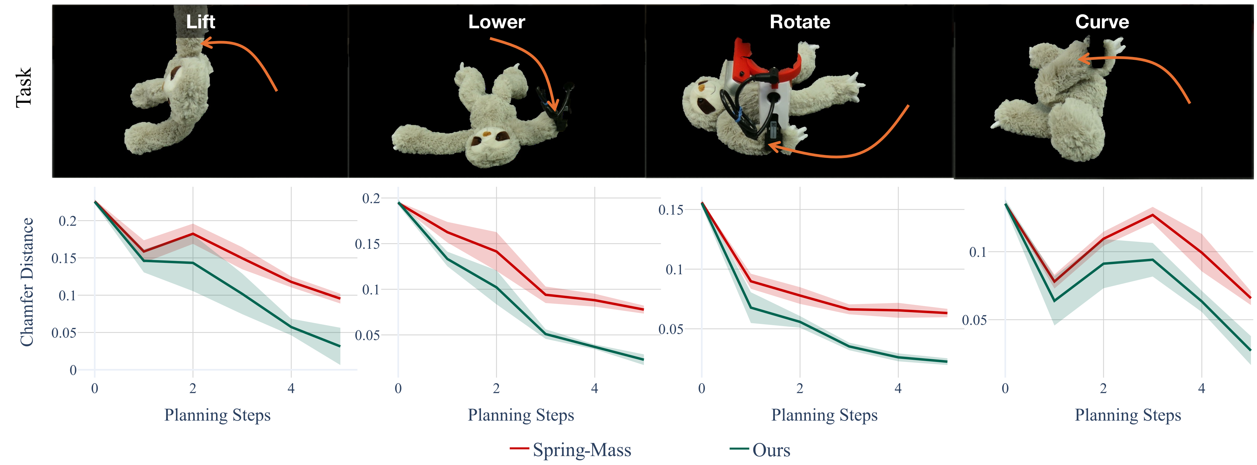
C Planning on Sloth Toy
Sloth planning repeats lift/lower/rotate/curve objectives, with ten trials each using identical start/target states and matched computational budgets. PGRD reduces target Chamfer Distance more consistently, while the spring–mass model may plateau on complex limb deformation. Figure 11 extends the convergence evidence to a volumetric toy, with the same limited-state trial design.
D Data Collection and Processing
Four RealSense D455 cameras record synchronized color/depth at 30 Hz. Grounded SAM 2 segments each object, CoTracker tracks image points, and depth plus camera calibration lift displacements into a shared three-dimensional frame. Overlapping views’ velocities are averaged. Persistent particles are propagated by their velocities, then updated from the mean velocity of their five nearest observed neighbors. The reported approximately 2 Hz for 1,000 particles describes this offline processing pipeline, not the dynamics model’s inference speed.
E MPPI Planning Parameters
Simple tasks use eight sampled trajectories, a ten-step horizon and three MPPI optimization iterations; rerouting uses 15 trajectories, a 15-step horizon and six iterations. Both use covariance 0.1. These budgets define the matched comparisons rather than a universal controller configuration.
| MPPI Hyperparameter | Simple tasks | Cable rerouting |
| Number of sampled trajectories | 8 | 15 |
| Planning horizon length | 10 | 15 |
| Optimization iterations per step | 3 | 6 |
| Action noise covariance | 0.1 | 0.1 |