Overview
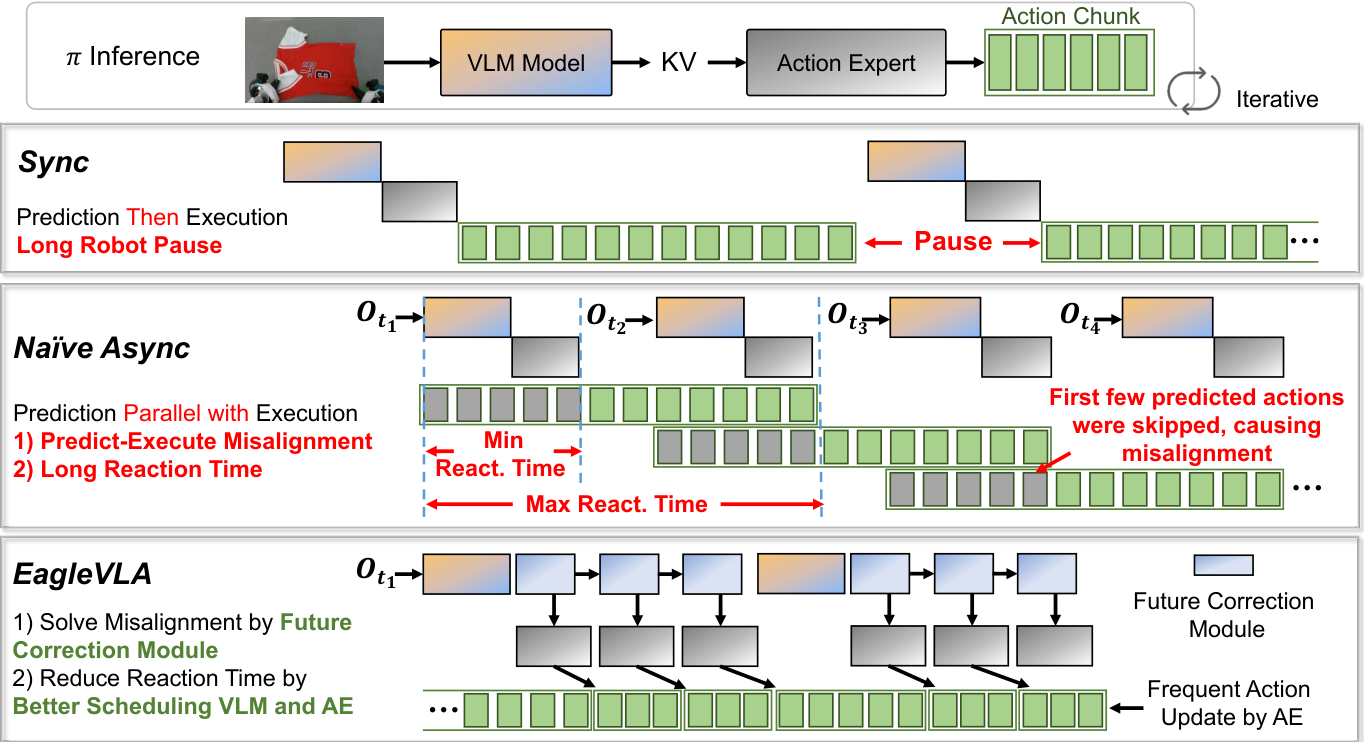
EagleVLA combines predicted future visual-language features, adaptive model scheduling, and an optimized onboard inference engine to improve asynchronous robot control.
| Parameter | Value |
|---|---|
| ViT (SigLIP So400m) | |
| ViT layers | 27 |
| ViT embedding dimension | 1152 |
| ViT patch size | 14 |
| Input Image Size | 224 |
| LLM (gemma 2b) | |
| LLM layers | 18 |
| LLM embedding dimension | 2048 |
| LLM attention heads | 8 |
| LLM head dimension | 256 |
| Action Expert (gemma 300m) | |
| Action expert layers | 18 |
| Action expert embedding dimension | 1024 |
| Action expert attention heads | 8 |
| Action expert head dimension | 256 |
| Denoising steps | 10 |
At a glance
A small correction model predicts the scene representation after already committed actions execute, helping the action expert compensate for inference delay. A learned confidence score schedules occasional full vision-language updates between cheaper action predictions. CUDA graph reuse, device-resident buffers, and denoising unrolling further accelerate execution. On Jetson Orin the reported action-update rate rises from 0.70 to 10.30 Hz, while a full visual-language-action pass still takes 271.1 ms. The faster update rate should therefore be distinguished from the rate of incorporating fresh camera observations.
1 Introduction
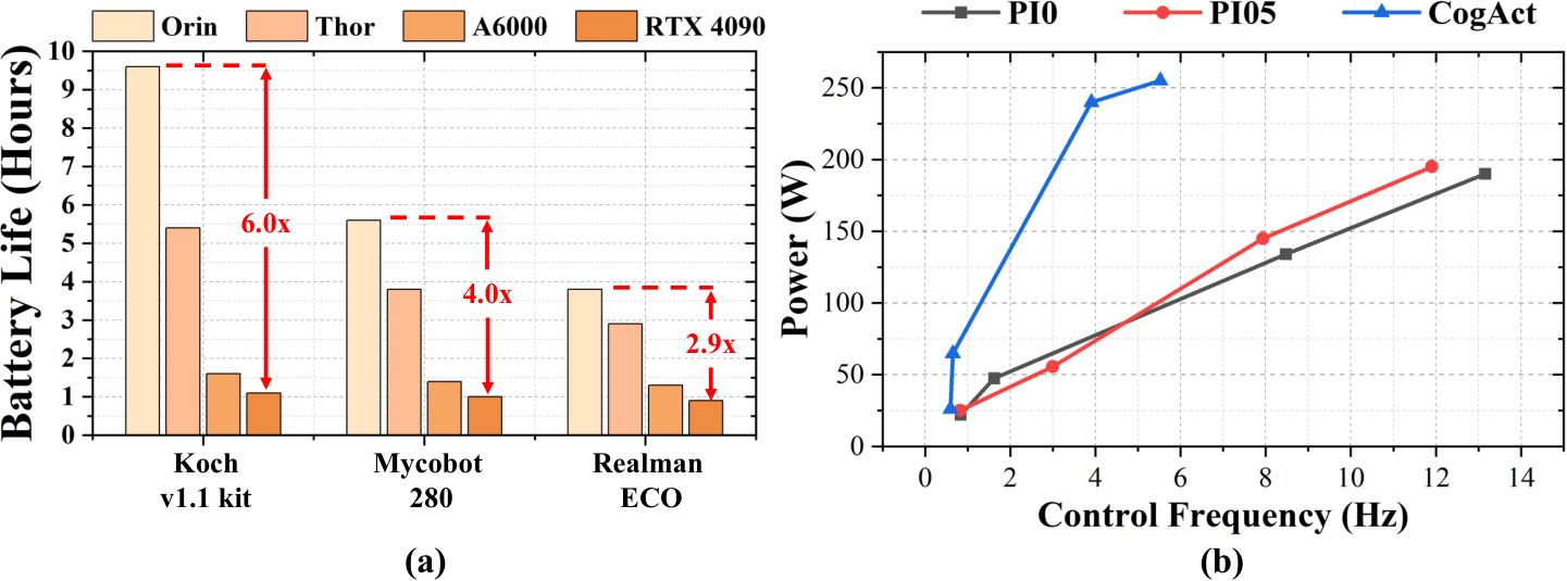
Onboard inference can take long enough that an action chunk is based on a scene that has changed before execution. Overlapping inference and action execution removes pauses but does not itself correct stale perception. EagleVLA, previously called Jetson-PI, predicts the effects of the committed actions in representation space, then allocates full visual processing only when its prediction is considered unreliable. The paper also compares power and a 500 Wh battery scenario including mechanical consumption; those scenario-dependent comparisons do not establish a universal robot endurance multiplier.
2 Background
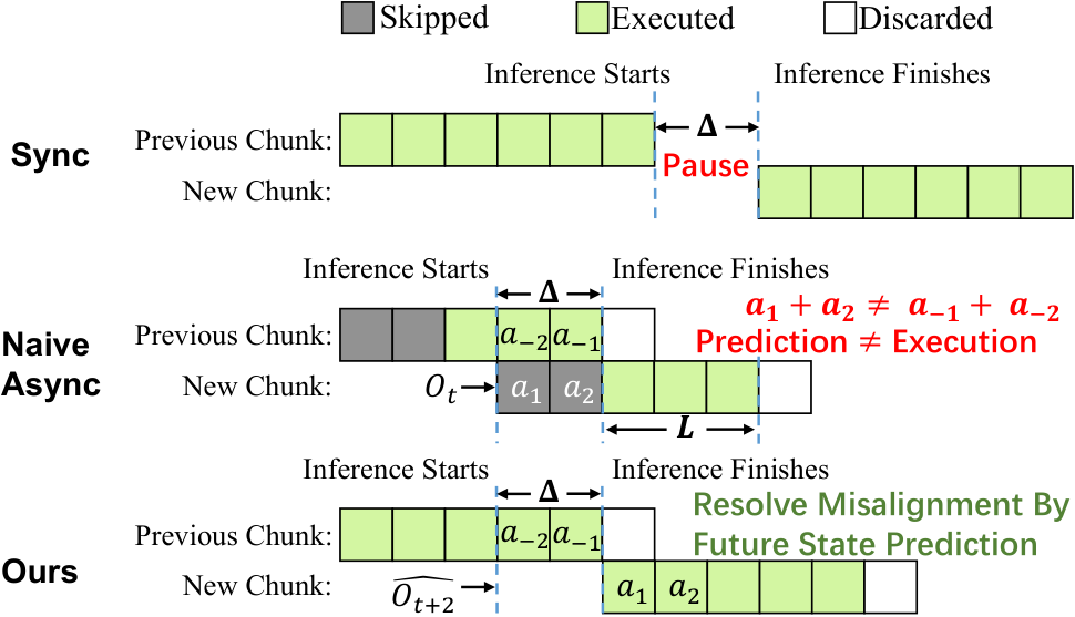
π₀.₅ [15] and related models pass vision-language key/value context to a flow-based action expert. real-time chunking [3] smooths asynchronous transitions by inpainting, while VLASH [35] uses predicted future robot state. EagleVLA additionally predicts environment features affected by committed actions. Its variable prediction horizon targets the time at which a newly inferred chunk begins, rather than a distant desired subgoal image.
3 When Asynchronous Inference Meets Onboard Computation
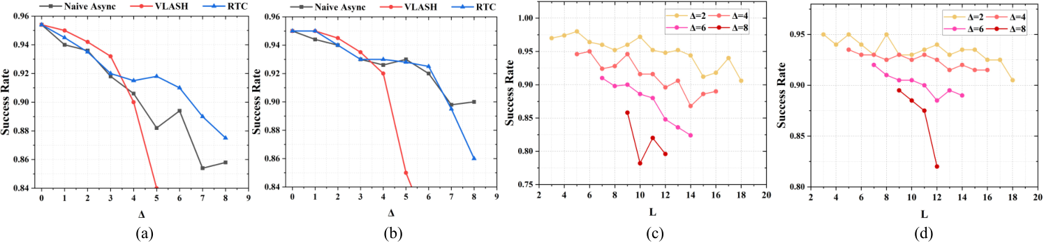
For a chunk executed over L steps and an inference delay of Δ steps, the paper analyzes response delays ranging from Δ to Δ+L. Longer chunks and stale inputs can reduce success. Continuous inference reduces gaps but remains limited by computation. EagleVLA addresses these issues jointly through future-state correction, selective visual-language invocation, and a more efficient execution engine. Feature prediction cannot reveal arbitrary external events that occur while fresh observations are skipped.
4 Method
The method comprises two-stage training of a future-feature correction model, confidence-driven scheduling, and system optimizations for fixed-shape VLA computation.
| VLA | Device | ViT | LLM | Action Expert | Total |
|---|---|---|---|---|---|
| Orin-30W | 322.4 | 856.4 | 1090.0 | 2268.8 | |
| Orin-50W | 152.5 | 632.3 | 518.2 | 1403.0 | |
| Thor | 63.7 | 185.0 | 199.2 | 447.9 | |
| A6000 | 23.4 | 43.5 | 46.9 | 116.1 | |
| 4090 | 13.1 | 32.2 | 22.4 | 69.5 | |
| Orin-30W | 329.0 | 858.2 | 1102.2 | 2289.4 | |
| Orin-50W | 152.3 | 631.0 | 536.8 | 1420.8 | |
| Thor | 61.7 | 187.0 | 209.2 | 457.9 | |
| A6000 | 23.8 | 51.2 | 50.2 | 128.2 | |
| 4090 | 13.2 | 35.9 | 25.2 | 76.4 |
4.1 Foresight-Aligned Asynchronous Correction
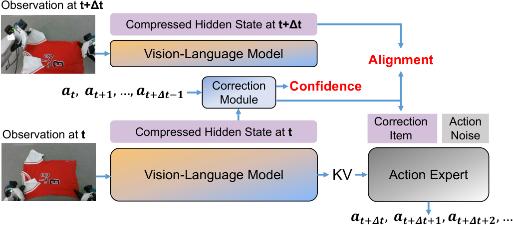
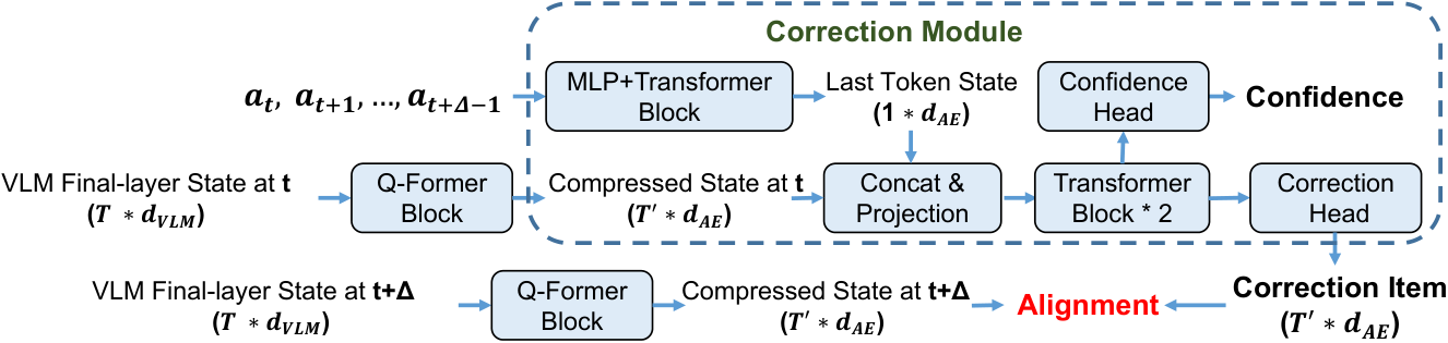
A roughly forty-million-parameter module receives compressed final-layer VLM features and the action prefix guaranteed to execute during the delay. It predicts compressed features at the future execution time; this correction supplements the action expert’s existing context rather than regenerating images or every layer’s cache.
Stage one trains the compressor and action expert using actual future features, teaching the expert to use the correction. Stage two learns to predict those features from current features and committed actions, sampling different delays during training. Its confidence head is trained toward the negative feature-prediction error, as shown in Equation 1. Confidence is therefore an error-related scalar with negative thresholds, not a calibrated probability of task success or safety.
Equation 1
| (1) |
4.2 Confidence-based Scheduling Optimization
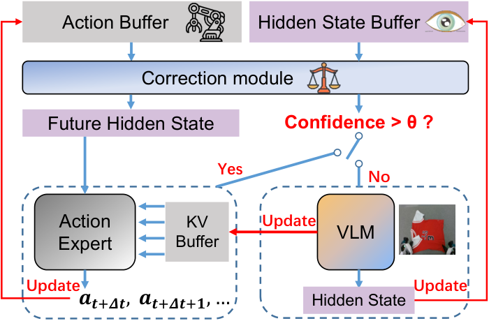
When predicted confidence exceeds a threshold, the scheduler reuses visual-language context and invokes the correction module plus action expert. Otherwise it captures the current scene, refreshes the VLM cache, predicts across the longer full-model delay, and updates the action buffer. Rolling predicted hidden states forward reduces computation but accumulates errors, motivating fresh observations.
The paper’s roofline argument attributes poor parallel VLM/action-expert execution on Jetson devices to shared memory-bandwidth contention. It therefore favors selective sequential invocation rather than simultaneous execution. This is an analysis of the tested models and devices, not a general prohibition on parallel edge inference. The original hardware specification and timing tables are retained for inspection.
| RTX 4090 | RTX A6000 | Orin 32GB | Orin 64GB | Thor | |
| Max Power (W) | 450 | 300 | 50 | 50 | 130 |
| TOPS | 309 | 309 | 200 | 275 | 510 |
| Memory | 24GB GDDR6X | 48GB GDDR6 | 48GB LPDDR5 | 48GB LPDDR5 | 48GB LPDDR5X |
| Bandwidth (GB/s) | 1024 | 768 | 204.8 | 204.8 | 273 |
| Balance Computational Intensity | 618 | 804 | 1953 | 2685 | 3736 |
| (TOPS/Bandwidth ) | |||||
| VLM | Compute Bound | Compute Bound | Bandwidth Bound | Bandwidth Bound | Bandwidth Bound |
| Action Expert | Bandwidth Bound | Bandwidth Bound | Bandwidth Bound | Bandwidth Bound | Bandwidth Bound |
4.3 System Design
Fixed image resolutions and padded language length allow repeated inference to reuse one CUDA graph. Fixed-size intermediate tensors remain in GPU buffers instead of returning through CPU memory. Multiple flow-denoising iterations are unrolled into one graph, trading a one-time construction cost for fewer repeated launches. These system changes preserve the modeled computation, but the complete method also requires correction-aware training and altered scheduling. They are complementary to quantization or pruning rather than substitutes for those techniques.
5 Experiments
Experiments test success under simulated delays, actual device latency, a physical clothes-handling task, and confidence-threshold behavior.
| SPATIAL | OBJECT | GOAL | LIBERO-10 | |||||||||||||
| Sync. | 97.3 | 99.6 | 96.7 | 93.5 | ||||||||||||
| VLASH | RTC | Ours | +Sched | VLASH | RTC | Ours | +Sched | VLASH | RTC | Ours | +Sched | VLASH | RTC | Ours | +Sched | |
| 1 | 98.8 | 97.1 | 97.7 | 98.6 | 99.2 | 98.5 | 98.7 | 98.8 | 96.7 | 96.5 | 97.0 | 97.5 | 94.4 | 92.3 | 93.4 | 93.1 |
| 2 | 97.5 | 95.4 | 97.1 | 97.6 | 99.2 | 98.5 | 98.5 | 99.3 | 97.0 | 96.0 | 96.2 | 97.3 | 94.6 | 92.1 | 92.7 | 92.9 |
| 3 | 94.4 | 94.5 | 97.1 | 97.2 | 98.8 | 96.4 | 98.2 | 98.4 | 93.3 | 94.3 | 96.7 | 96.4 | 91.9 | 89.6 | 91.3 | 91.9 |
| 4 | 92.5 | 92.5 | 96.7 | 96.9 | 96.9 | 97.7 | 97.8 | 98.9 | 93.3 | 93.3 | 95.9 | 96.9 | 89.6 | 85.8 | 91.8 | 92.3 |
| 5 | 84.3 | 91.2 | 95.9 | 96.7 | 94.3 | 96.9 | 96.9 | 98.6 | 89.9 | 93.9 | 96.0 | 96.1 | 80.3 | 83.6 | 91.5 | 92.0 |
| 6 | 74.4 | 91.7 | 97.0 | 97.5 | 88.5 | 97.4 | 98.3 | 98.4 | 81.3 | 94.0 | 96.7 | 96.9 | 78.5 | 84.6 | 92.2 | 92.9 |
| 7 | 51.3 | 91.7 | 97.0 | 97.3 | 81.4 | 97.1 | 98.0 | 98.4 | 76.1 | 92.6 | 97.1 | 97.2 | 77.0 | 85.3 | 92.6 | 92.6 |
| 8 | 46.7 | 90.9 | 97.2 | 97.5 | 65.1 | 93.8 | 98.3 | 98.8 | 70.8 | 93.4 | 96.8 | 96.8 | 65.5 | 83.2 | 92.3 | 92.7 |
| 9 | 30.1 | 88.8 | 97.0 | 97.3 | 51.7 | 93.1 | 97.5 | 97.6 | 59.7 | 92.5 | 96.3 | 96.5 | 59.6 | 81.0 | 92.0 | 92.2 |
| Avg | 74.4 | 92.6 | 97.0 | 97.4 | 86.1 | 96.6 | 98.0 | 98.6 | 84.2 | 94.1 | 96.5 | 96.8 | 81.3 | 86.4 | 92.2 | 92.5 |
| Jetson Orin | ||||||
|---|---|---|---|---|---|---|
| Method | ViT (ms) | LLM (ms) | Action Expert (ms) | Total (ms) | Reaction Time (ms) | Control Frequency (Hz) |
| Naive PI05 | 152.3 | 631.0 | 536.8 | 1420.8 | 1420.8 | 0.70 |
| +Schedule opt. | 152.3 | 631.0 | 536.8 | 1420.8 | 674.9 | 1.48 |
| +Graph reuse | 71.9 | 196.9 | 143.9 | 412.9 | 184.0 | 5.43 |
| +Intermediate Buffer & Unroll | 66.6 | 137.0 | 67.6 | 271.1 | 97.1 | 10.30 |
| Jetson Thor | ||||||
| Method | ViT (ms) | LLM (ms) | Action Expert (ms) | Total (ms) | Reaction Time (ms) | Control Frequency (Hz) |
| Naive PI05 | 61.7 | 187.0 | 209.2 | 457.9 | 457.9 | 2.18 |
| +Schedule opt. | 61.7 | 187.0 | 209.2 | 457.9 | 244.7 | 4.08 |
| +Graph reuse | 32.0 | 92.3 | 115.7 | 240.0 | 134.6 | 7.43 |
| +Intermediate Buffer & Unroll | 29.0 | 54.9 | 48.9 | 132.8 | 61.1 | 16.37 |
5.1 Simulation Experiments
Four LIBERO suites [21] compare a zero-delay synchronous reference, chunk inpainting, future-robot-state inference, feature correction, and correction plus scheduling. One trained correction model handles all tested Δ values from one to nine. The scheduler comparison estimates action-expert delay as the ceiling of one third of the full-model delay.
With scheduling, average success across suites and delays is about 96.3%, versus 81.5% for VLASH and 92.4% for chunk inpainting: gains of approximately 14.8 and 3.9 percentage points. At the largest delay, the respective gaps are 45.6 and 7.0 points. Small-delay VLASH results occasionally exceed EagleVLA, so the advantage is chiefly robust performance as delay grows. The zero-delay synchronous reference is a task-quality reference, not a realistic onboard latency baseline.
5.2 Latency Evaluation
On Orin, naive total inference is 1,420.8 ms at a reported 0.70 Hz update rate. Scheduling alone leaves full inference unchanged but reduces the reported reaction/update interval. With all system optimizations, a complete pass is 271.1 ms, the reported reaction interval is 97.1 ms, and the update rate is 10.30 Hz. These yield the stated 14.71-fold rate gain, while full-pass latency improves by about 5.24-fold.
On Thor, corresponding totals improve from 457.9 to 132.8 ms, with a reported 61.1 ms reaction interval and 16.37 Hz update rate. The 9.20-fold comparison to vla.cpp [25] uses its cited 893 ms Orin latency against EagleVLA’s scheduled update interval. These figures measure different invocation patterns; they do not mean a fresh camera-to-action forward pass runs at every high-rate update.

| Method | Picking | Folding | Placing |
|---|---|---|---|
| RTX 4090 (Baseline) | 10/10 | 7/10 | 10/10 |
| Jetson Orin (Naive Async) | 6/10 | 0/10 | 5/10 |
| EagleVLA (Ours) | 10/10 | 8/10 | 9/10 |
5.3 Real-world Experiments
A physical X2-W robot uses three 224×224 cameras, the XR-1 model on Orin, and 15 Hz action execution for cloth picking, folding, and placing. Each reported subtask has ten trials. EagleVLA scores 10/10, 8/10, and 9/10; the RTX 4090 reference scores 10/10, 7/10, and 10/10; naive Orin asynchronous execution scores 6/10, 0/10, and 5/10. These are subtask results, not a reported end-to-end success rate for the whole three-stage sequence. Fifteen-hertz actuator execution is also distinct from VLM observation refresh frequency.
5.4 Analysis of Confidence-Based Scheduling
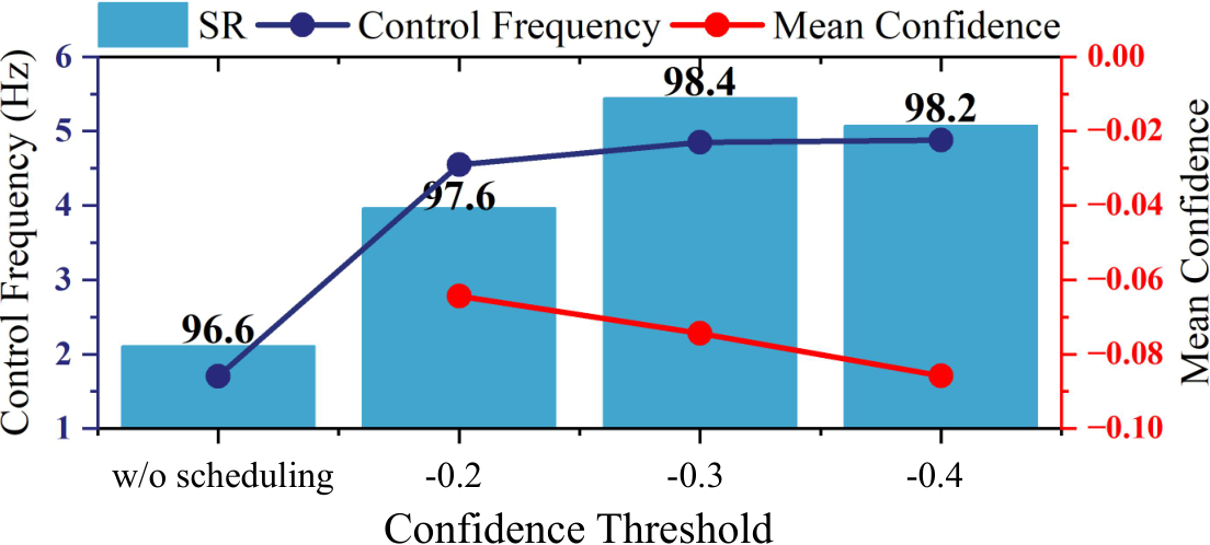
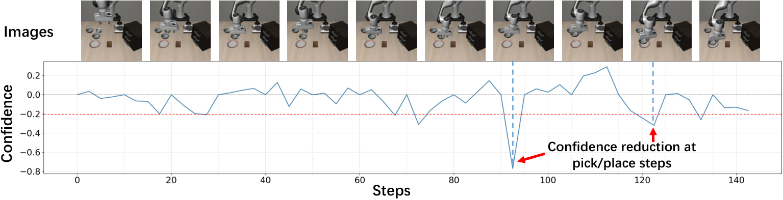
An example trace shows confidence dropping during difficult grasp/place transitions, triggering visual updates. A LIBERO-Spatial threshold sweep trades more frequent VLM calls against longer feature-only prediction periods. The tested thresholds improve reported success and update rate relative to no scheduling, but one trace and a threshold sweep do not establish confidence calibration or reliable detection of unseen external disturbances.
6 Conclusion
Future-feature correction helps an asynchronous action expert account for its own committed motion, while scheduling and graph-level optimizations substantially increase onboard action-update throughput. The strongest evidence combines delay-stress simulation, measured device inference, and a small physical cloth-handling evaluation. Fresh visual observation latency and task-level reliability remain distinct from the headline update rate.
7 Limitations
The paper identifies limited onboard compute and bandwidth as continuing constraints as model size and batch size grow. Its method also depends on predicted future features between visual refreshes; faster action-expert invocation does not supply new sensory evidence. The reported experiments do not establish general disturbance-response guarantees or long-duration battery performance across robot workloads.
8 Acknowledgments
The authors acknowledge support from national and municipal research programs in China, including work on efficient embodied-intelligence edge hardware.
Appendix A Model Architecture of π series Models
The model appendix specifies a twenty-seven-layer visual encoder, eighteen-layer language model, and eighteen-layer action expert with ten flow-denoising steps. Images and language generate key/value context used by the expert’s attention while action noise is refined into a chunk. EagleVLA adds predicted future hidden-state information to this pipeline. Table 5 retains all dimensions and head counts.
Appendix B Architecture of Future Correction Module
The committed action sequence is encoded by a multilayer network and transformer, retaining its final token. A Q-Former compresses VLM features to four tokens. Their joined representation passes through two transformer blocks and separates into a future-feature head and an error-related confidence head. Figure 10 preserves the exact dataflow and dimensions.
Appendix C Algorithm Details of Confidence-based Scheduling Optimization
Algorithm 1 maintains action, hidden-state, and key/value buffers while actions execute continuously. High confidence uses the shorter action-expert horizon and advances the predicted hidden state; low confidence observes the scene and refreshes context across the full-model horizon. The algorithm’s explicit observation step occurs only in the low-confidence branch, which is central to interpreting the throughput-versus-perception trade-off.
Appendix D Training Details
Both training stages use batch size thirty-two, AdamW, a 3×10⁻⁴ learning rate, cosine scheduling, and five hundred warmup steps on A100 hardware. Stage one uses thirty thousand steps and stage two twenty-five thousand. Table 6 retains the full reported configuration.