Overview
The author project page provides videos of the simulated and physical-robot experiments. This edition follows the paper’s reported protocols and retains its complete figures, tables, equations, and algorithms.
At a glance
A video-action model can imagine the right future yet execute the wrong action. This study measures that disconnect through Temporal Ratio (TR): action-token attention to predicted future frames relative to the current observation. Across controlled task recombinations, restricted backbone updates and partly denoised video features generalize better than several alternatives. An inference-time guidance rule uses changes in TR to strengthen language and longer-horizon conditioning during planning. Reported out-of-distribution success rises from 55.7% to 59.4% in simulation and from 71.7% to 83.3% in pooled real-robot trials. These are results for a particular model and evaluation setup, not evidence that attention measures reasoning or guarantees reliable plans.
1 Introduction
Video foundation models offer broad visual priors, but transferring them into robot control is an additional learning problem. Video-action models connect generated video features to an action policy; strong visual predictions alone do not establish that the policy uses those predictions. The paper calls this mismatch the video-action generalization (VAG) gap. [1] [8] [9]
The experiments recombine familiar objects, destinations, and instructions, distinguishing in-distribution (ID) execution from out-of-distribution (OOD) composition. A design sweep examines backbone adaptation, video noise, and prediction horizon. TR then supplies a diagnostic for how action attention shifts between current-state grounding and imagined futures, motivating adaptive inference guidance.
2 Design Space of Video-Action Models
The controlled architecture pairs a pretrained video generator with a flow-matching action head. Its design sweep changes the learned video representation and how that representation is queried at inference.
2.1 Background
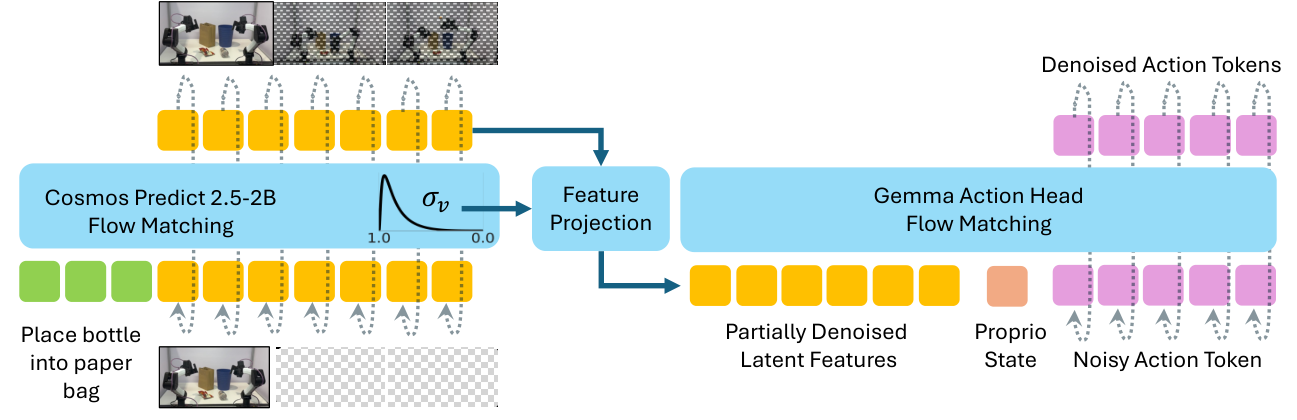
Cosmos-Predict 2.5 supplies a 28-block video DiT. The current image remains a clean anchor while future latent frames undergo denoising. Features from block 20, together with their video-noise level, condition a roughly 300-million-parameter Gemma action transformer. Proprioception and noisy action tokens complete its input. Separate flow-matching losses teach the video and action networks to predict their noise-to-data velocities. Language reaches the action head through video features rather than a separate text input. [1] [4] [38]
Equation 1
| (1) |
Equation 2
| (2) |
2.2 Design Axes
Training varies along two axes: LoRA versus full backbone finetuning, and joint video/action optimization versus video training followed by a frozen backbone and separately trained action head. Joint training allows action gradients to change video features. Inference varies the video denoising level and generated temporal horizon. The extended-horizon experiments still pass only the first five latent frames to the action head, keeping its input size fixed. [16]
3 Systematic Analysis of the Video-Action Generalization Gap
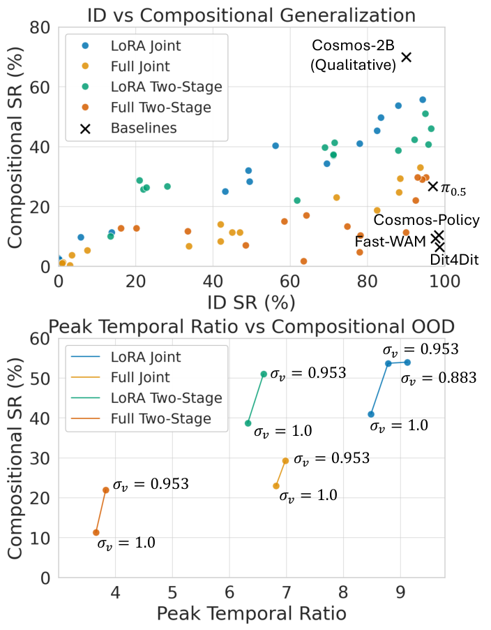
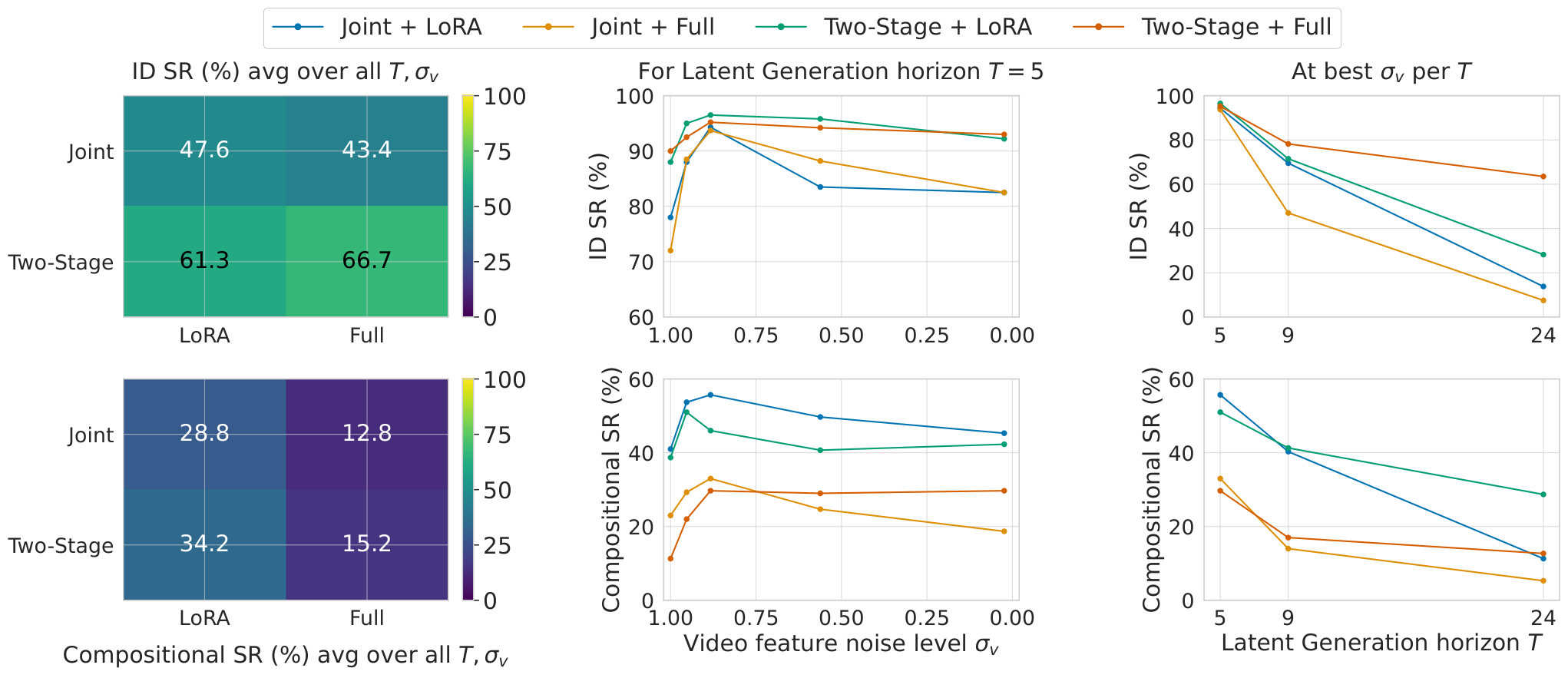
Generalization does not track ID success uniformly. Joint LoRA gives the strongest OOD configuration, while two-stage LoRA is more stable across the sweep. Features extracted before substantial denoising lack coherent future structure; nearly clean predictions can instead impose confident but incorrect trajectories. Intermediate noise performs best in the selected configuration.
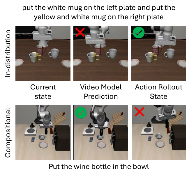
Longer videos can depict better object–goal relationships without improving actions. The examples show both directions of disagreement: an ID policy succeeds despite a mistaken predicted future, while an OOD policy ignores a correct future and repeats a familiar behavior. These observations motivate measuring the policy’s use of video features; they do not prove that visual prediction quality causes action success.
4 Understanding and Mitigating the VAG Gap via Temporal Ratio
TR sums head-averaged attention from action tokens to all future-video tokens and divides it by attention to current-frame tokens. The displayed equation defines the diagnostic at a selected action-transformer layer. TR is an attention-mass ratio, not a success probability or a causal explanation of the policy. Because the numerator covers multiple frames, its scale depends on the number of future tokens; equal per-token attention need not give a ratio of one.
Equation 3
| (3) |
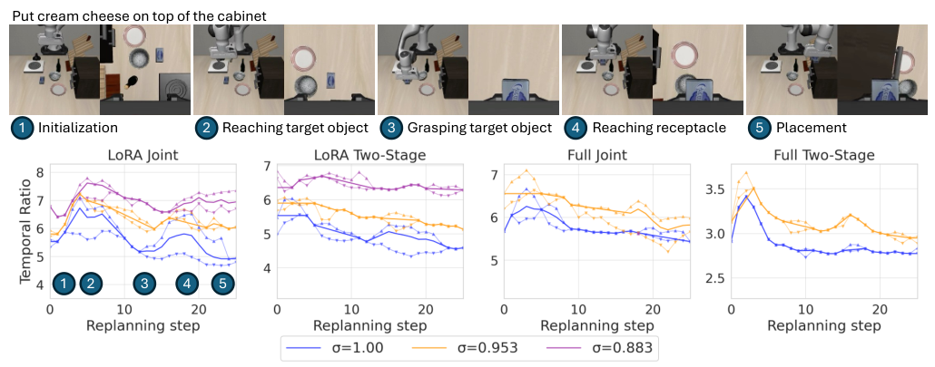
4.1 TR Analysis in Simulation: Key Findings
Denoising the video generally raises TR as future features become more structured. Within an episode, TR tends to rise during object or receptacle selection and fall during precise grasping or placement. Low TR can therefore be appropriate: close control needs current-state information. The proposed intervention responds to changes relative to an episode’s initial TR rather than maximizing future attention everywhere.
4.2 Adaptive TR Guidance
Two extra conditioning branches define guidance directions. Language guidance subtracts the action velocity obtained with a text-free video prediction from the conditional velocity. Plan guidance compares an extended video rollout with the ordinary rollout, truncating both to the same five-frame feature input. Their weighted differences modify each action-denoising update.
At each replan, TR is read on the first action-denoising step. A clipped increase relative to the first replan of that episode scales the guidance weights; they remain fixed for the rest of that action integration. Guidance turns off when TR does not exceed its baseline. This adds video and action-head evaluations whenever counterfactual branches are used; extracting TR from existing attention does not make the full intervention free.
5 Experimental Results
The evaluation combines controlled LIBERO recombinations with physical bimanual manipulation. The central comparison is the same policy with and without guidance. Baseline ID numbers come from prior papers where available; simulation OOD results use released checkpoints. Mimic-Video is omitted from OOD comparisons because its checkpoints are specialized to individual ID suites. Real-world baselines are retrained on the authors’ dataset with reported matched compute.
| In-Distribution | Out-of-Distribution | |||||||||
| Category | Method | Spatial | Object | Goal | Long | Avg ID | Spatial | Object | Goal | Avg OOD |
| VLA | 96.8 | 98.8 | 95.8 | 85.2 | 94.2 | 0.7 | 0.3 | 4.3 | 1.7 | |
| 98.8 | 98.2 | 98.0 | 92.4 | 96.9 | 36.7 | 2.3 | 41.7 | 26.8 | ||
| WAM/VAM | Cosmos-Policy | 98.1 | 100.0 | 98.2 | 97.6 | 98.5 | 30.7 | 0.3 | 0.7 | 10.5 |
| Fast-WAM | 98.2 | 100.0 | 97.0 | 95.2 | 97.6 | 12.7 | 0.0 | 15.7 | 9.4 | |
| Mimic-Video | 94.2 | 96.8 | 90.6 | – | – | – | – | – | – | |
| DiT4DiT | 98.4 | 99.6 | 98.6 | 97.6 | 98.6 | 9.0 | 0.0 | 10.3 | 6.4 | |
| Ours (best unguided) | 97.3 | 98.0 | 97.6 | 84.3 | 94.3 | 50.3 | 40.0 | 77.3 | 55.7 | |
| Ours (best guided) | 96.3 | 99.6 | 97.6 | 82.6 | 94.0 | 58.6 | 40.0 | 80.3 | 59.4 | |
5.1 Compositional generalization evaluation testbed
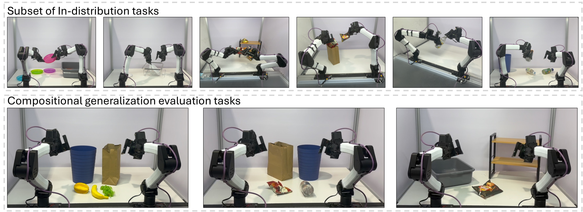
Simulation uses four ten-task ID suites, with 50 demonstrations per task, plus three ten-task OOD suites that recombine familiar objects, spatial relations, and destinations. A bimanual robot is trained on 24 tasks and 5,600 episodes, then tested on eight instructions across three scenes with multiple candidate objects and receptacles. These include both familiar and unseen bindings. [31] [17] [2]
5.2 Key Findings
Across four ID suites, unguided and guided average success is 94.3% and 94.0%. Across three OOD suites it is 55.7% and 59.4%, a 3.7-percentage-point increase. Spatial OOD improves from 50.3% to 58.6%, object OOD stays at 40.0%, and goal OOD rises from 77.3% to 80.3%. Guidance therefore does not improve every suite or preserve every ID result.
On the real robot, reported pooled success increases from 71.7% to 83.3%: 43 versus 50 successes under the stated 60-trial protocol. These are trial-weighted averages, not unweighted means over the eight tasks. Fully noisy video features reportedly fail on every real-world task, reinforcing the value of partially structured futures in this setup.
Only five trials are used for each of six real-world tasks; two fruit tasks receive 15 each. No uncertainty intervals are supplied. The authors report difficulty training their Cosmos-Policy implementation. Its tabulated percentage increments also do not match integer successes under the stated per-task trial counts, so that baseline requires particular caution.
| Method | Scene 1 | Scene 2 | Scene 3 | Avg | |||||
| Task 1 | Task 2 | Task 3 | Task 4 | Task 5 | Task 6 | Task 7 | Task 8 | ||
| 66.7 | 6.7 | 20.0 | 20.0 | 0.0 | 40.0 | 40.0 | 100.0 | 36.7 | |
| 80.0 | 20.0 | 100.0 | 40.0 | 20.0 | 20.0 | 100.0 | 80.0 | 55.0 | |
| Cosmos-Policy | 8.3 | 8.3 | 15.0 | 10.0 | 10.0 | 15.0 | 25.0 | 25.0 | 12.5 |
| Ours (unguided) | 80.0 | 53.3 | 100.0 | 60.0 | 40.0 | 100.0 | 100.0 | 60.0 | 71.7 |
| Ours (guided) | 80.0 | 73.3 | 100.0 | 80.0 | 80.0 | 100.0 | 100.0 | 80.0 | 83.3 |
6 Related Work
Prior work uses video prediction for planning, goal generation, feature extraction, and direct action generation. Video-action and world-action models differ in where video and action processing are coupled; strong pretrained visual representations do not settle how those representations are used for control. This paper complements architecture and pretraining advances with a diagnostic and inference intervention focused on compositional object–goal binding. [24] [32] [42] [45]
7 Conclusion
The study identifies video–action disagreement as a useful failure mode and shows that TR can help schedule guidance within the tested architecture. Its practical result is improved OOD execution with nearly unchanged aggregate ID performance, rather than a general solution to compositional robot control.
Limitations.
The evidence covers one video-backbone/action-head family and restricted task recombinations. TR may amplify unreliable future predictions, and attention patterns alone do not establish reasoning or causal reliance. Counterfactual guidance increases inference work; end-to-end latency is not reported. Real-world trial counts are small and one baseline’s training was unsuccessful.
Several reproduction details disagree within the source: simulation action-chunk length, full-finetuning learning rate, design-sweep evaluation totals, and real-world training schedules. The appendices below identify these discrepancies while retaining the original tables and pseudocode.
Appendix A Architecture and Algorithm Details
A.1 Latent VAM Architecture
The backbone produces a spatial-temporal feature sequence; the action transformer turns it into a denoising field over a future action chunk.
Video backbone.
The roughly 2.1-billion-parameter Cosmos backbone has 28 DiT blocks. Its VAE compresses time by four and each spatial axis by eight; latent patches and three-dimensional rotary position information represent the video. A mask identifies the observed anchor frame.
Action head.
The action expert has 18 layers, width 1,024, eight query heads, and one shared key/value head. GeGLU feed-forward layers and adaptive RMSNorm condition processing on action noise. Appendix A specifies bidirectional attention within the video prefix and among later action tokens, with causal state/first-action boundaries; the main text’s shorter description calls action attention causal.
Video-feature interface.
Selected video features are projected into action-head width and flattened across frames and spatial positions. A Fourier-based embedding of video noise modulates their interpretation. Proprioception and noisy action embeddings share the resulting token sequence.
A.2 Training and Inference Procedure
Training samples independent video and action noise levels. Joint optimization combines the two velocity losses; inference first constructs video features and then integrates the action flow.
Video denoising.
Video denoising stops at the selected feature-extraction noise level rather than necessarily producing a finished video. The current frame remains fixed while the future latent sequence is updated.
Action denoising.
Action generation uses ten Euler steps from Gaussian noise and executes an initial portion of the predicted chunk before replanning. Algorithms 1 and 2 retain the full training and unguided-inference procedures, including noise sampling, feature conditioning, and joint gradients.
First-frame anchor mechanism during video denoising.
The first-frame constraint combines a mask channel with explicit clean-latent replacement. Its velocity is replaced analytically to prevent corruption during integration; an optional near-zero anchor timestep is also described. The action head thus receives a stable current observation alongside imagined futures.
A.3 TR-Adaptive Guidance Algorithm
Algorithm 3 gives the complete adaptive procedure: reset the TR baseline each episode, compute guidance weights once per replan, and reuse conditional, text-free, and extended-plan features through action integration. Extended-plan features are truncated to the ordinary horizon. Only branches with active guidance weights need their counterfactual action evaluations.
Appendix B Simulation Task Setup
B.1 LIBERO In-Distribution Suites
The simulation setup uses the four original LIBERO suites and three additional suites designed to isolate compositional changes.
Suite definitions.
Spatial, Object, Goal, and Long each contain ten ID tasks. Three ten-task OOD suites change placement, manipulated object, or target goal while keeping the tested concepts individually familiar.
Training demonstrations.
Each ID task supplies 50 demonstrations. Action training uses the supplied filtered demonstrations. Main-text implementation notes distinguish filtered action data from unfiltered video data, while Appendix B describes filtering more generally; the exact backbone-data filtering convention is not fully consistent.
Evaluation protocol.
Main comparisons use 50 trials per task over three seeds: 1,500 trials per ten-task suite and 10,500 across seven suites. The design-sweep description instead gives ten trials per task and three seeds but a 700-trial total; those stated factors would produce 2,100 across seven suites. The original budget table is retained.
| Suite | Dist. | Tasks | Ep./task | Seeds | Total ep. |
| Spatial | ID | 10 | 50 | 3 | 1500 |
| Object | ID | 10 | 50 | 3 | 1500 |
| Goal | ID | 10 | 50 | 3 | 1500 |
| Long | ID | 10 | 50 | 3 | 1500 |
| Spatial-OOD | OOD | 10 | 50 | 3 | 1500 |
| Object-OOD | OOD | 10 | 50 | 3 | 1500 |
| Goal-OOD | OOD | 10 | 50 | 3 | 1500 |
| Total per config. | 70 | – | 3 | 10500 | |
B.2 LIBERO Compositional OOD Suites
The OOD construction changes task bindings rather than introducing unrestricted visual, embodiment, or dynamics shifts.
Spatial-OOD (object axis).
Spatial OOD combines four new pick-target bindings with a familiar plate and six familiar-bowl tasks using spatial relations absent from the ID task set. The relation vocabulary remains familiar; this is broader than simply swapping object positions.
Object-OOD (identity axis).
Object OOD keeps task names, scene layout, positions, and goal predicates fixed while swapping object-type bindings between named instances. All ten object classes participate. The policy must ground the instruction in the object’s current appearance rather than a memorized position-to-name association.
Goal-OOD (composition axis).
Goal OOD retains the object and changes its destination to another familiar receptacle, testing object–goal recombination rather than a fixed object-to-container association.
B.3 Relation to Other LIBERO Extensions
These suites target compositional binding. They complement broader LIBERO evaluations that change appearance, distractors, or scene configuration; performance here should not be read as robustness to every distribution shift.
Appendix C Design-Space Analysis and Additional Results
C.1 Full Training, Noise-Level, and Horizon Sweep
The complete sweep separates backbone adaptation, training coupling, extraction noise, and generated horizon. The best settings for familiar tasks need not be best for new combinations.
Finetuning strategy.
LoRA gives much stronger OOD results overall, although it does not improve every individual sweep cell. Joint LoRA reaches 55.7% OOD success; two-stage LoRA reaches 51.0%. The best tabulated full-finetuning OOD results are 33.0% for joint training and 29.7% for two-stage training; the latter differs from the appendix prose’s stated 33%.
Video noise level.
For joint LoRA at a five-latent-frame horizon, extraction at noise 0.883 gives 94.3% ID and 55.7% OOD success. Fully noisy extraction gives 78.0% and 41.0%; nearly clean extraction at 0.024 gives 82.5% and 45.3%. The intermediate optimum is configuration-dependent, not a universal noise threshold.
Prediction horizon.
Generated horizons of five, nine, and 24 latent frames correspond to 17, 33, and 93 decoded frames. The action head always consumes the first five latent frames. At noise 0.883, joint LoRA drops to 49.2% ID/32.0% OOD with nine generated frames and 0.0%/2.7% with 24. Longer generation changes the features without automatically yielding usable control.
| Paradigm | Horizon | ID | OOD | ID | OOD | ID | OOD | ID | OOD | ID | OOD |
| Joint + LoRA | 78.0 | 41.0 | 88.0 | 53.7 | 94.3 | 55.7 | 83.5 | 49.7 | 82.5 | 45.3 | |
| 69.5 | 34.3 | 56.2 | 40.3 | 49.2 | 32.0 | 49.5 | 28.3 | 43.2 | 25.0 | ||
| 13.8 | 11.3 | 5.8 | 9.7 | 0.0 | 2.7 | 0.2 | 2.3 | 0.0 | 1.0 | ||
| Joint + Full | 72.0 | 23.0 | 88.5 | 29.3 | 93.7 | 33.0 | 88.2 | 24.7 | 82.5 | 18.7 | |
| 42.0 | 8.3 | 47.0 | 11.3 | 42.0 | 14.0 | 45.0 | 11.3 | 33.8 | 6.7 | ||
| 3.0 | 0.3 | 7.5 | 5.3 | 3.5 | 3.7 | 1.2 | 1.3 | 1.0 | 1.0 | ||
| Two-Stage + LoRA | 88.0 | 38.7 | 95.0 | 51.0 | 96.5 | 46.0 | 95.8 | 40.7 | 92.2 | 42.3 | |
| 61.8 | 22.0 | 71.2 | 37.0 | 69.0 | 39.7 | 71.2 | 37.3 | 71.5 | 41.3 | ||
| 13.5 | 10.0 | 28.2 | 26.7 | 22.0 | 25.7 | 22.8 | 26.3 | 21.0 | 28.7 | ||
| Two-Stage + Full | 90.0 | 11.3 | 92.5 | 22.0 | 95.2 | 29.7 | 94.2 | 29.0 | 93.0 | 29.7 | |
| 78.0 | 4.7 | 78.2 | 10.3 | 74.8 | 13.3 | 64.2 | 17.0 | 58.5 | 15.0 | ||
| 63.5 | 1.7 | 48.5 | 7.0 | 33.5 | 11.7 | 20.2 | 12.7 | 16.2 | 12.7 | ||
C.2 Per-Suite Breakdown
The per-suite comparison uses language weight 0.1, plan weight 0.3, and a 24-frame latent plan horizon. It contrasts constant intervention with TR-adaptive scaling; changing when guidance is applied affects both generalization and precise manipulation.
Flat versus TR-adaptive scheduling.
The compared flat schedule achieves 84.3% ID and 57.3% OOD, versus 94.0% and 59.4% for adaptive guidance. Relative to the unguided 94.3%/55.7%, the adaptive rule gains OOD performance with a much smaller aggregate ID cost than constant intervention.
C.3 Video Feature Extraction Layer Ablation
DiT block selection.
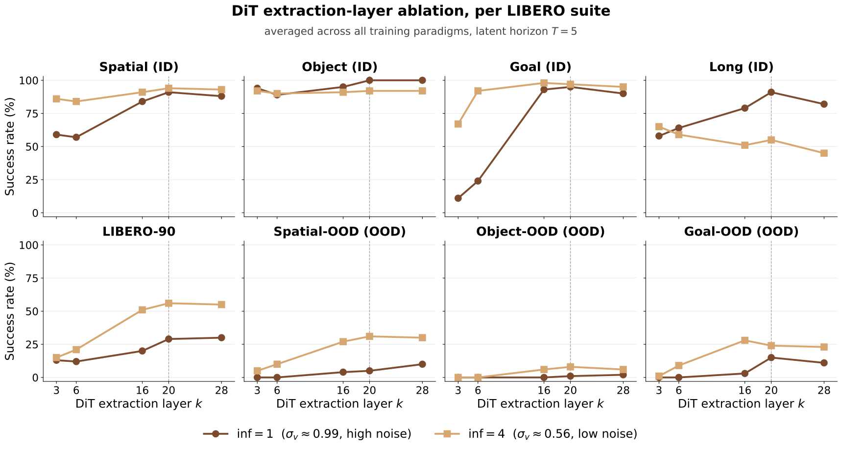
Intermediate video blocks balance geometric detail and semantic structure. Block 20 is the selected overall compromise, supported by success tables and attention visualizations. It is not the maximum in every table cell: at the high-noise setting, block 28 has slightly higher OOD success. The paper’s high-noise descriptions also vary between approximately 0.99 and 0.953.
| Noise level | ID | OOD | ID | OOD | ID | OOD | ID | OOD | ID | OOD |
| inf1 () | ||||||||||
| inf4 () | ||||||||||
C.4 Gemma Layer selection for TR
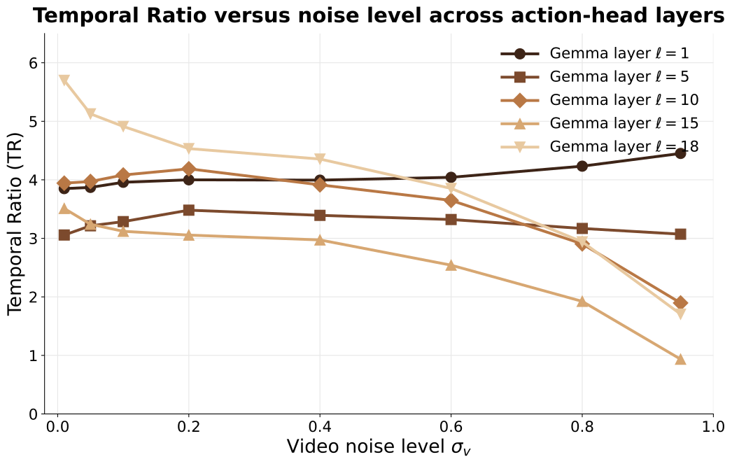
Shallow action-transformer layers show relatively constant TR, whereas layers 15 and 18 vary more with execution and outcome. Layer 15 is used for guidance. With four future frames and one anchor, nearly uniform attention yields TR near four, illustrating why raw TR cannot be interpreted as a per-frame preference or confidence score.
Appendix D Implementation and Hyperparameter Details
D.1 Video Backbone Adaptation
The tables preserve the full optimization settings; the prose highlights choices needed to interpret the experiments.
LoRA adaptation.
LoRA uses rank 32 and matching scale, targeting attention and feed-forward projections throughout all 28 video blocks. It updates roughly 2–6% of backbone parameters with a learning rate of 0.0001.
Full finetuning.
Full finetuning updates the complete backbone. The source gives conflicting learning rates: 0.000001 in the main design-axis description and 0.00001 in Table 8. Neither is silently selected here.
Joint and two-stage training.
Joint training runs 50,000 steps with equal video-loss weight; two-stage training uses 25,000 video-only steps followed by 50,000 action-head steps with frozen, cached video features. Table 8 specifies AdamW, gradient clipping, exponential moving averages, and a total batch size of 128 across 16 GPUs.
| Hyperparameter | LoRA | Full FT |
| Learning rate | ||
| LoRA rank | 32 | – |
| LoRA | – | |
| LoRA targets | all and MLP projections, blocks | – |
| Trainable params | – of B | B () |
| Optimizer | AdamW () | same |
| Weight decay | ||
| Gradient clip (norm) | ||
| Training steps | k joint, k Stage 1 | k joint |
| Batch size | per GPU GPUs | same |
| LR schedule | cosine decay to | same |
| EMA decay | (constant) | |
| Video noise schedule | ||
| Joint loss weight |
D.2 Action Head Training
Action flow matching.
The action head uses flow matching with a biased Beta noise distribution and ten Euler inference steps. Its independent optimization and noise settings are preserved in Table 9.
Action chunking.
Appendices A and D specify 17-action simulation chunks with ten actions executed per replan, while the main setup says 16. The seven-dimensional control vector is padded to 32 internally; action-coordinate descriptions also differ between pose deltas and joint deltas. These inconsistencies need resolution for exact reproduction.
| Hyperparameter | Value |
| Architecture | Gemma expert (App. A.1; layers, M) |
| Action prediction | flow matching (single-step training, -step Euler inference) |
| Action chunk size | steps |
| Action dim | per arm (LIBERO); padded to internal dim |
| Proprioceptive dim | , padded to internal dim |
| Action noise schedule | |
| Learning rate | |
| Training steps (joint and two-stage) | k |
| Optimizer | AdamW () |
| Weight decay | |
| Gradient clip (norm) |
D.3 Feature Extraction
Extraction layer and video noise level.
The default feature source is block 20 at video noise 0.883. The sweep spans fully noisy through nearly denoised features; Table 10 records the tested levels and horizons.
Prediction horizon.
The ordinary policy input represents five latent frames. Plan guidance generates 24 before selecting the first five; this tests longer contextual prediction without enlarging the action-transformer input.
| Parameter | Values |
| Extraction layer | (of DiT blocks) |
| Latent temporal frames | ( video frames) |
| Spatial latent resolution | (from input) |
| Feature dim | |
| Video tokens per latent frame | (after patchify) |
| Video tokens fed to action head | |
| values (inf step ) | |
| Video solver steps | (FlowUniPC, shift ) |
| Action Euler steps |
D.4 Guidance Hyperparameters
Language guidance.
The language branch removes text conditioning in the video model. Its action-velocity difference from the conditional branch is scaled with base weight 0.1.
Plan guidance.
The plan branch uses the extended, truncated video features and base weight 0.3. Its difference from ordinary conditional action velocity supplies the second guidance direction.
TR-adaptive schedule.
Both base weights are multiplied by clip(TR/TR₀ − 1, 0, 2), using layer 15 and an episode-specific initial ratio. The maximum multiplier is two; guidance is inactive at or below the initial ratio and its weights remain fixed within each replan.
Appendix E Real-World Setup and Evaluation Details
E.1 Hardware Description
The physical setup uses two I2RT YAM six-degree-of-freedom arms with grippers, giving 14 controlled joint/gripper values, plus three cameras. Figure 9 shows the platform and evaluation scenes. [18]
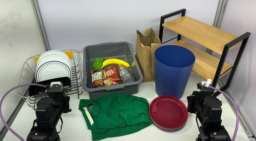
E.2 Bimanual YAM Platform
Observation space.
Three RGB views are resized to 224 × 168 pixels and concatenated horizontally into a 672 × 168 image. Recorded video at 30 frames per second is subsampled to 10; the 17-frame video target includes the current anchor and predicted future observations.
Action space.
The action head predicts 50 steps at 30 Hz and executes the first 30 before replanning, approximately once per second. Both arms and grippers are controlled together.
Latent token count.
The wider camera composite produces 2,310 video tokens across five latent frames, compared with 490 in simulation. The temporal structure remains fixed while spatial token count grows.
E.3 Real-World Training Dataset
Dataset.
The paper’s training set contains 5,600 episodes across 24 tasks, about 9.98 million recorded frames and 3.3 million after subsampling, with 1,036 instruction strings. Twenty-three tasks have 200 episodes each; the relative-placement task has 1,000.
Task families.
The task families are one folding task, two garment tasks, one assembly task, and 20 pick-and-place tasks. Table 12 retains their complete names, descriptions, and episode counts.
Sampling weights.
Training samples tasks uniformly rather than in proportion to their episode counts. Thus the larger relative-placement dataset does not automatically receive five times the task-level sampling weight.
| Skill family | Task | Episodes |
| folding | Fold a pile of t-shirts and stack them | 200 |
| garment manipulation | Remove the shirt from the hanger | 200 |
| Remove the t-shirt from the hanger | 200 | |
| high-precision assembly | Unscrew bottle caps | 200 |
| pick-and-place | Place mixed dishes and glasses into a plastic bin | 200 |
| Place plates into a plastic bin | 200 | |
| Bimanual object handoff | 200 | |
| Load bowls into a tabletop dish rack | 200 | |
| Load cups into a tabletop dish rack | 200 | |
| Load mixed dishes into a tabletop dish rack | 200 | |
| Load plates into a tabletop dish rack | 200 | |
| Place and organize beverages on a shelf | 200 | |
| Place and organize canned foods on a counter | 200 | |
| Place and organize chip bags on a shelf | 200 | |
| Place fake fruits into a fruit bowl | 200 | |
| Place snacks into a paper bag | 200 | |
| Place an object at a specified relative position | 1000 | |
| Take snacks out of a paper bag | 200 | |
| Throw plastic bottles into a bin | 200 | |
| Turn a mug right-side up | 200 | |
| Unload bowls from a tabletop dish rack | 200 | |
| Unload cups from a tabletop dish rack | 200 | |
| Unload mixed dishes from a tabletop dish rack | 200 | |
| Unload plates from a tabletop dish rack | 200 |
E.4 Real-World Compositional Evaluation
Evaluation scenes.
Evaluation introduces scenes with multiple candidate destinations: fruit with a bag and bin; snacks and bottles with a bag and bin; and snacks with a bin and shelf. Training usually supplies a single destination. Some tested bindings are familiar and others recombine known objects and goals.
Task definitions and trials.
The two fruit instructions each receive 15 trials, split across three fruits. The other six instructions receive five each, totaling 60 per policy. Success requires approaching and picking the named object first, then reaching the named receptacle. Table 13 preserves each instruction and count; the paper’s discussion of 50% performance is a task-specific diagnostic, not a universal chance baseline.
| Task | Instruction | Scene | Trials |
| 1 | Throw away the fruits into the bin | 1 | 15 |
| 2 | Place the fruits into the paper bag | 1 | 15 |
| 3 | Place snacks into the paper bag | 2 | 5 |
| 4 | Throw away the snacks into the bin | 2 | 5 |
| 5 | Place plastic bottle into the paper bag | 2 | 5 |
| 6 | Throw away the plastic bottle into the bin | 2 | 5 |
| 7 | Place snacks into the bin | 3 | 5 |
| 8 | Arrange snacks on the shelf | 3 | 5 |
| Total trials per method | 60 | ||
E.5 Real-World Training Hyperparameters and Compute
Optimisation.
Real-world training uses joint video/action optimization, rank-32 LoRA at learning rate 0.0001, and an action-head peak rate of 0.0005 with warmup and cosine decay. The schedule description gives 10,000 steps, whereas the compute paragraph and Table 14 report one million optimizer steps; the source does not reconcile them.
Baselines.
Comparisons include π₀, π₀.₅, and the authors’ Cosmos-Policy implementation. They report matched real-world data and compute, but also unsuccessful Cosmos-Policy training. Its low scores therefore do not isolate architecture quality from implementation or optimization failure. [4] [20] [22]
Compute budget.
Table 14 reports 32 H200 GPUs, effective batch size 512, bfloat16 precision, and one million optimizer steps per method. These are reported training resources, not inference-speed measurements.
E.6 Inference Cost
Guidance trades additional computation for improved compositional success. TR itself reuses attention from the conditional action pass, but both counterfactual branches require extra model work.
Forward-pass cost.
The video-feature computation can increase from one branch to three: conditional, text-free, and extended-plan. Although this section describes action-head cost as unchanged, Algorithm 3 evaluates the action head for active counterfactual branches too, up to three times per integration step. No measured end-to-end latency is provided, so a fixed total slowdown cannot be inferred.