At a glance
The model combines a continuum of agents with multidimensional outcome valuations, finite strategies that share congested resources, and optional hard capacities. Equilibria admit aggregate-flow and outcome-threshold descriptions; welfare-optimal assignments use semi-discrete optimal transport and strategy-level dual potentials. With utility valuation minus latency and convex total resource costs xℓ(x), welfare maximization is convex and a social optimum can be supported by marginal-cost tolls plus capacity multipliers. The results characterize structure and existence under stated assumptions; no convergent numerical solver or empirical mobility deployment is demonstrated.
I Introduction
The paper connects heterogeneous allocation preferences with endogenous congestion, then separates equilibrium and welfare characterizations.
I-A A New Congestion Game Model
Agents can value destinations, charging stations or service outcomes differently while their strategies consume shared resources. A valuation vector records these preferences, and congestion depends on the resulting allocation. This joins multidimensional assignment with network congestion, rather than representing heterogeneity only by one participation cutoff.
I-B Theoretical Contributions
Three results drive the paper. First, used strategies for a given outcome have minimum equal latency at equilibrium, producing one outcome-threshold vector per group. Second, fixing aggregate flows turns optimal type-to-strategy assignment into semi-discrete transport, with finite strategy-indexed dual potentials. Third, separable utility produces a convex planner problem and marginal-cost/capacity pricing under additional regularity. The equilibrium and optimal-transport arguments have different origins; the dual vector is not automatically an implementable congestion price.
I-C An Emerging Application
Advanced air mobility motivates joint destination/route choice with both delays and infrastructure limits. The paper supplies a static model for this setting, not an operational air-traffic mechanism. Its notation uses componentwise vector order, measurable pushforwards and almost-everywhere statements over the continuum population.
II Related Work
The main connections are nonatomic congestion games, continuum matching and semi-discrete transport. The new combination concerns multidimensional outcome values with endogenous congestion.
II-A Nonatomic Congestion Games
Compared with player-specific single-resource games, strategies may use several shared resources and utility need not separate valuation from latency. Elastic-demand routing is recovered through an outside option, while multiple outcomes require a multidimensional partition. Destination-choice preferences need not follow a prescribed parametric random-utility distribution.
II-B Matching Markets
Threshold geometry resembles continuum college matching, but the model is one-sided, with cardinal utilities and congestion externalities. It studies Nash equilibria and welfare optima, rather than stable two-sided matchings. Prior finite matching-with-congestion models do not give the same continuum/network characterization.
II-C Optimal Transport for Nonatomic Games
Other transport approaches analyze Cournot–Nash equilibria or physical movement through congested space. Here optimal transport assigns types to a finite strategy set conditional on its target masses; the outer optimization chooses those masses. It does not transport travelers geometrically between prescribed origin/destination distributions.
III Model
The primitives specify resources, groups, outcomes, strategies, valuation distributions and utilities; the solution objects initially assign a strategy to every type.
III-A Nonatomic Congestion Games with Heterogeneous Valuations
Each group has a finite strategy set partitioned by outcome. Its finite measure describes the total mass of agents at each valuation vector.
III-A 1 Elements
Resources have positive capacities and nonnegative, nondecreasing continuous latency functions. Strategy latency sums the latencies of its resources. The main model uses individual resource capacities; later extensions permit coupled constraints.
III-A 2 Agents, Outcomes, and Strategies
Group i has mass rᵢ, outcomes Dᵢ and strategies 𝒫ᵢ, with each strategy a subset of resources and assigned to exactly one outcome. Strategies are group-indexed/disjoint as labels, even when they share resources. In routing, an outcome is a destination and a strategy is a path to it.
Equation
III-A 3 Flows
Strategy flows are nonnegative masses. Admissibility requires each group’s flows to sum to rᵢ; resource loads sum all strategy flows using that resource. Capacity feasibility adds load≤capacity. Latencies depend on these aggregate loads, not on the identity of individual agents.
Equation
III-A 4 Always-Feasible Strategies
Each group must have a strategy consisting entirely of nonbinding-capacity resources. This guarantees an always-feasible alternative, interpretable as not participating. It is essential to arguments excluding overloaded equilibria in the basic capacity model.
Equation
III-A 5 Valuations
Valuations lie in a compact nonnegative box, with total population measure rᵢ. The measure is a deterministic distribution of types, not uncertainty about an individual’s private draw. Main results assume absolute continuity with respect to Lebesgue measure, so outcome indifference sets are null; arbitrary measures are handled later with splittable type masses.
Equations
III-A 6 Action Profiles
A measurable pure action profile pushes the population measure onto strategy flows. Lemma 1 shows that every admissible flow can be realized: nonatomicity permits partitioning each group’s type space into measurable pieces with the requested masses. Profiles differing only on null sets are equivalent. This realizability statement alone does not establish equilibrium existence.
Equations
III-A 7 Utility Functions
Utility Uᵢ(value,latency) is continuous, strictly increasing in value and strictly decreasing in latency. Soft congestion changes latency continuously; a strategy using an overloaded resource instead receives −∞, or a sufficiently low finite substitute. The always-feasible option makes such a strategy unattractive in the basic model. Separable utility value−latency is a later specialization.
Equation 1
| (1) | ||||
III-A 8 Instances
An instance collects the resource and strategy sets, group masses, latency/capacity data, valuation spaces with their measures, utility functions and outcome partition. These primitives determine both population sorting and congestion.
III-B Relation to Classical Nonatomic Congestion Games
Classical nonatomic congestion games are recovered after allowing strategy-specific resource consumption weights and homogeneous valuation masses with infinite capacities. A homogeneous type is an atom in valuation space but still represents many infinitesimal agents, not one strategic player with positive weight. Thus this reduction uses the later general-measure extension, beyond the main absolute-continuity assumption.
Equations
III-C Nash Equilibria and Social Optima
Nash equilibrium tests individual best responses at unchanged aggregate flow; social optimality maximizes integrated utility over assignments.
III-C 1 Nash Equilibria
Almost every infinitesimal agent must weakly prefer its chosen strategy to every alternative. A unilateral deviation has zero effect on aggregate load, including at a binding capacity. This convention differs materially from equilibrium definitions that permit only positive-mass coalitional deviations.
Equation
III-C 2 Social Optima
Social welfare integrates realized utility over all groups and types. Two assignments with the same flow can have different welfare because they assign different valuations to outcomes. The planner therefore optimizes both the flow and which types realize it.
Equations 2
| (2) |
III-D Problem Formulation
The central question is whether infinitely many individual choices can be represented by finite variables. The answer uses aggregate flows plus outcome thresholds for equilibrium and aggregate flows plus strategy dual potentials for general welfare; separability enables explicit supporting prices.
IV Applications
Routing, shared markets and congestible clubs illustrate the framework’s scope. They are mathematical examples, not empirical validations.
IV-A Routing Games with Heterogeneous Valuations
Routing groups share a source but may choose among several destinations. An outside destination can represent not traveling.
IV-A 1 Model
Strategies are simple paths, utility is destination value minus path latency, and the specialized latency assumptions require differentiability and convex xℓ(x). The marginal-cost function is ℓ(x)+xℓ′(x). Multiple destination values generally have no single ordering; zero-valued outside options or homogeneous types fit through the general-measure extension when they violate full-dimensional absolute continuity.
Equations
IV-A 2 A Two-Destination Example
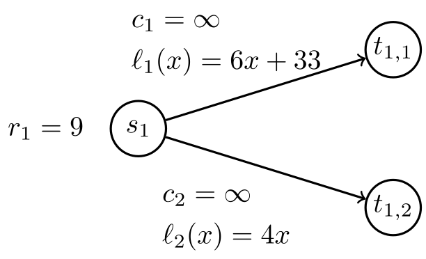
In the two-destination example, type mass is Lebesgue measure on [0,3]², totaling nine. Equilibrium threshold (2,0) assigns flows (0.5,8.5), with latencies (36,34), so choice is determined by v₁−2 versus v₂. The optimum threshold (1,0) gives flows (2,7) and marginal costs (57,56). Destination heterogeneity permits unequal used-route latencies, so merging both destinations into a single classical endpoint loses the essential sorting structure.
Equations
IV-B Market-Sharing Games
An agent serving market j obtains value times its share nⱼ/fⱼ, represented by a nonseparable value/latency utility. The literal ratio is singular at zero and does not meet the model’s assumptions. The paper therefore supplies positive numerator/denominator regularization, restoring continuity and strict monotonicity.
Equations
IV-C Congestible Club Goods
Clubs, coworking spaces or fitness facilities are outcomes with membership-dependent congestion and heterogeneous membership values. Capacities represent membership/physical limits; shared resources across facilities motivate coupled constraints.
V Characterizations of Nash Equilibria and Social Optima
The finite description retains both how much traffic each strategy carries and which valuation types receive each outcome. General welfare additionally needs the assignment among same-outcome strategies.
V-A Characterization of Nash Equilibria
Equilibrium existence and its conditional threshold characterization are distinct results.
V-A 1 Existence and Nonexistence
Without binding capacities, continuous aggregate utilities, measurable preferences and finite strategies satisfy Schmeidler’s nonatomic-game existence conditions. Hard capacities break this continuity and can destroy Nash equilibrium under individual zero-mass deviations. The paper does not assert universal existence in the capacitated model.
Equation
V-A 2 Threshold-Based Characterization
Theorem 1 gives three necessary and sufficient flow conditions: capacity feasibility; each used strategy minimizes latency among strategies to its outcome; and each outcome’s flow equals the measure of types maximizing Uᵢ(vⱼ,τᵢⱼ), where τ is minimum outcome latency. Strict value monotonicity plus absolute continuity makes ties null by fixing all but one valuation coordinate. Conversely, measurable partitions allocate each outcome region among its minimum-latency strategies at the required masses. Thus the thresholds describe sorting while the flow consistency conditions close the congestion feedback.
Equations 3
| (3) |
V-A 3 Computational Approach
These conditions suggest a finite-dimensional fixed-point computation. No particular algorithm’s convergence or runtime is established; that is explicitly future work.
V-B Characterization of Social Optima
Welfare optimization separates into an outer choice of feasible strategy masses and an inner optimal assignment at those masses.
V-B 1 Upper-Level Problem
For fixed flow f, all strategy latencies are fixed. The value Sᵢ(f) maximizes group i’s integrated utility over measurable assignments whose pushforward is fᵢ. The outer problem maximizes the sum of these values subject to flow conservation, nonnegativity and capacities. Lemma 1 makes every candidate admissible flow realizable.
Equations 4–5d
| (4) |
| (5a) | ||||
| s.t. | (5b) | |||
| (5c) | ||||
| (5d) | ||||
V-B 2 Semi-Discrete Optimal Transport
A Kantorovich coupling may split source mass; a Monge map assigns each type deterministically. Lemma 2 uses a nonatomic source, finite targets and bounded continuous reward to equate the transport optimum with a finite dual minimum: integrate the maximum reward minus a target potential, then add potential-weighted target masses. Both extrema are attained, and every optimal dual vector supports some optimal measurable map. The map selection must respect target masses; arbitrary tie-breaking is insufficient.
Equations 6
| (6) | ||||
V-B 3 Lower-Level Problem
Theorem 2 applies that lemma to utility at fixed congestion, with one dual potential per strategy. Optimal assignments select utility-minus-potential maximizers and meet prescribed strategy masses. Same-outcome strategies can tie over positive-measure regions, so their supporting regions need not form a disjoint partition. Translation invariance and a uniform utility bound permit an optimal potential vector in [0,2K]. These are conditional assignment prices, not generally resource-level congestion tolls.
Equations 7–8
| (7) | ||||
| (8) |
V-B 4 Existence and Comparative Statics
Joint continuity and the fixed compact dual box give continuous assignment value and an upper-hemicontinuous nonempty compact optimizer correspondence via Berge’s theorem. Compact feasible flows then yield existence of a social optimum. The max-of-shifted-utilities integrand is submodular in potentials, so the minimizing set is a compact sublattice and hence a complete lattice with extremal selections. This concerns the bounded dual set; it does not prove unique flow or smooth comparative statics.
Equations
V-B 5 Computational Approach
Each fixed-flow assignment dual is convex and finite-dimensional, but the general outer welfare problem can remain nonconvex. Finite-dimensional characterization should not be read as an efficient global numerical algorithm.
VI Inducing Social Optima under Separable Utilities
Now specialize to value−latency, differentiable standard latencies with convex xℓ(x), and the constraint qualifications needed for KKT multipliers. Assignment depends only on destination masses once congestion cost is separated.
Equation
VI-A Social Welfare Optimization Problem
Total congestion cost is ∑ₑfₑℓₑ(fₑ), independent of which types realize a fixed flow. The inner value now maximizes valuations alone and has one dual potential per outcome, not per strategy. Its optimal assignment chooses vⱼ−τᵢⱼ and yields outcome masses equal to threshold-region measures. The symbol Sᵢ is reused here for this valuation-only value; it excludes latency unlike its earlier definition.
Equations 9a–12
| (9a) | ||||||
| s.t. | (9b) | |||||
| (9c) | ||||||
| (9d) | ||||||
| (10) |
| (11) |
| (12) |
VI-B Comparative Statics and Convexity
The valuation-only value is a pointwise minimum of affine flow functions, hence concave. Danskin’s theorem describes its supergradients through optimal outcome potentials, repeated across strategies sharing an outcome. A singleton dual solution gives the stated differentiability result for the paper’s ambient concave extension. Subtracting convex total latency preserves a concave welfare objective over linear constraints, yielding a convex optimization problem. This conclusion requires more than merely nondecreasing latency.
Equations 13
| (13) |
VI-C First-Order Characterization of Social Optima
Theorem 3 combines a compatible optimal assignment potential τ with nonnegative capacity multipliers δ. Nonbinding resources have zero multiplier; every used path maximizes threshold value minus marginal-cost latency minus summed capacity prices. The proof derives these inequalities from KKT stationarity/complementarity and reconstructs the remaining multipliers for sufficiency. Without capacity limits the δ terms vanish, recovering marginal-cost optimality with heterogeneous destination choice.
Equations 14–19
| (14) |
| (15) |
| (16a) | |||||
| (16b) | |||||
| (16c) | |||||
| (16d) | |||||
| (17) |
| (18) | ||||
| (19) |
VI-D Implementation of Social Optima
Fixed resource prices add to perceived latency. The resulting equilibrium flows maximize valuation-assignment value minus the Beckmann integral potential and the linear price bill. Setting perceived latency to ℓ+xℓ′ and prices to optimal capacity multipliers makes a selected social optimum an equilibrium of the unconstrained priced game. Equivalently, charge the congestion externality xℓ′ plus a capacity fee. This is a supporting-price existence result at an optimum, not a proof that every equilibrium under fixed prices is capacity-feasible or that a practical adaptive pricing process converges. Prices can be interpreted as monetary transfers or delays, but the original welfare objective does not separately add fee revenue or waiting costs.
Equations 20–23
| (20) |
| (21a) | ||||||
| s.t. | (21b) | |||||
| (21c) | ||||||
| (22) |
| (23) |
VII Extensions
Two extensions cover coupled aggregate constraints and type distributions with atoms.
VII-A General Constraints
Continuous coupled constraints replace per-resource capacities, with a nonempty feasible-flow set assumed. The equilibrium characterization is restricted explicitly to constraint-feasible equilibria: a lower-bound violation may otherwise persist at an all-outside Nash profile because one infinitesimal entrant cannot change the deficient load. Inner assignment duality is unchanged. Convex differentiable constraints and standard latencies preserve convex welfare optimization; suitable constraint qualification supplies supporting multipliers.
Equation
VII-B General Measures
An arbitrary finite type measure may put positive mass on one valuation vector. Represent actions by measurable kernels that split that type’s mass over strategies; constant probabilities fₚ/rᵢ realize any admissible flow. An atom here is a collection of infinitesimal identical agents, not an atomic strategic player. Positive-mass ties require split assignment rather than almost-everywhere unique outcome choice.
Equations
VIII Conclusion
The paper provides structural and existence results linking multidimensional sorting, congestion and optimal transport. Applications include destination/vertiport allocation and supporting landing fees, under the separable assumptions. Price-of-anarchy bounds, reliable numerical methods and dynamic mechanisms that learn without knowing valuation distributions remain open. There are illustrative examples but no experimental performance claims or deployment evidence.
Acknowledgment
The authors disclose using GPT-6 Astra to help check and revise proofs in Sections V–VII and Appendix A. This is their stated assistance disclosure, not independent proof verification by this edition.
References
The original 51 bibliography entries are retained in the citations view, with linked references from the notes.
Appendix A Proof of Lemma 2
For any optimal dual vector, strong duality forces an optimal coupling onto reward-minus-potential maximizing targets. Disintegration yields measurable target-selection probabilities. Nonatomicity and Lyapunov’s convexity theorem purify this finite-target kernel into a deterministic selection with the same target masses. Integrating the resulting tight dual equality proves that the map is optimal. This mass-preserving purification, rather than arbitrary pointwise argmax selection, is the key exactness step.
Equations
Appendix B Some Single-Destination Examples
Three one-link examples separate classical routing, excessive participation from congestion externalities, and equilibrium nonexistence caused by a hard cap. Table I summarizes the interventions supporting the optima.
B-A First Example: Classical Routing Games
With unit population, ℓ(x)=x, capacity one and uniform values on [2,3], everyone travels. The unique equilibrium also maximizes welfare, giving 3/2, so no price intervention is needed.
B-B Second Example: Heterogeneous Valuations and Marginal-Cost Tolling
With values uniform on [0,1], equilibrium routes the upper half of values, so flow is 1/2. Welfare is maximized at cutoff 2/3 and flow 1/3. Replacing perceived latency x by marginal cost 2x, equivalently adding toll x, implements that optimum.
B-C Third Example: Capacity Constraints and Capacity Fees
Keep values uniform on [2,3] but cap flow at 1/2. Below or at capacity, an excluded infinitesimal agent wants to enter without changing aggregate load; above capacity, travelers prefer the outside option. Thus the stated Nash notion has no equilibrium. The welfare optimum serves the upper-valued half, cutoff 5/2. With W(x)=3x−(3/2)x², the capacity multiplier is W′(1/2)=3/2. Add marginal toll x plus that capacity fee: total perceived cost is 2x+3/2, inducing flow 1/2. At the optimum, monetary charges total two, distinct from total perceived cost 5/2 including physical latency.
Equations
B-D Relationship with Existing Single-Destination Traffic Assignment Models
Equilibrium terminology changes the answer to existence questions. The appendix relates the paper’s individual-deviation Nash notion to established elastic-demand and capacitated traffic-assignment notions.
B-D 1 Routing Games with Elastic Demand
Without capacity constraints and with one real destination plus an outside option, the equilibrium agrees with standard elastic-demand routing. The explicit continuum of heterogeneous values provides the individual-choice basis for its aggregate demand formulation.
B-D 2 Routing Games with Edge Capacity Constraints
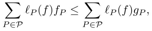
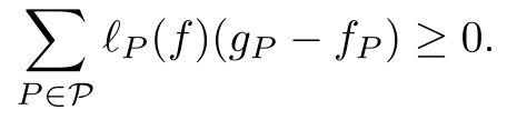
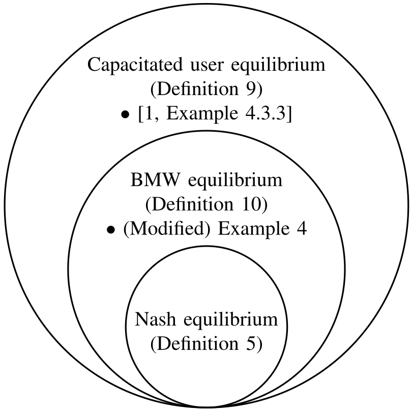
A capacitated user equilibrium excludes profitable deviations by positive-mass sets, allowing binding capacity to block a move. A BMW equilibrium minimizes the Beckmann potential over capacity-feasible flows. Every Nash equilibrium here is BMW, and every BMW equilibrium is a capacitated user equilibrium; both inclusions are strict. Integrating individual latency inequalities gives the BMW variational inequality. Replacing the outside option in the capped example by a constant-cost-one edge gives a BMW half/half flow that is not Nash, since a zero-mass traveler can still switch to the cheaper capped edge. The finite-feasible-set optimization notion has existence even where individual-deviation Nash fails.
Equations 24a–24e
| (24a) | ||||
| s.t. | (24b) | |||
| (24c) | ||||
| (24d) | ||||
| (24e) | ||||

Appendix C Basics of Lattice Theory
Under componentwise order, joins and meets are coordinatewise maxima and minima. Submodular minimizers form a sublattice; a nonempty compact sublattice of Euclidean space is complete. These facts justify extremal bounded dual-potential selections, without requiring the optimizer to be unique.
Equations
Appendix D Details of the Extensions
The extensions preserve the inner transport structure while altering either feasible aggregate flows or the representation of individual type mass.
D-A General Constraints
At an optimal flow, multiply each differentiable aggregate-constraint gradient by its KKT multiplier and sum to obtain a fixed resource price. Add this price to marginal-cost latency to support the optimum in an unconstrained priced game. General constraints can produce negative prices, interpreted as subsidies; coordinatewise nondecreasing constraints give nonnegative prices. The argument assumes a constraint qualification such as relative Slater feasibility.
Equations
D-B General Measures
For general type measures, a destination kernel must put weight only on best-response outcomes and reproduce their target masses. A strategy kernel similarly disintegrates an optimal transport coupling and is supported on dual maximizers. The finite dual characterization remains, but a deterministic map may no longer exist. The original author portraits and biographies following this appendix are retained.
Equations
 |
Pan-Yang Su (Student Member, IEEE) received the B.S. degree in electrical engineering from National Taiwan University, Taipei, Taiwan, in 2022. He is currently pursuing the Ph.D. degree with the Department of Electrical Engineering and Computer Sciences, University of California at Berkeley, Berkeley, CA, USA. His research focuses on applying game theory and mechanism design techniques to study multi-agent systems, with applications in energy and transportation. |
 |
Negar Mehr (Member, IEEE) received the B.S. degree in mechanical engineering from Sharif University of Technology, Tehran, Iran, in 2013, and the Ph.D. degree in mechanical engineering from the University of California, Berkeley, Berkeley, CA, USA, in 2019. From 2019 to 2020, she was a Postdoctoral Scholar in Aeronautics and Astronautics at Stanford University, Stanford, CA, USA. She then served as an Assistant Professor of Aerospace Engineering at the University of Illinois Urbana-Champaign, Urbana, IL, USA, before joining the University of California, Berkeley, in 2024. She is currently an Assistant Professor of Mechanical Engineering and directs the Berkeley Intelligent Control (ICON) Laboratory. Her research interests include control theory, game theory, and machine learning, with an emphasis on safe and intelligent interactions among robots, humans, and other autonomous agents. Dr. Mehr is a recipient of the AFOSR Young Investigator Award, the ONR Young Investigator Award, the NSF CAREER Award, the ASME Rising Star Award, and the IEEE ITSS Best Ph.D. Dissertation Award. |
 |
Shankar Sastry (Life Fellow, IEEE) is a Professor of EECS, Bioengineering and Mechanical Engineering and the Siebel Professor of Computer Science and Engineering at the University of California Berkeley. He was the Dean of Engineering from 2007-18. He is currently the faculty Director of the Technology Competitiveness and Industrial Policy, a center which conducts studies on policy need to enhance US competitiveness and the FHL Vive Center for Enhanced Reality for exploring the boundaries between augmented reality and real scenes with applications to autonomy, performance arts, and education. He is the honorary chancellor of a new technical university in Chandigarh, India called Plaksha University. He is deeply committed to harnessing the power of technology to lift people out of poverty through his directorship of the Blum Center for Developing Economies 2007-22. He has coauthored about 750 technical papers. He has co-authored or co-edited 10 books, including Adaptive Control: Stability, Convergence and Robustness (with M. Bodson, Prentice Hall, 1989) and A Mathematical Introduction to Robotic Manipulation (with R. Murray and Z. Li, CRC Press, 1994), Nonlinear Systems: Analysis, Stability and Control (Springer-Verlag, 1999), and An Invitation to 3D Vision: From Images to Models (Springer Verlag, 2003) (with Y. Ma. S. Soatto, and J. Kosecka). and Generalized Principal Component Analysis (Springer Verlag, 2016 with R. Vidal and Y. Ma). Dr. Sastry was elected to the National Academy of Engineering in 2001 the American Academy of Arts and Sciences in 2004. He received the President of India Gold Medal in 1977, the NSF Presidential Young Investigator Award in 1985. He got the Eckman Award of the American Automatic Control Council in 1990, the Ragazzini Award for Distinguished Accomplishments in teaching in 2005 and the Rufus Oldenburger Career Award of ASME in 2021. He has received honorary doctorates from KTH, the Royal Institute of Technology, Stockholm, a Ph.D. honoris causa from the University of Waterloo, Canada, and a Laurea Dottorato honoris causa from Politecnico di Torino, and the Berkeley Citation. He has supervised more than 75 doctoral students to completion and over 50 Masters of Science Students and is very proud of the leadership positions that they hold in academia and industry. |