At a glance
VLA-Corrector monitors a robot while it executes a predicted action chunk. A separately trained visual-latent dynamics model detects persistent drift, discards pending actions, and guides the next policy query toward recovery. The task-fine-tuned VLA backbone stays frozen. Simulation and robot experiments report better success per policy call, although gradient guidance increases inference time.
1 Introduction
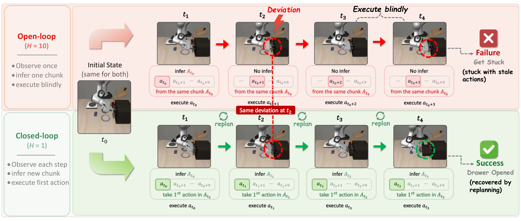
Action chunks amortize expensive policy inference but leave the robot executing old commands while the scene changes. Short fixed horizons restore feedback at the cost of more policy calls. VLA-Corrector instead adapts the executed horizon: it retains a chunk while visual evolution looks consistent, interrupts sustained deviations, and corrects the next replan. The external monitor needs demonstration-based training; freezing the backbone does not make the whole method training-free.
2 Preliminaries
The visual encoder supplies a latent observation to a language-conditioned policy. Each query generates C actions, of which the controller normally executes H before replanning. The corrective module operates during that execution window. It uses predicted versus observed changes in latent features as a consistency signal; this signal is not a ground-truth failure label or a safety certificate.
Equation 1
| (1) |
3 VLA-Corrector: A Lightweight Corrective Inference Framework
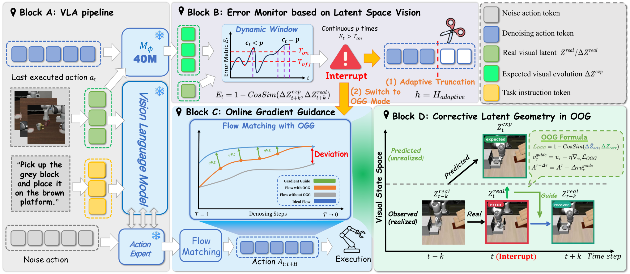
The framework combines an external dynamics predictor, an online deviation monitor, event-triggered truncation, and gradient guidance for recovery. The project repository supplies the implementation.
3.1 Training the External Latent Dynamics Corrector
After task fine-tuning, the VLA encoder and policy are frozen. A residual MLP learns the short-horizon change in visual features from the current latent and executed action. The main formulation combines residual-magnitude error with cosine-direction error. Appendix C describes a cosine-based loss for its deployed correctors; these reported training configurations should be distinguished.
Equations 2–4
| (2) |
| (3) |
| (4) |
3.2 Latent Visual Dynamics for Online Anomaly Detection
The monitor compares the direction of the predicted latent residual with the direction actually observed k steps later. One minus their cosine similarity becomes the inconsistency score. The model learns local demonstrated dynamics rather than reconstructing future images or modeling the entire environment.
Equation 5
| (5) |
3.3 Event-Triggered Truncation under Robust Online Monitoring
A rolling median and MAD set separate activation and deactivation thresholds. Sustained high scores trigger an interrupt, clear the remaining action queue, and mark the next query for correction. Hysteresis, a persistence counter, and cooldown suppress repeated interventions. Their delays and the prediction interval still limit response speed.
Equations 6–7
| (6) |
| (7) |
3.4 Online Gradient Guidance for Corrective Inference
OGG differentiates through the corrector during flow-based action generation, using the flow-matching framework. [26] It estimates a clean action sequence from the current flow state, predicts the latent effect of its first action, and guides that effect toward an expected continuation corrected for the observed deviation. Only the query immediately following an interrupt receives this guidance; later queries return to ordinary inference unless another interrupt occurs.
Equations 8–11
| (8) |
| (9) |
| (10) |
| (11) |
| Backbone | Method | Easy | Medium | Hard | Very Hard | Avg. |
| Baseline | 70.5 | 45.0 | 38.3 | 41.0 | 48.70 | |
| + VLA-Corrector | 83.2 | 61.7 | 47.5 | 65.0 | 64.35 | |
| SmolVLA | Baseline | 81.3 | 53.6 | 51.7 | 61.0 | 61.90 |
| + VLA-Corrector | 83.4 | 56.0 | 64.2 | 63.0 | 66.65 | |
| X-VLA | Baseline | 72.5 | 46.4 | 48.3 | 55.0 | 55.55 |
| + VLA-Corrector | 74.4 | 50.0 | 50.0 | 64.0 | 59.60 |
| Model | Object | Spatial | Goal | Long | Avg. |
| (Full Fine-tuned) | 99.4 | 98.2 | 97.8 | 92.4 | 96.95 |
| (Few-shot Fine-tuned) | 97.8 | 95.4 | 96.2 | 86.6 | 94.00 |
| (Few-shot) + VLA-Corrector | 99.8 | 100.0 | 98.0 | 93.4 | 97.80 |
4 Experiments
Experiments use MetaWorld and LIBERO, compare π0.5, SmolVLA, and X-VLA, and test a physical PiPER arm. Success, policy-query counts, recovery, and inference time measure different aspects of performance. The π0.5 backbone and LIBERO benchmark are described in [15] and [27].
4.1 Main Results
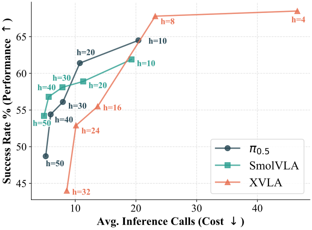
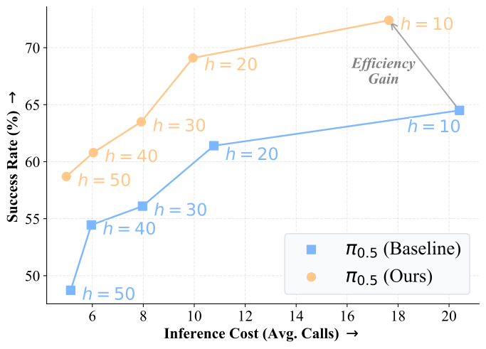
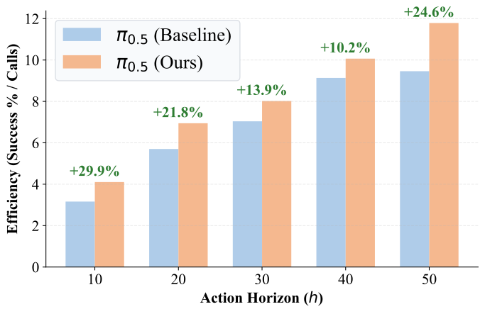
Table 1 reports average MetaWorld gains of 15.65 percentage points for π0.5 (48.70% to 64.35%), 4.75 for SmolVLA, and 4.05 for X-VLA. The separate horizon sweep in Table 4 reports π0.5 at H=50 improving from 48.7% to 58.7%, with calls falling from 5.15 to 4.98. For SmolVLA at H=10, success rises from 61.9% to 73.0% while calls fall from 19.27 to 15.64. The tables report different evaluation settings and should not be combined into one result.
On LIBERO, the few-shot baseline rises from 94.0% to 97.8%, compared with 96.95% for the fully fine-tuned baseline. The corrector also trains on demonstrations. More corrector data helps, with diminishing returns around 60–80% of the post-holdout training pool.
| Method / Ratio | Easy | Medium | Hard | Very Hard | Avg. |
| Baseline | 70.54 | 45.00 | 38.33 | 41.00 | 48.72 |
| VLA-Corrector () | 71.07 | 49.55 | 36.67 | 36.00 | 48.32 |
| VLA-Corrector () | 70.36 | 45.91 | 38.33 | 42.00 | 49.15 |
| VLA-Corrector () | 70.89 | 52.73 | 39.17 | 46.00 | 52.20 |
| VLA-Corrector () | 71.07 | 53.64 | 38.33 | 46.00 | 52.26 |
| VLA-Corrector () | 73.21 | 55.91 | 44.17 | 44.00 | 54.32 |
| Model | Horizon | Baseline | Ours (LVM+OGG) | Improvements | ||||
| Succ (%) | Calls | Succ (%) | Calls | Succ (%) | Calls | Eff. Gain (%) | ||
| 10 | 64.50 | 20.41 | 72.40 | 17.64 | +29.9% | |||
| 20 | 61.40 | 10.77 | 69.10 | 9.95 | +21.8% | |||
| 30 | 56.10 | 7.97 | 63.50 | 7.92 | +13.9% | |||
| 40 | 54.45 | 5.96 | 60.80 | 6.04 | +10.2% | |||
| 50 | 48.72 | 5.15 | 58.70 | 4.98 | +24.6% | |||
| SmolVLA | 10 | 61.90 | 19.27 | 73.00 | 15.64 | +45.3% | ||
| 20 | 58.90 | 11.32 | 68.90 | 9.50 | +39.4% | |||
| 30 | 58.10 | 7.90 | 65.20 | 7.60 | +16.6% | |||
| 40 | 56.80 | 5.64 | 67.20 | 5.13 | +30.0% | |||
| 50 | 54.20 | 4.86 | 62.90 | 4.68 | +20.6% | |||
| X-VLA | 4 | 68.50 | 46.58 | 72.00 | 35.20 | +39.1% | ||
| 8 | 67.80 | 23.18 | 72.10 | 19.48 | +26.5% | |||
| 16 | 55.50 | 13.71 | 60.90 | 13.92 | +8.1% | |||
| 24 | 52.90 | 10.13 | 59.20 | 9.92 | +14.3% | |||
| 32 | 44.00 | 8.61 | 54.40 | 8.34 | +27.6% | |||
- •
Succ: absolute success-rate improvement. Calls: absolute change in policy calls per episode. Eff. Gain: relative improvement in success-per-call over the baseline.
4.2 Mechanism Analysis
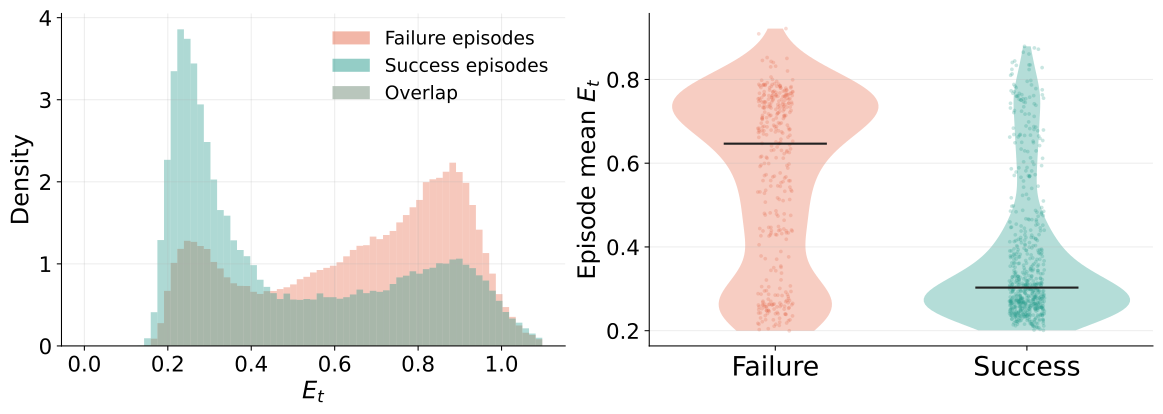
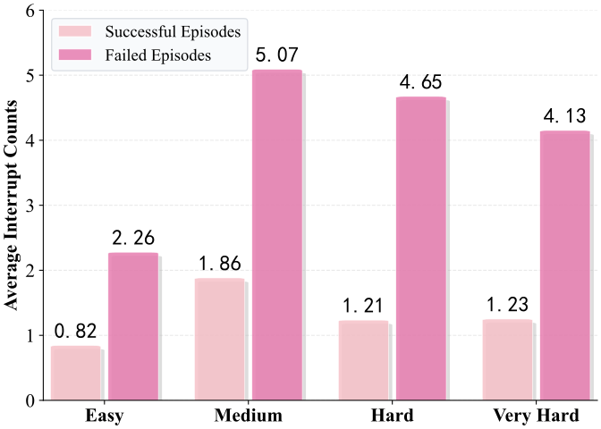
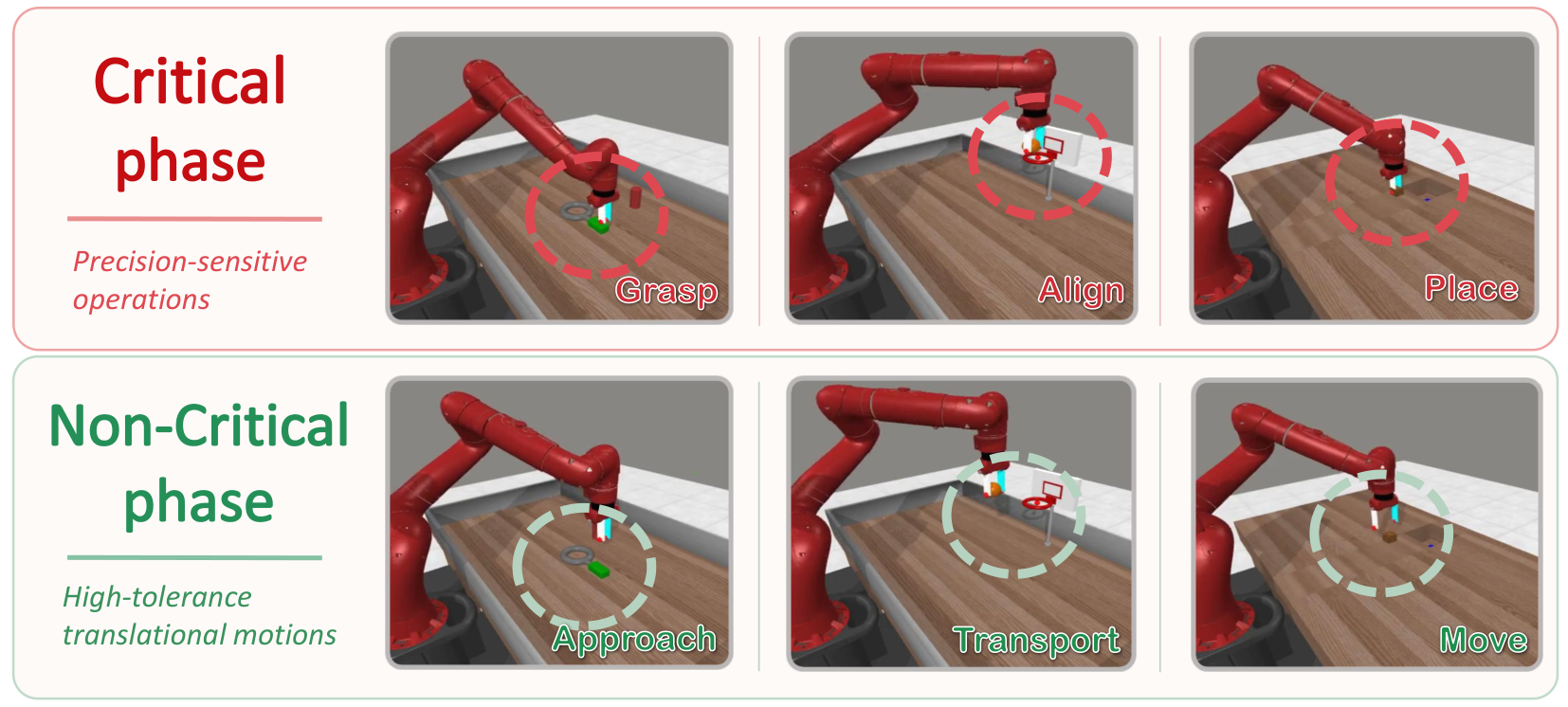
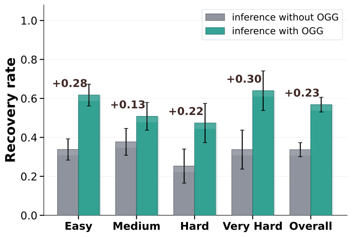
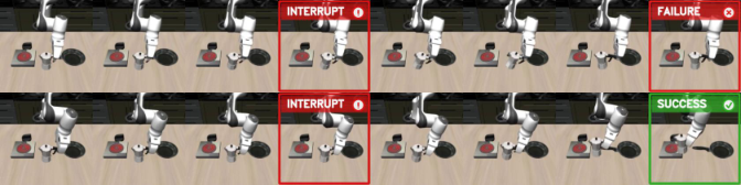
Failed episodes have a heavier high-inconsistency tail. Manual phase labels place 83.7% of truncations in precision-sensitive phases and 16.3% in tolerant phases; this association does not itself prove causality. After matched interruptions, OGG improves the reported recovery rate by an average 0.23. Recovery here means the score drops below the deactivation threshold within ten steps, rather than necessarily completing the task. A controlled grasping example illustrates eventual task recovery.
Truncation Distribution
by Task Phase
Phase
Rate
Critical
83.7%
Non-critical
16.3%
5.1 more truncations occur in critical phases than in non-critical phases.
4.3 Real-World Evaluation
Nine tasks on a six-degree-of-freedom PiPER arm cover pick-and-place, precise alignment, and disturbance recovery. Each method receives 20 trials per task with the same task-fine-tuned π0.5 backbone. Average success increases from 55.6% to 73.3%, with the largest gain in disturbance recovery. Table 5 gives binomial confidence intervals; the appendix reports individual tasks and a different across-task variability statistic.
| Method | Pick-place | Alignment | Disturbance | Avg. |
| Baseline | 70.0 11.6 | 56.7 12.5 | 40.0 12.4 | 55.6 7.3 |
| + VLA-Corrector | 78.3 10.4 | 73.3 11.2 | 68.3 11.8 | 73.3 6.5 |
4.4 Ablation Studies
Truncation alone raises the component-ablation average from 48.70% to 60.35%; adding OGG yields 64.35%. An external detector also outperforms a jointly fine-tuned auxiliary detector, 64.35% versus 49.55%, under the same guidance setting. The proposed explanation—avoiding disruption to backbone representations—is a hypothesis. Moderate guidance and a roughly 40-million-parameter monitor work best in the reported sweeps.
| Variant | Easy | Medium | Hard | Very Hard | Avg. |
| Baseline (Open-loop) | 70.5 | 45.0 | 38.3 | 41.0 | 48.70 |
| + Truncation Only | 81.8 | 53.6 | 50.0 | 56.0 | 60.35 |
| + Truncation + OGG | 83.2 | 61.7 | 47.5 | 65.0 | 64.35 |
5 Conclusion
Monitoring and targeted replanning improve the tested action-chunked policies while keeping their backbone weights fixed during correction. Benefits depend on suitable demonstrations, informative visual features, recoverable disturbances, and actions the backbone can represent. Higher success per query does not imply lower total computation.
Appendix A Related Work
The related work connects generative robot policies, action-horizon selection, and recovery from distribution shift.
A.1 Generative VLA Models
Vision-language-action models combine broad visual and language representations with robot action generation. Diffusion and flow models express complex action distributions but make frequent closed-loop queries costly, motivating a small external monitoring module.
A.2 Action Chunk and Horizon Trade-off
Chunking reduces policy-call frequency and supports temporal coherence, while a fixed long horizon delays reactions. Prior work changes chunking or query schedules; this paper combines an event-triggered horizon with guidance specifically for the following recovery query.
A.3 Failure Recovery in Visuomotor Policies
Recovery approaches expand training data through intervention, learn separate recovery policies, or use search and distribution constraints. VLA-Corrector trains a local latent predictor and guides the existing policy. It still relies on learned dynamics and the frozen policy’s available behaviors.
Appendix B Method Details
The appendix specifies the monitoring state machine and runtime parameters.
B.1 Details of Event-Triggered Truncation
Equation (12) increments the persistence counter above the activation threshold, resets it below the lower threshold, and holds it between thresholds. Reaching the patience value truncates the queue. The surrounding prose describes consecutive high-score steps, but the displayed rule permits intervening scores between thresholds; the original equation is retained to expose that distinction.
Equations 12–13
| (12) |
| (13) |
B.2 LVM and OGG Runtime Parameters
The reported defaults are a 15-score window, MAD multipliers of 3 and 2, patience of five, five safe steps for reset, and a ten-step interrupt cooldown. Guidance strength is 1. OGG applies to a single post-interrupt replan, after which normal inference resumes.
Appendix C Training and Implementation Details
Training and evaluation details distinguish backbone fine-tuning, external corrector training, and online inference.
C.1 Benchmarks and Evaluation Protocol
MetaWorld results average tasks within four difficulty groups, generally with 20 episodes per task. The appendix specifies 10% validation and 10% test episodes before subsampling the remaining training pool, with three split seeds for the data-scaling analysis. The main text calls the held-out 20% validation; both descriptions leave an 80% training pool, but their holdout labels differ.
C.2 External Corrector Architecture
An action embedding is concatenated with the current visual latent and passed through four residual hidden layers of width 2048. Depending on feature and action dimensions, the predictor has approximately 38–42 million parameters. It predicts a feature residual rather than an absolute future feature vector.
C.3 Corrector Training
The corrector uses frozen demonstration features, AdamW, learning rate 0.0003, weight decay 0.0001, cosine scheduling to 1% of the initial rate, and up to 30 epochs with early-stopping patience five. Ratio sweeps use training batches of 128 and evaluation batches of 256; deployed h1-k10 correctors use batches of 512 and a cosine-based loss. The retained equation defines optimization-step counts.
Equation
C.4 Compute Resources
Simulation jobs use a server with eight A100 GPUs, each with 40 GB memory. Monitoring adds an external forward pass; recovery queries additionally backpropagate guidance. Being smaller than a VLA backbone does not eliminate that inference overhead.
Appendix D Additional Experimental Results
Additional results study guidance strength, monitor capacity, domain transfer, and wall-clock cost.
D.1 Ablation Sensitivity
Guidance strength 1 gives the best average in the sweep; stronger guidance harms some difficult tasks. Increasing monitor size from 10 to 40 million parameters improves performance, while 160 million brings little further average gain.
| Guidance Strength | Easy | Medium | Hard | Very Hard | Avg. |
| 82.7 | 56.8 | 45.2 | 66.0 | 62.68 | |
| (default) | 83.2 | 61.7 | 47.5 | 65.0 | 64.35 |
| 82.5 | 56.8 | 38.3 | 65.0 | 60.65 | |
| 80.9 | 55.0 | 36.7 | 63.0 | 58.90 |
D.2 Cross-Domain Corrector Generalization
A LIBERO-trained corrector improves the MetaWorld baseline from 48.7% to 51.8%, while a MetaWorld-trained corrector reaches 58.7% in this comparison. This shows limited cross-domain transfer and a substantial benefit from domain-matched demonstrations.
| Method | Easy | Medium | Hard | Very Hard | Avg. |
| Baseline | 70.5 | 45.0 | 38.3 | 41.0 | 48.7 |
| + LIBERO-trained Corrector | 70.9 | 50.5 | 40.7 | 45.0 | 51.8 |
| + MetaWorld-trained Corrector | 74.1 | 53.8 | 52.9 | 54.0 | 58.7 |
D.3 Inference-Time Overhead
Enabling OGG increases total measured inference time to 1.62–1.68 times that of the same pipeline without guidance. The reported mean cost per executed step rises from 12.32 to 20.25 milliseconds; a guided query takes 588.52 milliseconds versus 278.01 for a standard query. Guidance is intermittent, but the measured total overhead remains material. Policy-call efficiency and wall-clock efficiency must therefore be assessed separately.
| Backbone | Episodes | Steps / Ep. | Calls / Ep. | w/o OGG s / Ep. | w/ OGG s / Ep. | Overhead |
| 1000 | 163.77 | 6.22 | 2.49 | 4.03 | 1.62 | |
| SmolVLA | 1000 | 158.75 | 5.67 | 2.13 | 3.51 | 1.65 |
| X-VLA | 1000 | 177.92 | 10.30 | 1.54 | 2.59 | 1.68 |
| Overall | 3000 | 166.81 | 7.39 | 2.06 | 3.38 | 1.64 |
| Backbone | w/o OGG ms / Step | w/ OGG ms / Step | Extra ms / Step | Relative Overhead |
| 15.23 | 24.62 | +9.39 | 1.62 | |
| SmolVLA | 13.44 | 22.14 | +8.70 | 1.65 |
| X-VLA | 8.66 | 14.55 | +5.89 | 1.68 |
| Overall | 12.32 | 20.25 | +7.93 | 1.64 |
| Backbone | Tasks | Episodes / Task | w/o OGG s / Task | w/ OGG s / Task | OGG Events / Task |
| 50 | 20 | 49.87 | 80.63 | 71.28 | |
| SmolVLA | 50 | 20 | 42.66 | 70.29 | 62.24 |
| X-VLA | 50 | 20 | 30.81 | 51.76 | 119.76 |
Appendix E Real-World Details
The physical experiments document task definitions, trial conditions, observed failures, and example recovery sequences.
E.1 Robot Platform and Task Suite
Both methods use the same camera observations, instructions, action horizon, and task-fine-tuned backbone. Success requires completing the task without a human reset after execution starts. The nine tasks progress from ordinary placements to precise alignment and once-per-trial disturbances.
| Group | Task | Description |
| Pick-and-place | Cube-to-region | Pick up a cube and place it inside a marked target region. |
| Cube-to-drawer-top | Pick up a cube and place it on top of a small drawer platform. | |
| Object-to-container | Pick up a cube and place it into a specific bowl. | |
| Alignment | Corner placement | Place a cube precisely at the upper-left corner of the drawer top. |
| Square-hole insertion | Align and insert a small cube into a square hole or slot. | |
| Edge alignment | Align an object with a narrow marked edge or target strip. | |
| Disturbance recovery | Moving-object grasp | Move the target object when the gripper is about to grasp it. |
| Moving-placement target | Move the placement region after the object is grasped. | |
| Moving-insertion target | Move the square hole or alignment target before insertion. |
E.2 Per-Task Real-World Results
Per-task results show modest gains for ordinary pick-and-place and larger gains for alignment and shifted targets. Table 15 summarizes group and overall variation as standard deviation across tasks; these values differ in meaning from Table 5’s binomial confidence intervals.
| Group | Task | Baseline | + VLA-Corrector |
| Pick-and-place | Cube-to-region | 75.0 | 85.0 |
| Cube-to-drawer-top | 70.0 | 80.0 | |
| Object-to-container | 65.0 | 70.0 | |
| Group Avg. | 70.0 5.0 | 78.3 7.6 | |
| Alignment | Corner placement | 60.0 | 75.0 |
| Square-hole insertion | 50.0 | 70.0 | |
| Edge alignment | 60.0 | 75.0 | |
| Group Avg. | 56.7 5.8 | 73.3 2.9 | |
| Disturbance recovery | Moving-object grasp | 45.0 | 75.0 |
| Moving-placement target | 40.0 | 70.0 | |
| Moving-insertion target | 35.0 | 60.0 | |
| Group Avg. | 40.0 5.0 | 68.3 7.6 | |
| Overall | Avg. across 9 tasks | 55.6 13.8 | 73.3 7.1 |
E.3 Real-World Protocol and Task Details
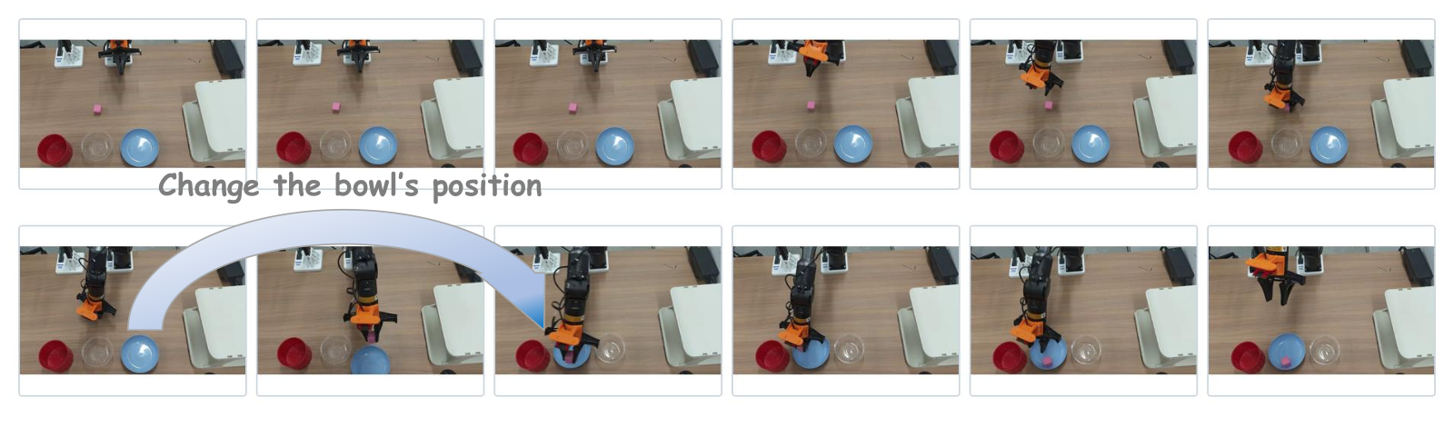
Each task supplies 10–30 teleoperated demonstrations for backbone fine-tuning. Initial poses vary within a small feasible region. Placement tasks use a marked area, drawer platform, or bowl; alignment tasks use a corner, square opening, or narrow edge. Disturbances move an object before grasping or a target before placement/insertion, once per trial, within view and a recoverable range. Both methods use the same phase-based disturbance rules.
E.4 Observed Real-World Failure Modes
Failures remain when a target becomes unreachable, a grasp or timing leaves too little room to recover, contact geometry or friction defeats visual correction, or occlusion and poor contrast obscure the scene. Without force feedback, visual consistency cannot resolve all contact failures. Guidance cannot create recovery behaviors absent from the backbone and supplies no formal collision-avoidance guarantee.
E.5 Real-World Demonstration Examples
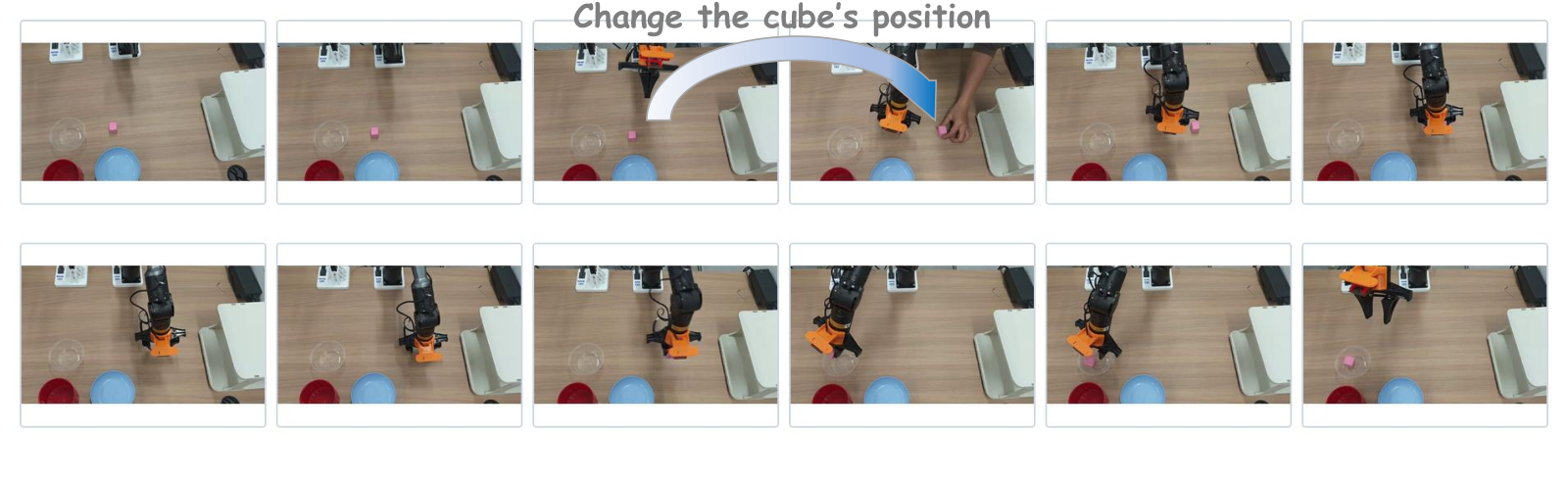
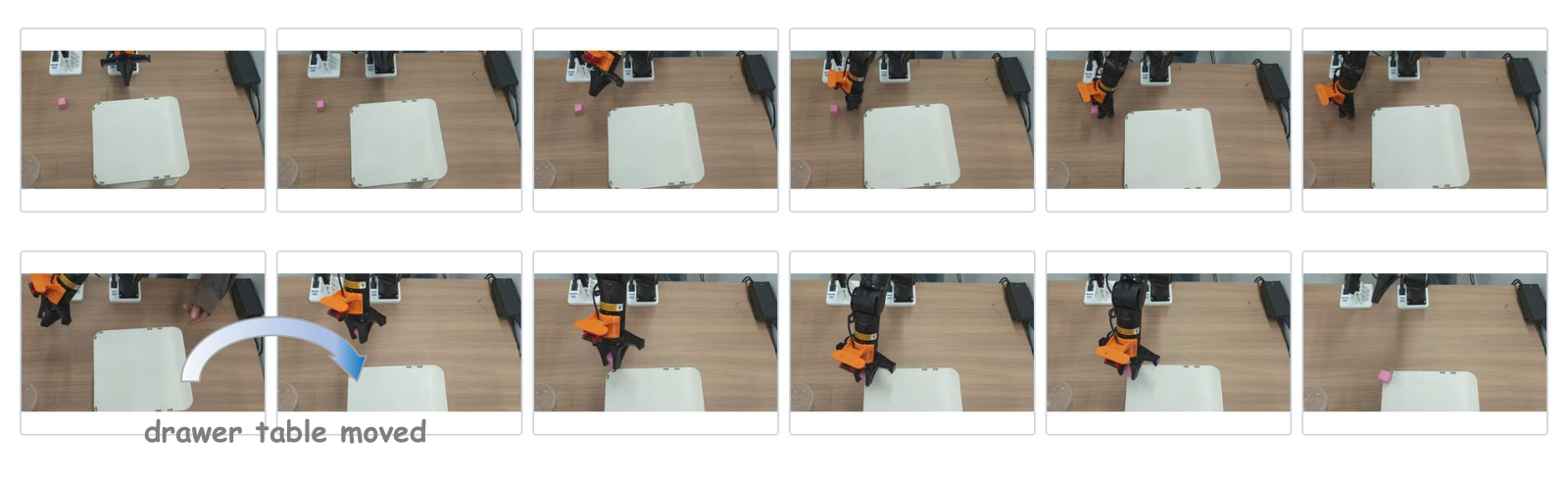
The retained sequences show recovery after a cube, a bowl, or a drawer target is moved during execution. These examples illustrate the mechanism; the trial tables provide the quantitative evidence.