At a glance
This edition follows the complete twenty-nine-page v1, including all twelve numbered figures, six tables, nine equations and supplementary city-scale panels. The task is offline reconstruction of lane centerlines and their directed relations from aerial imagery. A learned geometric prior improves the tested metrics but does not guarantee that an occluded or ambiguous road is reconstructed correctly.
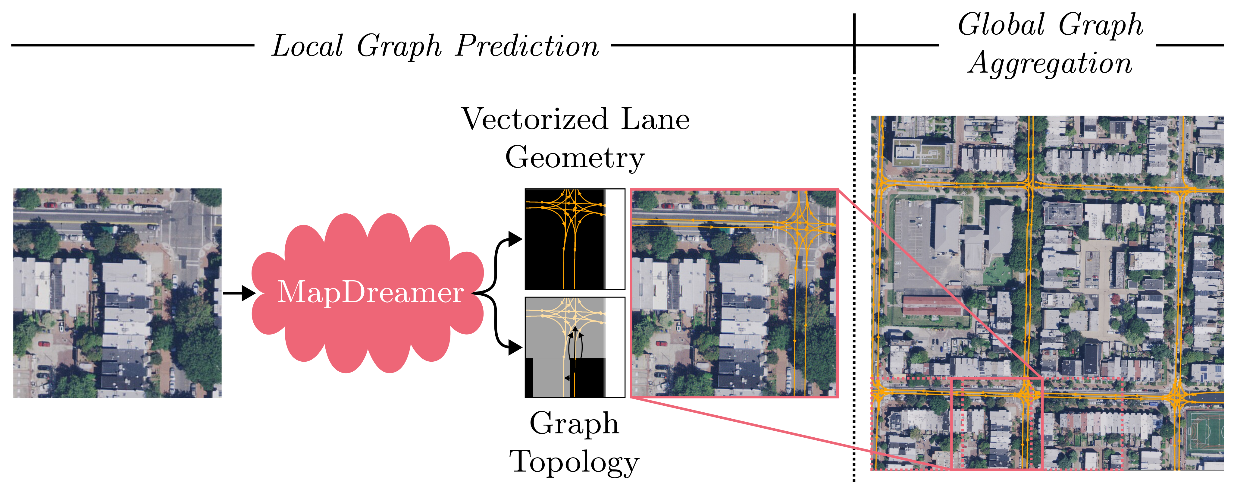
MapDreamer encodes vector lane graphs with a variational autoencoder, then trains an aerial-image-conditioned diffusion transformer in that latent space. A count predictor allocates lane tokens; five spare ghost tokens provide capacity to recover underestimated counts, while an existence head removes unused tokens. Boundary tokens connect sliding-window predictions into larger maps.
On UrbanLaneGraph-derived data, local strict geometry F1 rises from BGFormer’s 0.458 to 0.640 and topology F1 from 0.345 to 0.562. Global results also improve on the reported averages, with qualifications: two Pittsburgh tiles are excluded, LaneGNN uses ground-truth initial poses, and one main-table topology value conflicts with the appendix.
1 Introduction
Aerial views cover large areas, but lane markings, occlusions and intersection structure make directed lane connectivity harder than finding road surfaces. Raster segmentation can lose connections during graph recovery. MapDreamer instead predicts vector centerlines and adjacency jointly, using a learned latent prior and image conditioning to balance plausibility with scene evidence.
Local tiles alone cannot establish consistent large-area connectivity. Neighbor-boundary conditioning carries intersection positions and directions into later tiles; this improves continuity in tested scenes but can also propagate an early wrong interpretation.
Contributions.
The contributions are an aerial-conditioned lane-graph latent diffusion model, count prediction combined with ghost-lane capacity, and boundary-conditioned sliding-window aggregation. Evaluation includes directed geometry, junction-focused connectivity and raster overlap, plus ablations and complete global-map examples.
2 Related Work
2.1 Road Graph Extraction from Aerial Imagery
Road-graph extraction ranges from segmentation and tracing to learned graph representations. RoadTracer grows graphs incrementally; Sat2Graph supervises graph structure through tensor encodings. Transformer and segmentation-foundation-model successors reduce some handcrafted recovery, but road-level networks do not supply all lane-level directions and relations.
2.2 Lane-Level Graph Generation from Aerial Imagery
LaneExtraction combines lane segmentation, direction and intersection processing. LaneGNN/UrbanLaneGraph emphasize directed successor graphs and aggregation from oriented crops. BGFormer represents drivable lanes as Bézier graphs. These are the closest task-level comparisons, though their inference interfaces differ.
2.3 Online Map Generation Using Map Priors
Vehicle-centered map builders infer vector elements from onboard imagery and BEV features; temporal models and map priors add context. Mask2Map, SatForHDMap and SMART address complementary segmentation, satellite fusion and topology problems. MapDreamer instead receives overhead tiles and explicitly predicts directed lane relations for offline reconstruction.
2.4 Diffusion Models for Maps
MapDiffusion denoises online polyline queries, LaneDiffusion injects lane priors into BEV features, and other conditional diffusion work generates raster road networks. MapDreamer denoises graph latents and directly decodes vector geometry plus adjacency. Its evaluation measures reconstruction; it does not calibrate sample uncertainty merely because the generator is stochastic.
Vectorized Generative Simulation.
Scenario Dreamer supplies the vectorized latent-diffusion precedent for synthetic driving environments. MapDreamer adapts that representation to image-conditioned reconstruction of a particular observed scene.
3 MapDreamer
The architecture retains the two-stage graph-autoencoder/diffusion design while replacing free scene synthesis with dense aerial conditioning, an inferred lane budget and neighboring boundary context.
3.1 Scenario Dreamer
Scenario Dreamer first autoencodes lane graphs and agent boxes, then learns diffusion over their latents for scenario generation. MapDreamer uses the lane-graph component rather than claiming to reproduce the predecessor’s full traffic-agent simulation.
3.2 MapDreamer Overview
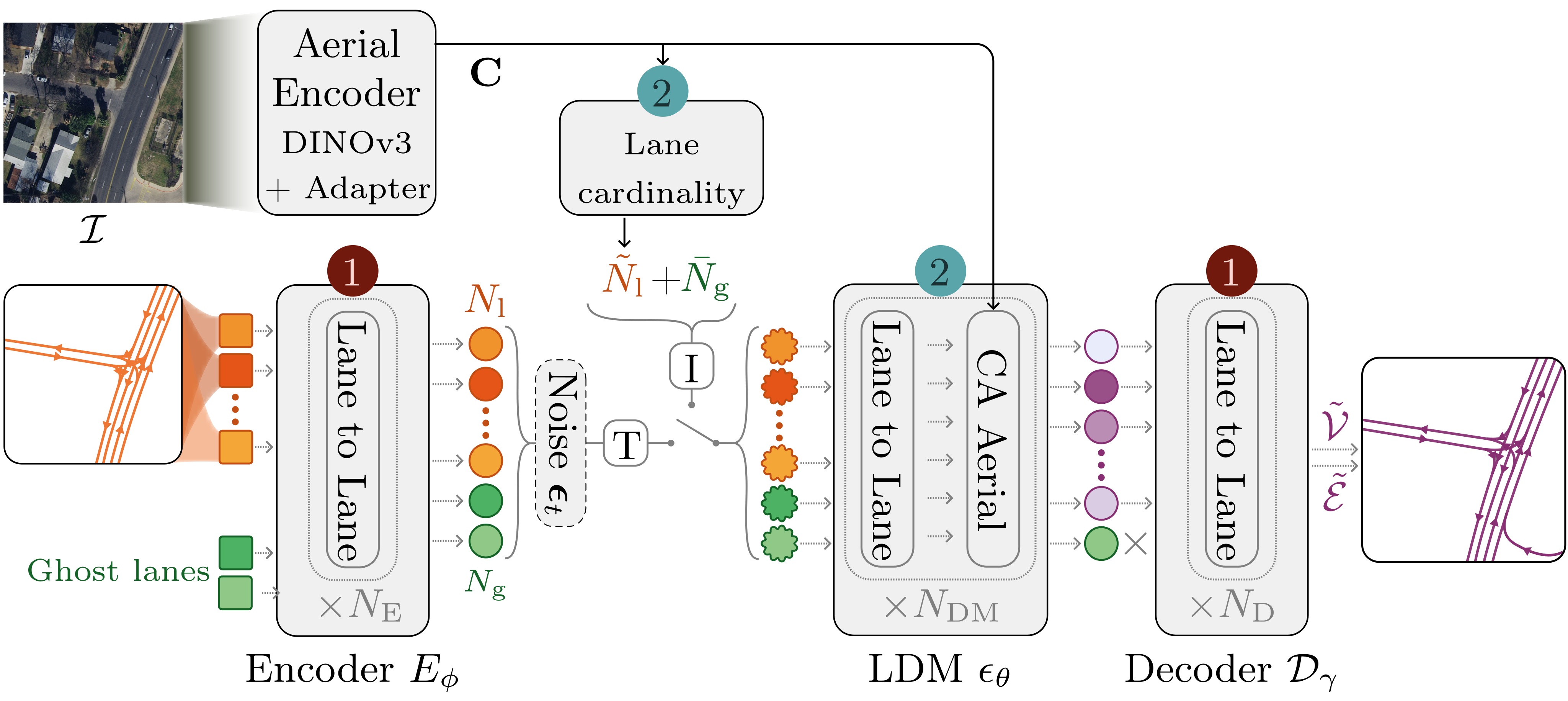
Stage one trains the graph encoder and decoder. Stage two freezes both and trains the denoiser with aerial/count conditioning. At inference, predicted lane count plus spare tokens sets the budget; denoising and existence filtering produce the latents decoded into lane geometry and relations.
3.3 Scene Representation
A 512×512 tile covers 76.8×76.8 metres. Each lane segment is a twenty-point two-dimensional centerline; pairwise successor, predecessor, left and right relations form four adjacency channels. Preprocessing merges degree-two connections so segment boundaries concentrate at splits, merges and genuine or cropped terminations. Fixed dimensionality is per lane latent, while the number of lane tokens varies by tile.
3.4 Model Architecture
Dense frozen DINOv3 features condition every denoising step. A counting module avoids allocating the same large query budget to both sparse roads and busy junctions. Training appends zero to eight ghost targets; inference appends five to the estimated count, chosen against count MAE 3.34.
The buffer permits limited count correction and reduces duplicate hypotheses. It is a finite capacity mechanism: an underestimate beyond the spare budget cannot be repaired by creating unlimited new tokens, and the decoder’s learned prior is not an exact graph-validity constraint.
3.5 VAE
The VAE compresses lane geometry and pairwise relations into a continuous representation. Its frozen decoder supplies a learned structural prior during diffusion inference; geometry and connectivity are encouraged by training losses rather than enforced as universal hard constraints.
Encoder.
Per-lane MLPs embed polylines, a separate MLP embeds pairwise connectivity, and two lane-to-lane attention blocks combine them. The encoder predicts diagonal-Gaussian lane latents of dimension twenty-four.
Decoder.
Two attention blocks decode reparameterized latents into centerline coordinates and relations. Training combines coordinate L1 reconstruction, connectivity cross-entropy and KL regularization, plus an L1 successor-endpoint continuity penalty. The three reconstruction/continuity weights are ten each in Table S2. Both VAE halves remain frozen in diffusion training.
Equation 1
| (1) |
3.6 Vectorized Latent Diffusion Model
The conceptual distribution sums over lane counts. The implementation instead uses a single predicted count plus ghosts and denoises that finite token set. Gaussian forward corruption and noise-prediction squared error train a DiT-style transformer; the aerial token sequence enters through cross-attention. An existence head yields a variable number of retained lanes after sampling.
Equations 2–3
| (2) |
| (3) |
Lane Cardinality Module.
The counter predicts a distribution over counts zero through one hundred. Equation 5 floors its expected count; this is a point estimate rather than sampling the complete count mixture in Equation 2. Cross-entropy and an auxiliary expectation-regression term train it, with extra penalty for underestimation.
Equations 4–5
| (4) |

Original selectable MathML
| (5) |
Ghost Lane Embedding.
Ghost clean targets are fixed embeddings of simple out-of-bounds polylines. Real and ghost tokens share the diffusion noise loss. A focal existence loss distinguishes them, weighting low-noise timesteps more heavily; inference thresholds sigmoid scores and discards absent tokens before graph decoding. Empty capacity is therefore represented explicitly during training.
Equations 6–7
| (6) |
| (7) |
Aerial Conditioning.
The frozen DINOv3 ViT-S16+ contributes patch features from blocks 2, 5, 8 and 11. Concatenated features receive two-dimensional sine–cosine positions with a learned scale and a trainable transformer adapter. Dense cross-attention retains local image correspondence; randomly zeroing conditioning during training enables classifier-free guidance.
Equation 8
| (8) |
3.7 Global Map Generation
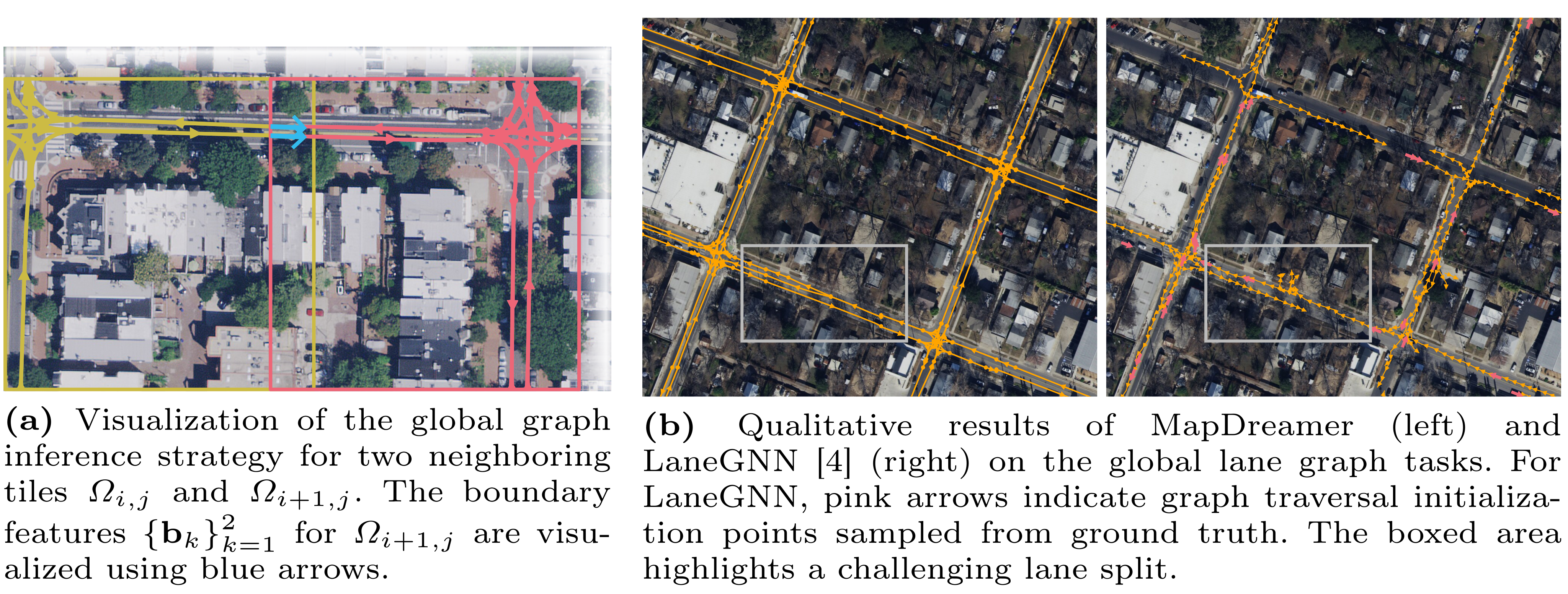
Global inference visits overlapping tiles from bottom-left to top-right. Each current tile receives boundary-intersection positions, local tangents and side indicators from the accumulated neighboring graph through a dedicated attention branch. Training sometimes drops left or bottom context to simulate one-neighbor cases, otherwise providing the L-shaped two-neighbor context.
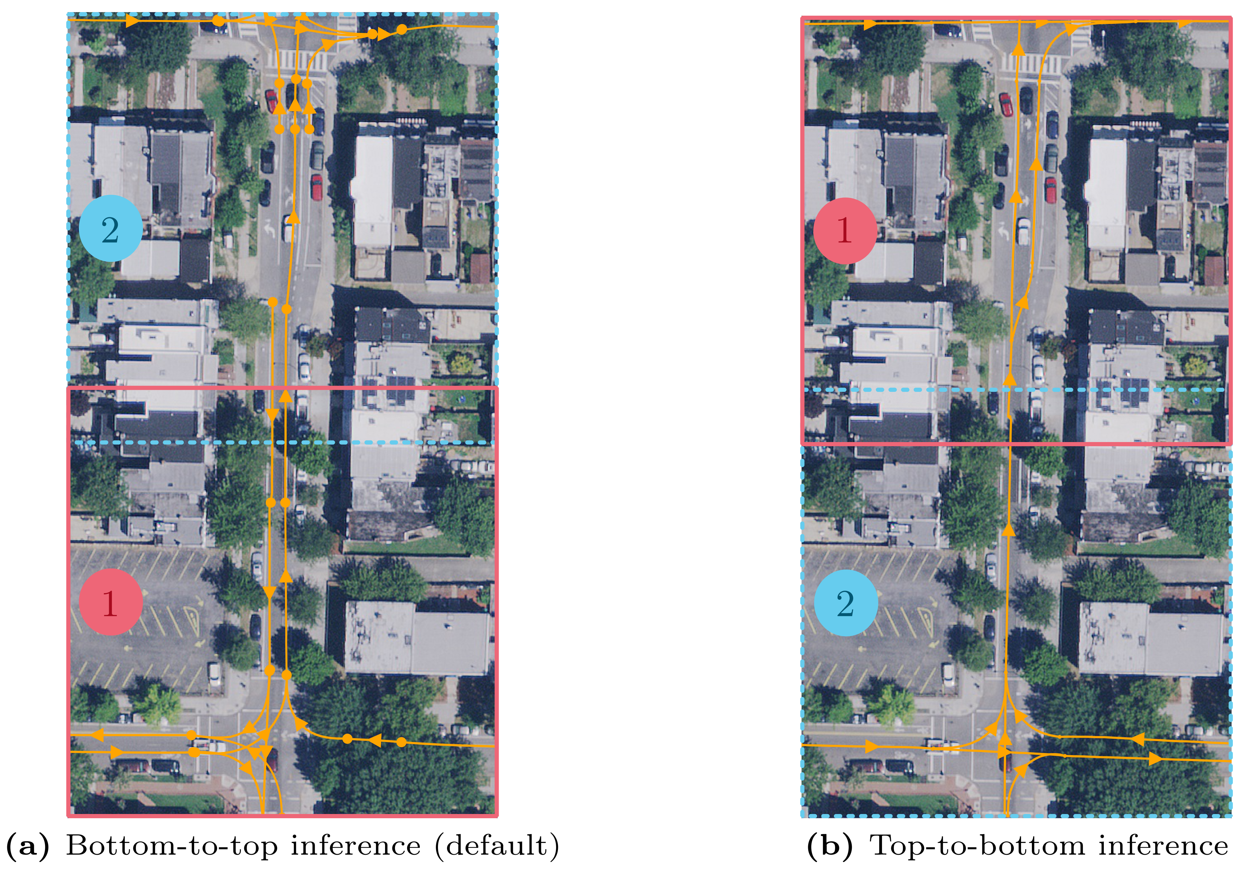
This compact conditioning replaces overlap inpainting, which the authors found vulnerable to accumulated mistakes. It still inherits earlier predictions: Appendix B demonstrates a wrong road direction propagated by the default order, corrected by starting from the tile that contains the decisive one-way marking.
Equation 9
| (9) |
4 Experiments
4.1 Data
The dataset combines Argoverse 2 maps with UrbanLaneGraph aerial imagery and geospatial train/validation regions. Spatial-redundancy filtering yields about 82,000 training and 1,200 validation samples, with within-split maximum overlap thresholds 0.8 and 0.4. The authors realign separate 2×2 km chunks and jointly rotate/translate images and graphs. Rejection sampling prevents missing-map boundary terminations from being moved into a training crop.
4.2 Metrics
GEO samples four centerline points per metre and performs one-to-one geometric matching, requiring distance within 1.2 or 2 metres and tangent disagreement no more than sixty degrees. Precision, recall and F1 thus penalize direction errors as well as misplaced geometry.
TOPO uses ground-truth topology to select junction-focused subgraphs: starts ten metres before splits, traverses fifty metres, reverses for merges, and also samples degree-one and long straight sections. GEO on those subgraphs measures local connectivity fidelity, not guaranteed city-wide route correctness. Raster IoU compares centerlines drawn at width twice the matching radius.
4.3 Results
BGFormer is retrained and reported at its best of three runs. LaneGNN uses supplied checkpoints, but its unreproduced LaneExtraction initialization is replaced by 178 poses sampled from ground truth for each global tile. It is excluded from local evaluation because that interface requires an oriented lane at the crop’s bottom center. No run-variation intervals are reported.
Local Lane Graph Evaluation.
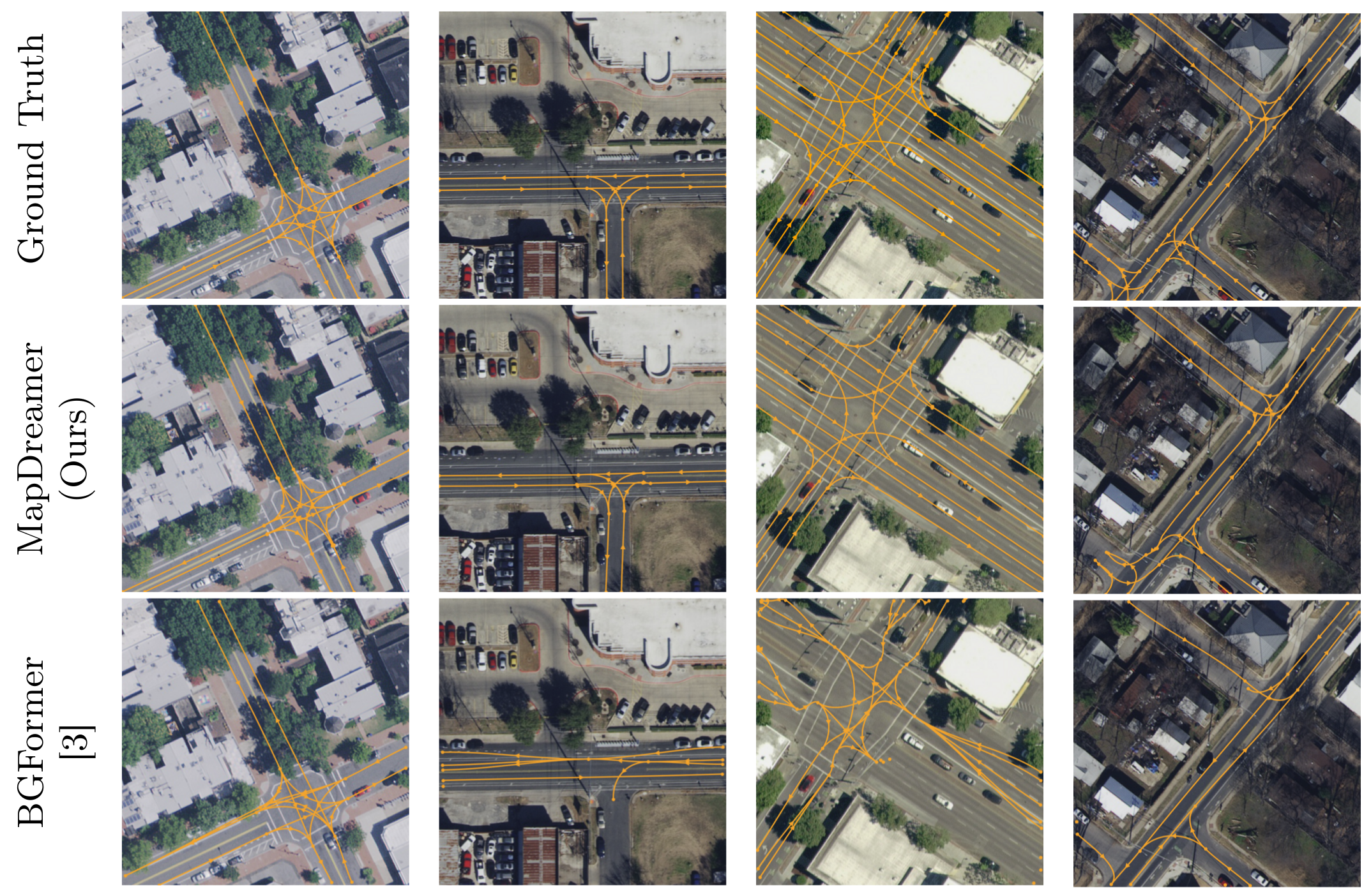
At the strict radius, MapDreamer’s local GEO F1 is 0.640 versus 0.458, TOPO F1 0.562 versus 0.345 and IoU 0.482 versus 0.354. Relaxed GEO/TOPO F1 are 0.768/0.702 versus 0.596/0.496. The paper’s 18.2% GEO gain denotes an absolute 0.182 difference, or 18.2 percentage points, rather than an 18.2% relative increase. The qualitative panels show improved selected junctions without establishing failure-free mapping.
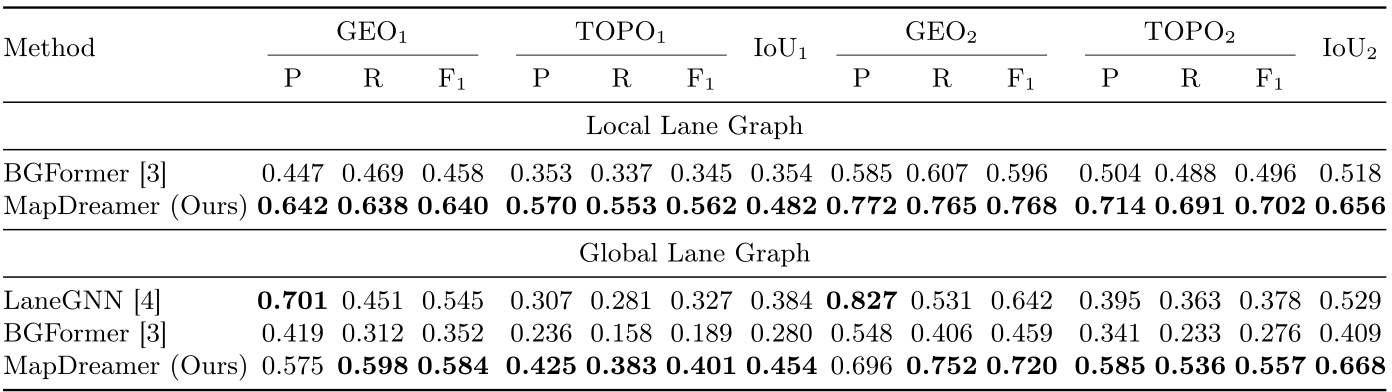
Original selectable table
| Method | ||||||||||||||||
| Local Lane Graph | ||||||||||||||||
| BGFormer [3] | 0.447 | 0.469 | 0.458 | 0.353 | 0.337 | 0.345 | 0.354 | 0.585 | 0.607 | 0.596 | 0.504 | 0.488 | 0.496 | 0.518 | ||
| MapDreamer (Ours) | 0.642 | 0.638 | 0.640 | 0.570 | 0.553 | 0.562 | 0.482 | 0.772 | 0.765 | 0.768 | 0.714 | 0.691 | 0.702 | 0.656 | ||
| Global Lane Graph | ||||||||||||||||
| LaneGNN [4] | 0.701 | 0.451 | 0.545 | 0.307 | 0.281 | 0.327 | 0.384 | 0.827 | 0.531 | 0.642 | 0.395 | 0.363 | 0.378 | 0.529 | ||
| BGFormer [3] | 0.419 | 0.312 | 0.352 | 0.236 | 0.158 | 0.189 | 0.280 | 0.548 | 0.406 | 0.459 | 0.341 | 0.233 | 0.276 | 0.409 | ||
| MapDreamer (Ours) | 0.575 | 0.598 | 0.584 | 0.425 | 0.383 | 0.401 | 0.454 | 0.696 | 0.752 | 0.720 | 0.585 | 0.536 | 0.557 | 0.668 | ||
Global Lane Graph Evaluation.
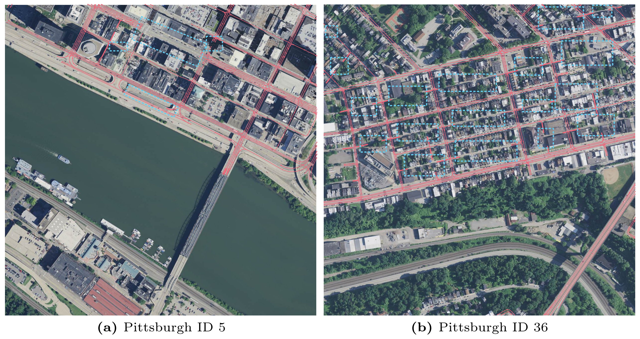
Global inference uses 5000×5000 evaluation tiles and rejects a 32-pixel margin around local predictions. Reported strict GEO F1 is 0.584 versus LaneGNN 0.545 and BGFormer 0.352. MapDreamer has higher recall but lower GEO precision than LaneGNN, so it does not dominate every metric. The headline means exclude the two Pittsburgh tiles because of identified annotation issues.
A source inconsistency affects the topology comparison: Table 1 prints LaneGNN precision 0.307, recall 0.281 and F1 0.327, while Table S1 reports its nine-tile mean F1 as 0.292. The printed F1 exceeds both main-table precision and recall. MapDreamer’s 0.401 therefore differs by 0.074 using Table 1, but 0.109 using Table S1; both source tables are retained without choosing an undocumented correction.
Failure Cases.
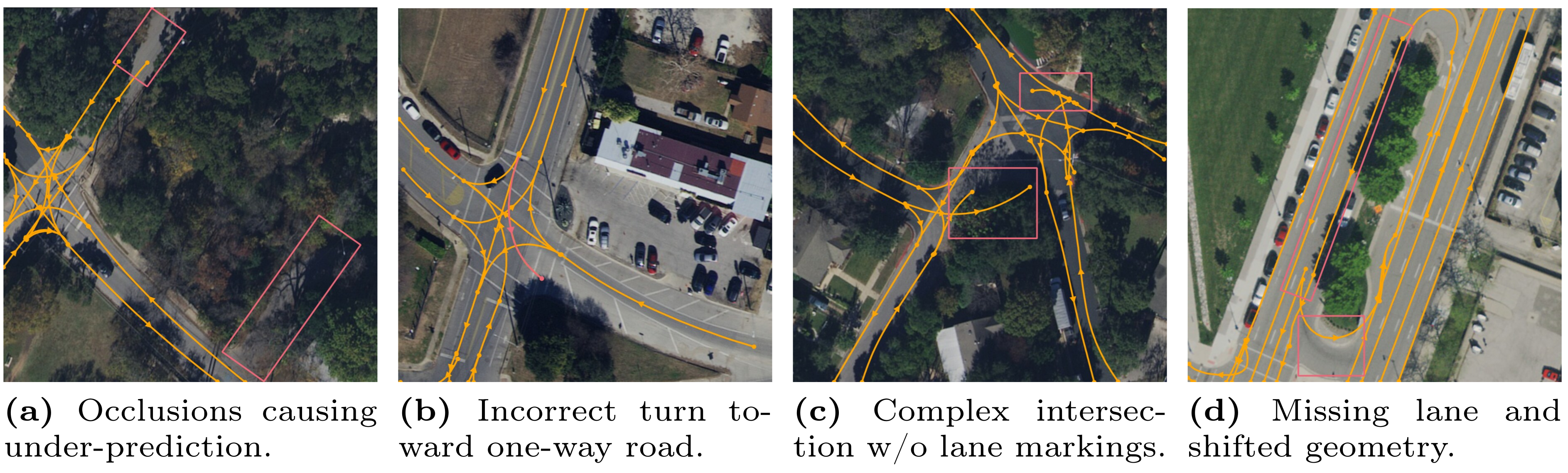
Heavy occlusion and absent markings can hide true lanes or induce plausible but wrong turns; unusual intersections and U-turns remain difficult. Better training coverage is proposed, not experimentally shown to eliminate these errors. These examples delimit the learned prior’s reliability where image evidence is weak.
4.4 Ablations
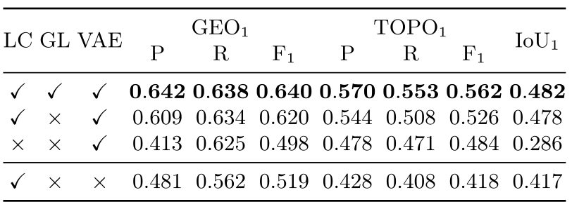
Ablations reuse one VAE checkpoint where applicable and compare lane cardinality, ghost capacity and latent versus direct-coordinate diffusion. Their numerical effects concern these model/training choices, not independent guarantees for every scene.
Ghost Lane Latents and Lane Cardinality.
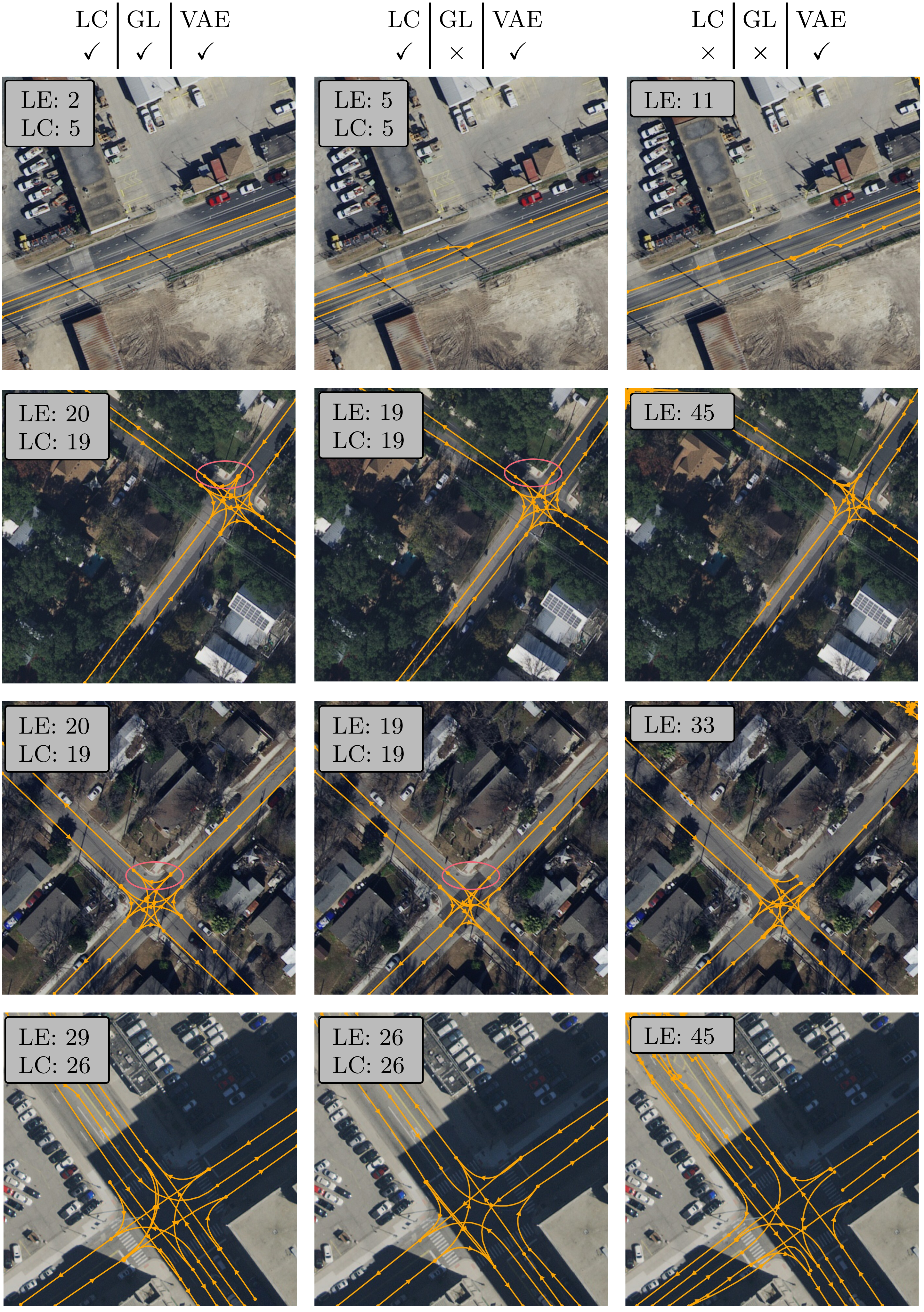
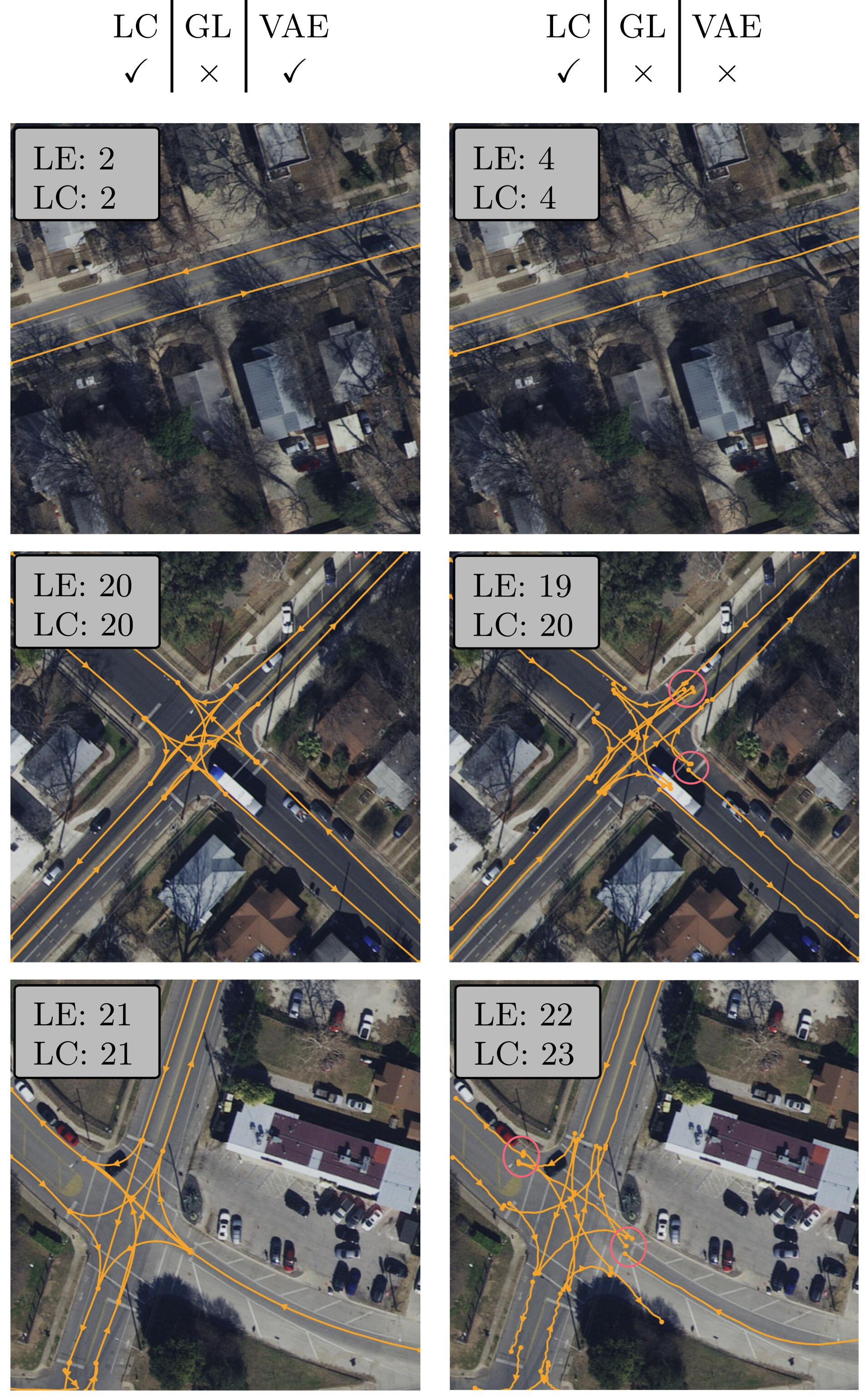
Removing ghosts reduces local GEO F1 from 0.640 to 0.620 and TOPO F1 from 0.562 to 0.526, principally through weaker precision and connectivity recall. Removing both ghosts and count prediction uses sixty-four fixed tokens; GEO precision falls from 0.642 to 0.413 while recall remains 0.625. Surplus tokens can survive existence filtering as duplicate lanes, consistent with the qualitative examples.
Vectorized Diffusion Model.
The direct-coordinate variant removes the VAE and adds a similarly sized topology head. Comparing the two no-ghost rows, GEO F1 falls from 0.620 to 0.519 and TOPO F1 from 0.526 to 0.418. This supports the latent representation under the tested setup; it does not isolate a mathematically enforced topology property. Appendix examples show less smooth geometry and poorer endpoint alignment.
Model Efficiency.
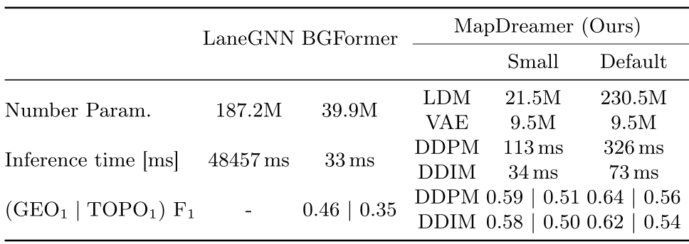
On a V100, default 100-step DDPM takes 326 ms per local tile; twenty-step DDIM takes 73 ms with GEO/TOPO F1 about 0.62/0.54 versus 0.64/0.56. The small variant reduces hidden width 2048→512 and reaches 34 ms with DDIM, close to BGFormer’s 33 ms, at about 0.58/0.50 versus 0.46/0.35.
Table 3 counts trainable inference parameters: small/default LDM 21.5M/230.5M plus 9.5M VAE, excluding frozen-backbone parameters from that stated count. LaneGNN’s 48,457 ms is global-run time normalized by tile-area ratio, not the same directly timed local interface. Sliding-window aggregation and sequential dependencies also limit extrapolation from local latency to city-wide throughput.
5 Conclusion
Aerial-conditioned latent diffusion improves the tested lane-graph reconstruction metrics and can stitch large map tiles with directed boundary context. The demonstrated scope remains centerlines and their relations on curated six-city data. Lane boundaries, crossings, complementary vehicle trajectories, adaptive inference order and faster flow-matching generation are future directions. Neither benchmark improvements nor generative plausibility certify safe navigation.
Supplementary Material
The supplement documents data curation, all eleven global evaluation tiles, large qualitative panels, ablations and model/optimizer settings. Its excluded-city results and filtering details are essential context for the main averages.
Appendix 0.A Dataset
Overhead lane-level datasets are less common than vehicle-view mapping datasets. The authors choose a larger aligned aerial/map source, then curate local crops rather than using every Argoverse scenario unchanged.
0.A.1 Available Datasets
UrbanLaneGraph covers Austin, Miami, Pittsburgh, Palo Alto, Detroit and Washington DC, with 5,223.3 km of lane annotations versus LaneExtraction’s 398.6 km. This motivates dataset choice; it is annotation coverage, not the total extent of independently evaluated city-scale maps.
0.A.2 MapDreamer Dataset
Filtering starts from 250,000 Argoverse Motion Forecasting scenarios and retains extra surrounding context for crop augmentation. Overlap thresholds differ between training and validation, while the geospatial split prevents region sharing. The resulting sample counts are the approximately 82,000/1,200 reported in the main text.
Map Alignment.
The original city alignment uses three correspondences and a Kabsch–Umeyama transformation. MapDreamer instead aligns 2×2 km chunks separately to reduce local map/image mismatch. This refinement is part of data preparation; the model is not demonstrated to infer arbitrary georegistration itself.
Appendix 0.B Extended Results
Full-tile results reveal substantial geographic variation, annotation problems and boundary-order effects hidden by aggregate scores. All large source panels and their marked failure regions are retained.
0.B.1 Global Lane Graph Evaluation
Quantitative Results.
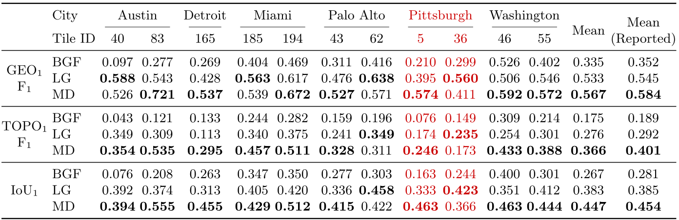
Table S1 reports all eleven tiles and a separate nine-tile mean excluding Pittsburgh IDs 5 and 36. Across all eleven, MapDreamer GEO/TOPO F1 are 0.567/0.366 versus LaneGNN 0.533/0.276 and BGFormer 0.335/0.175. The reported nine-tile values are 0.584/0.401, 0.545/0.292 and 0.352/0.189, respectively.
Individual tiles are mixed: LaneGNN leads GEO F1 on several tiles and TOPO F1 on Palo Alto 62 and Pittsburgh 36. Figure S1 identifies ground-truth continuity problems rather than independently proving every model output correct. Table S1’s LaneGNN topology mean conflicts with Table 1; minor IoU rounding/reporting differences also remain in the exact tables.
Original selectable table
| City | Austin | Detroit | Miami | Palo Alto | Pittsburgh | Washington | ||||||||||||||
|---|---|---|---|---|---|---|---|---|---|---|---|---|---|---|---|---|---|---|---|---|
| Tile ID | 40 | 83 | 165 | 185 | 194 | 43 | 62 | 5 | 36 | 46 | 55 | Mean | Mean (Reported) | |||||||
| BGF | 0.097 | 0.277 | 0.269 | 0.404 | 0.469 | 0.311 | 0.416 | 0.210 | 0.299 | 0.526 | 0.402 | 0.335 | 0.352 | |||||||
| LG | 0.588 | 0.543 | 0.428 | 0.563 | 0.617 | 0.476 | 0.638 | 0.395 | 0.560 | 0.506 | 0.546 | 0.533 | 0.545 | |||||||
| MD | 0.526 | 0.721 | 0.537 | 0.539 | 0.672 | 0.527 | 0.571 | 0.574 | 0.411 | 0.592 | 0.572 | 0.567 | 0.584 | |||||||
| BGF | 0.043 | 0.121 | 0.133 | 0.244 | 0.282 | 0.159 | 0.196 | 0.076 | 0.149 | 0.309 | 0.214 | 0.175 | 0.189 | |||||||
| LG | 0.349 | 0.309 | 0.113 | 0.340 | 0.375 | 0.241 | 0.349 | 0.174 | 0.235 | 0.254 | 0.301 | 0.276 | 0.292 | |||||||
| MD | 0.354 | 0.535 | 0.295 | 0.457 | 0.511 | 0.328 | 0.311 | 0.246 | 0.173 | 0.433 | 0.388 | 0.366 | 0.401 | |||||||
| BGF | 0.076 | 0.208 | 0.263 | 0.347 | 0.350 | 0.277 | 0.303 | 0.163 | 0.244 | 0.400 | 0.301 | 0.267 | 0.281 | |||||||
| LG | 0.392 | 0.374 | 0.313 | 0.405 | 0.420 | 0.336 | 0.458 | 0.333 | 0.423 | 0.351 | 0.412 | 0.383 | 0.385 | |||||||
| MD | 0.394 | 0.555 | 0.455 | 0.429 | 0.512 | 0.415 | 0.422 | 0.463 | 0.366 | 0.463 | 0.444 | 0.447 | 0.454 | |||||||
Qualitative Results.
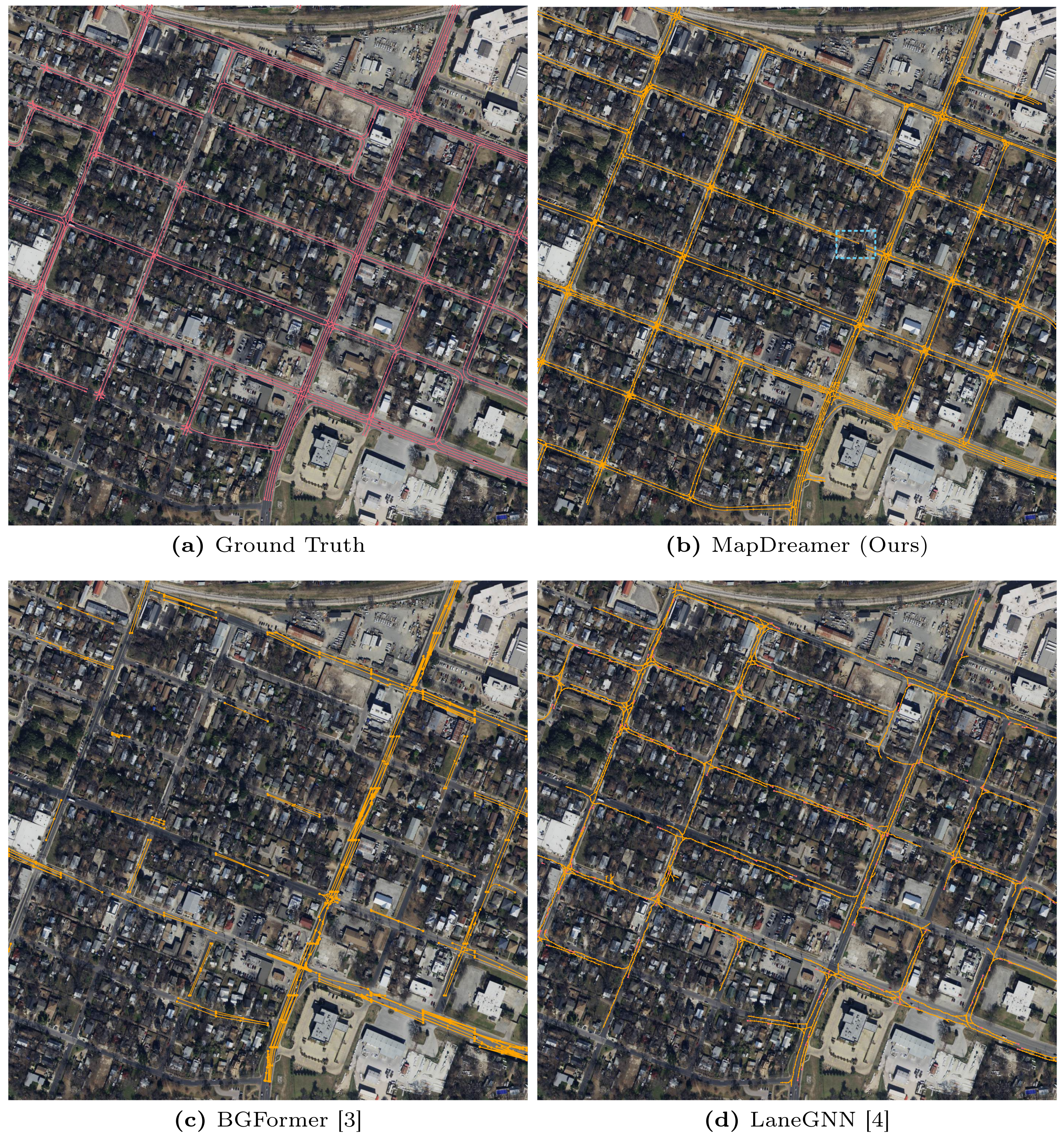
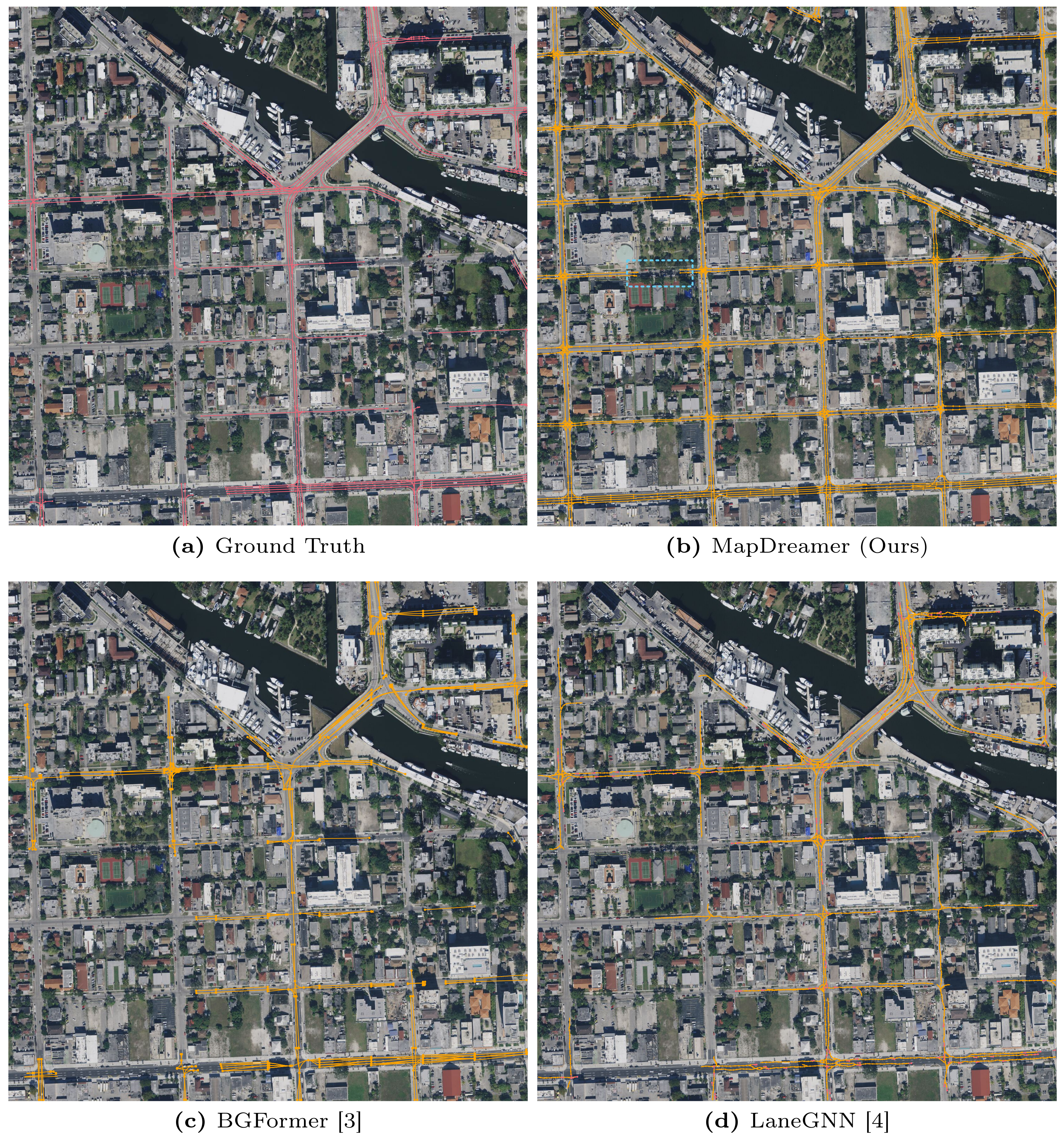
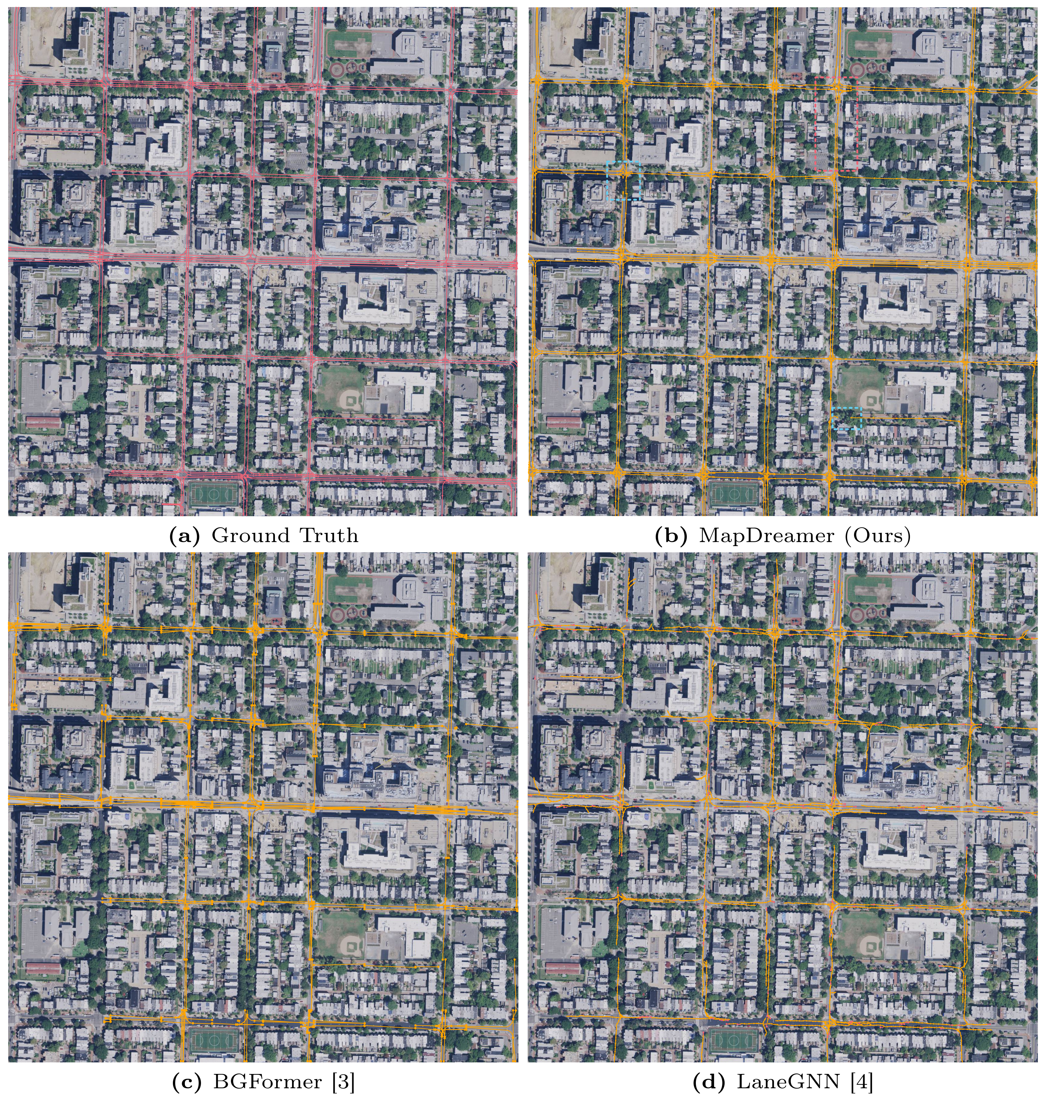
Figures S2–S4 retain complete Austin 83, Miami 185 and Washington 46 map panels, with ground truth, MapDreamer, BGFormer and LaneGNN. Baseline visualizations discard predictions farther than fifty pixels from ground-truth support, whereas MapDreamer visualizations retain all predictions. Quantitative metrics apply the same correspondence filtering to all methods. Thus displayed coverage is not filtered identically, and reported scores assess the annotated support region rather than unrestricted map completeness.
Failure Modes.
Cyan boxes mark breaks under trees, shadows and buildings. The Washington example exposes ordering sensitivity: bottom-up generation commits to an incorrect two-way road before seeing a one-way arrow, then passes that mistake to the next tile. Reversing the order sees the marking first and continues the correct one-way interpretation. Boundary conditioning promotes consistency with prior predictions, which can include consistent errors.
0.B.2 Ablations
Lane Cardinality and Ghost Lane Latents.
Figure S6 shows count correction in selected cases: a five-lane estimate becomes two retained lanes, nineteen becomes twenty, and twenty-six becomes twenty-nine. The no-ghost examples keep the estimated count, while fixed-budget variants overgenerate. These illustrations support the finite spare-capacity mechanism; they do not establish perfect count calibration or prove that every existence head always follows its counter.
Original selectable diagram symbols
Vectorized Diffusion Model.
Figure S7 compares latent and direct-coordinate diffusion without ghosts. Simpler geometry is plausible for both, but difficult intersections expose rough curves and endpoint mismatch in the coordinate variant. The small qualitative selection complements the table’s metric losses; changes in predicted counts and geometry both contribute.
Original selectable diagram symbols
Appendix 0.C Implementation Details
The VAE uses two encoder/two decoder blocks, geometry width 512, connectivity width 64 and latent dimension 24. Geometry, connectivity and endpoint loss weights are each ten. Both LDM sizes have two blocks, with geometry width 2048 or 512.
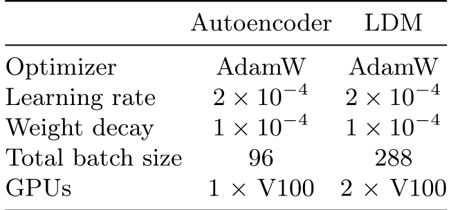
Both stages use AdamW at learning rate 2×10⁻⁴ and weight decay 10⁻⁴. Total batch sizes are 96 for the autoencoder on one V100 and 288 for diffusion on two V100s. The supplied tables do not specify a complete training duration, KL weight, guidance scale or existence threshold, so these notes do not invent them.
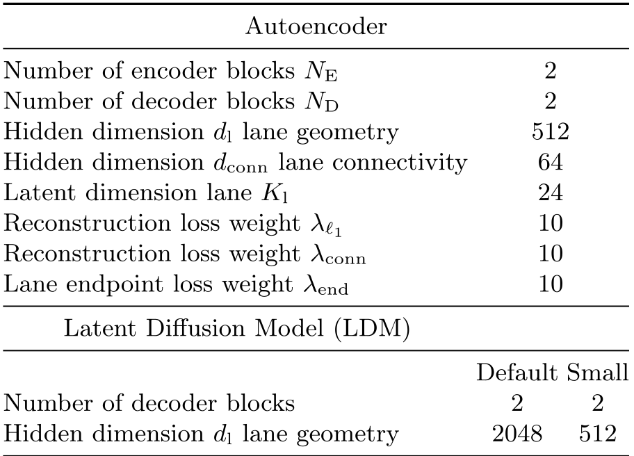
Original selectable table
| Autoencoder | ||
|---|---|---|
| Number of encoder blocks | 2 | |
| Number of decoder blocks | 2 | |
| Hidden dimension lane geometry | 512 | |
| Hidden dimension lane connectivity | 64 | |
| Latent dimension lane | 24 | |
| Reconstruction loss weight | 10 | |
| Reconstruction loss weight | 10 | |
| Lane endpoint loss weight | 10 | |
| Latent Diffusion Model (LDM) | ||
| Default | Small | |
| Number of decoder blocks | 2 | 2 |
| Hidden dimension lane geometry | 2048 | 512 |