At a glance
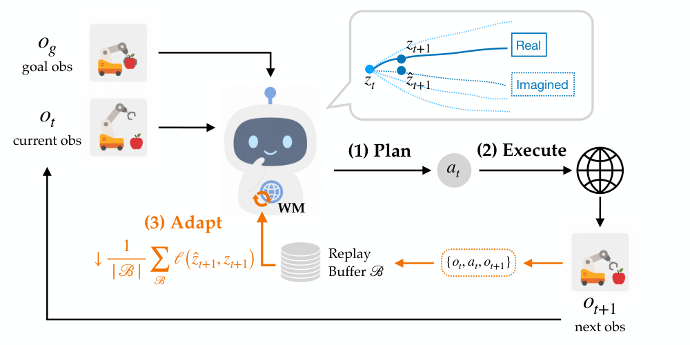
A planner can keep making poor choices if its internal model stays wrong. AdaJEPA closes that feedback loop: plan with the current world model, execute a short action chunk, observe what actually happened, update the model, and plan again. The update uses prediction error from the new transition, without a new expert demonstration or reward label. In the tested simulated tasks, updating only a few layers for one gradient step often improves goal reaching at small additional cost. Each episode starts from the same pretrained checkpoint. This is lightweight within-episode adaptation, not a guarantee of unlimited continual learning or arbitrary distribution-shift recovery.
1 Introduction
A frozen world model can mispredict the consequences of actions, and planning may amplify those errors. The proposed remedy uses the very transitions produced during control as new self-supervised training examples. It complements offline pretraining by correcting the model locally while the agent acts.
2 Related Work
JEPA world models.
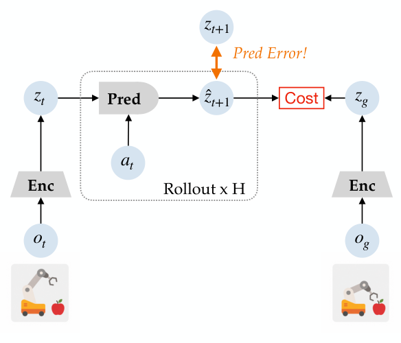
JEPA world models predict future features instead of pixels. Goal-conditioned control then searches for actions that bring those features near an encoded goal. Their learned representations, dynamics predictors and anti-collapse objectives can vary.
Test-time training and adaptation.
Test-time adaptation changes a trained model using information available during deployment. AdaJEPA applies this idea to action-conditioned feature prediction, using the observed next state as a target.
Adaptation in planning and control.
Adaptive control and online model-based learning provide earlier versions of the same broad feedback principle. AdaJEPA places small model updates directly inside a pretrained latent model’s planning loop, without a separate target-domain demonstration phase.
3 AdaJEPA: An Adaptive Latent World Model
The method repeats plan, execute, observe, adapt and replan. Updating the dynamics or visual representation changes the model that the next planning problem uses. The original algorithm gives the full episode procedure.
3.1 Background: JEPA World Models
An image encoder describes the state, an action encoder describes the command, and a predictor forecasts the next representation. Offline training minimizes future-feature error with a stabilizer against collapse. Planning rolls out candidate actions and minimizes a goal-distance cost. Prediction quality and the geometry of that cost both affect success.
Equations 1–3
| (1) |
| (2) |
| (3) |
3.2 Closed-Loop Plan-and-Adapt
After each executed action chunk, the observed transition supplies a small training update before the next plan. Each episode has its own model copy and replay buffer, reset from the pretrained checkpoint at the start. Adaptation uses interaction data, even though it requires no additional expert answers.
Online buffer.
A bounded buffer keeps recent transitions or transitions with the largest prediction error. Recent data focus the update on the local situation the controller is currently encountering. The buffer is an adaptation memory, separate from the offline training dataset.
Adaptation loss.
The adaptation loss again compares predicted and observed latent targets. The default stops gradients through the target branch, while updating a restricted parameter subset. This is a practical stabilization recipe; the limited-update ablation is evidence about the tested models, not a general proof that online collapse cannot occur.
Equation 4
| (4) |
Equation
Adapted parameters.
Only a selected subset of encoder and predictor parameters needs to change. A few gradient updates are then immediately reused for planning. Restricting the update makes adaptation cheaper and reduces how far it can move from the pretrained model.
Equation 5
| (5) |
4 Experiments
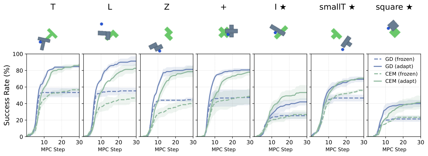
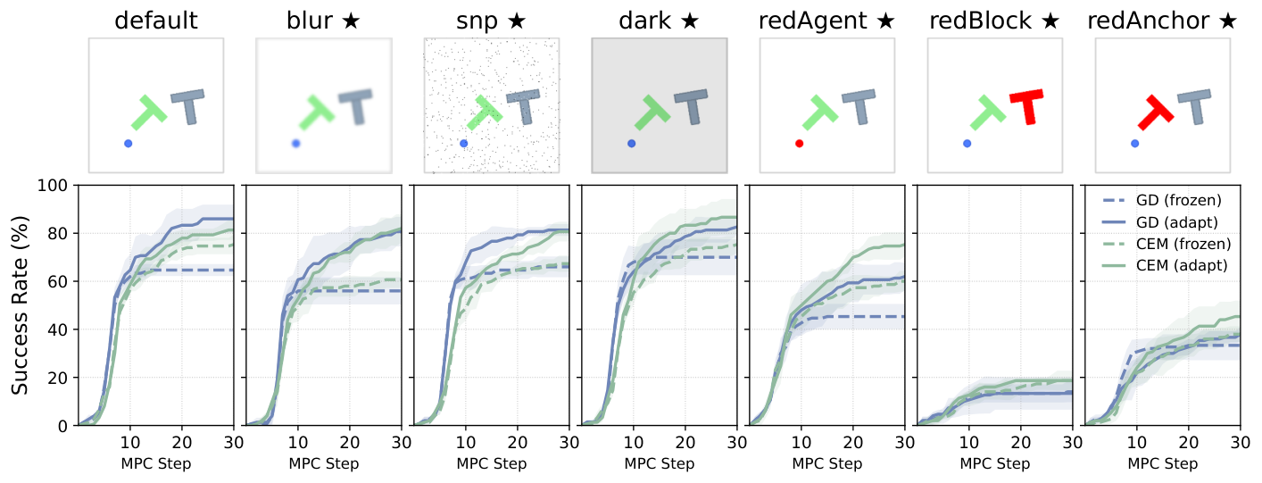
Experiments compare adaptive and frozen versions of the same world model under controlled changes in geometry, appearance, physics and maze layout. The evidence concerns these simulated goal-reaching tasks and their planning protocols.
4.1 Setup
Environments.
PushObj changes object shape while retaining the underlying contact setting. PushT tests image corruptions and color changes. PointMaze changes mass, damping or maze layout. Training and test sets separate the specified conditions; these are distinct kinds of shift, not one unrestricted out-of-distribution benchmark.
Plan-and-Adapt.
The default update changes the last visual-encoder and predictor layers once per replan, using five recent transitions and the training learning rates. Results average several test seeds and episodes. The source uses different 20- and 30-replan budgets across experiments; its captions and appendix settings should accompany reproduced scores.
Equation
Architectures.
The main models combine a small residual encoder, action and proprioceptive inputs (measurements of the agent’s own state), and a transformer predictor. Stop-gradient and a regularizer favoring straighter latent trajectories are part of the pretraining recipe. Additional comparisons apply the adaptation loop to other world-model implementations.
4.2 Results
In-distribution performance.
Adaptation improves several in-distribution cases where the frozen model is imperfect and preserves performance in the strong tested baseline. This supports applying the method in those experiments; it does not establish that adaptation is universally harmless.
Distribution shifts.
The reported shifts generally benefit from adaptation, including new shapes and maze layouts. Some color changes yield only modest gains because color helps distinguish the object from the reference. Recovering from a mismatch in visual features can require encoder updates as well as predictor updates.
| Dynamics Shift (PointMaze-Medium) | Layout Shift | |||||||||||||||||||||||
| default | low mass | high damping | Unseen Layouts | |||||||||||||||||||||
| Adapt | GD | CEM | GD | CEM | GD | CEM | GD | CEM | ||||||||||||||||
| Frozen | 82.7 | 6.8 | 84.0 | 3.3 | 77.3 | 8.2 | 82.0 | 2.8 | 77.3 | 5.0 | 76.0 | 2.8 | 53.3 | 8.2 | 49.3 | 6.2 | ||||||||
| predlast + enclast | 83.3 | 6.6 | 0.7 | 83.3 | 3.4 | 0.7 | 80.0 | 3.3 | 2.7 | 86.7 | 2.5 | 4.7 | 77.3 | 10.5 | 78.7 | 3.4 | 2.7 | 66.0 | 7.1 | 12.7 | 55.3 | 5.0 | 6.0 | |
| predfirst + enclast | 84.0 | 1.6 | 1.3 | 84.0 | 4.3 | 82.0 | 1.6 | 4.7 | 82.7 | 3.4 | 0.7 | 78.7 | 4.7 | 1.3 | 82.0 | 3.3 | 6.0 | 78.7 | 5.0 | 25.3 | 70.7 | 3.8 | 21.3 | |
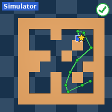
frozen success
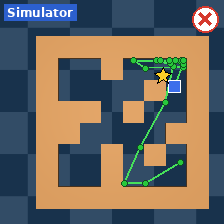
frozen failure
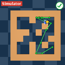
adapt success
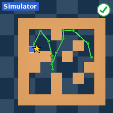
frozen success
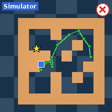
frozen failure
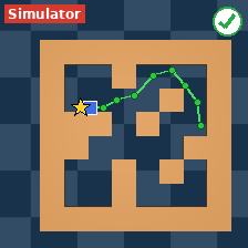
adapt success
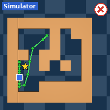
frozen failure
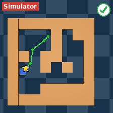
adapt success
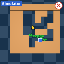
frozen failure
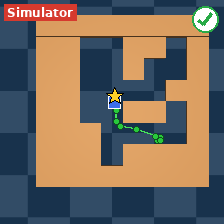
adapt success
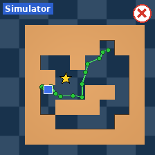
frozen failure
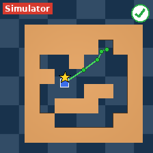
adapt success
Latency.
A small selected-layer update adds little measured time per replan in the tested implementations. Reaching the goal with fewer replans can compensate for that overhead. The latency result depends on the model, planner, hardware and number of update steps.
Visualization.
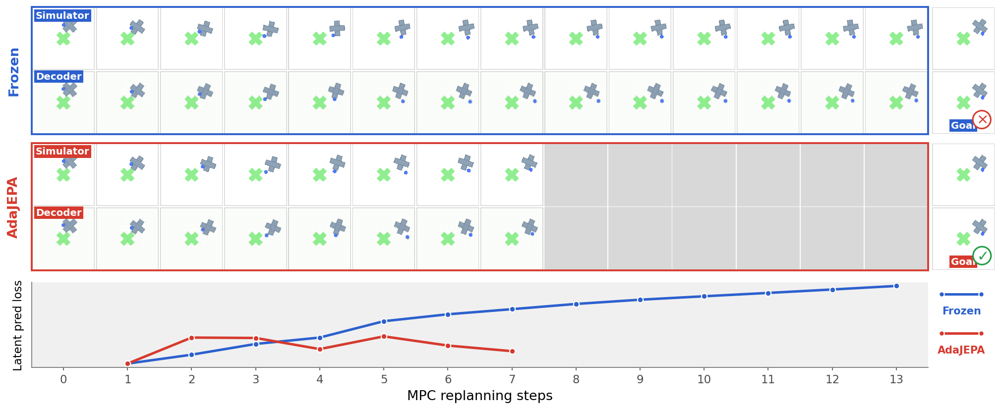
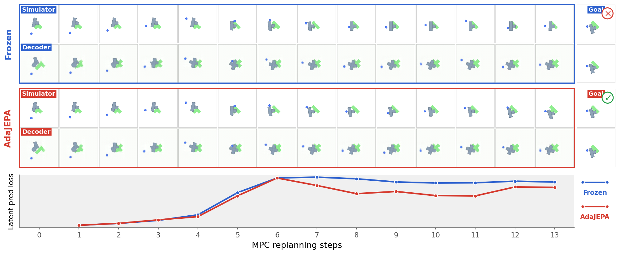
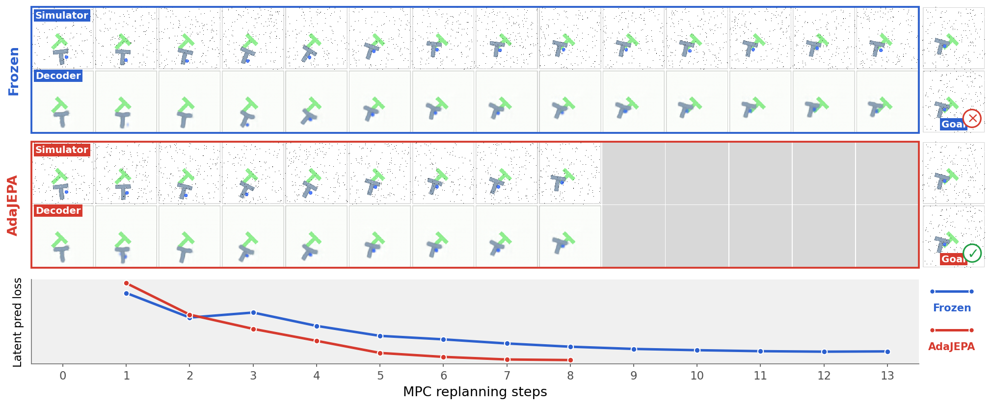
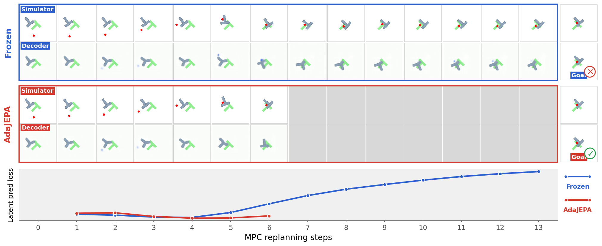
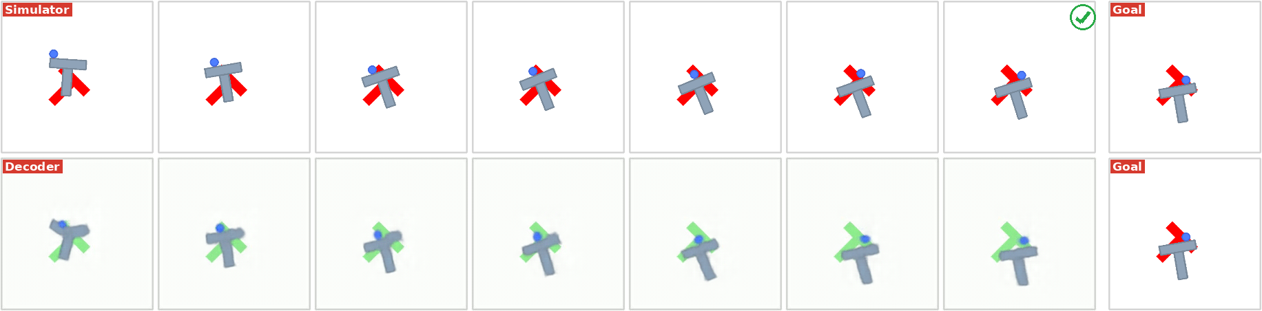
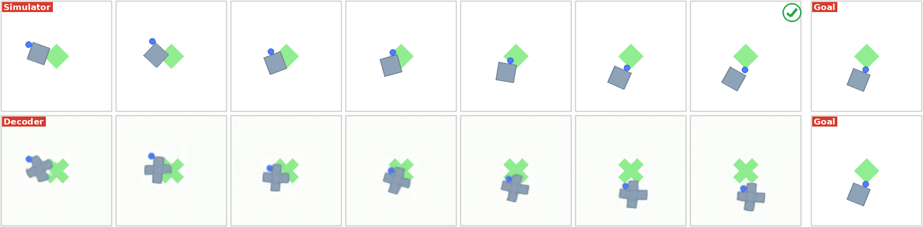
A separate decoder visualizes imagined latent rollouts. It can reconstruct training-like colors or shapes even when the observed test image differs. These examples suggest the updates reuse existing latent structure; decoding is an analysis tool, not part of the goal-reaching objective.
| Encoder / Predictor | Latent Dim | Anti-collapse | Setting | GD (%) | Time (s) | CEM (%) | Time (s) | ||||
|---|---|---|---|---|---|---|---|---|---|---|---|
| WM w/ Temporal Straightening | stop-grad | Frozen | 84.0 | 2.0 | 3.14 | 74.0 | 3.5 | 0.24 | |||
| (global feat.) (Wang et al., 2026) | Adapt | 85.3 | 3.1 1.3 | 3.17 | 0.03 | 81.3 | 6.4 7.3 | 0.27 | 0.03 | ||
| WM w/ Temporal Straightening | stop-grad | Frozen | 91.3 | 4.2 | 3.37 | 89.3 | 3.1 | 5.37 | |||
| (spatial feat.) (Wang et al., 2026) | Adapt | 92.0 | 3.5 0.7 | 3.38 | 0.01 | 93.3 | 2.3 4.0 | 5.39 | 0.02 | ||
| DINO-WM (patch) | - | Frozen | 68.0 | 10.6 | 3.66 | 86.7 | 6.1 | 9.53 | |||
| (spatial feat.) (Zhou et al., 2025) | Adapt | 70.0 | 4.0 2.0 | 3.68 | 0.02 | 90.0 | 3.5 3.3 | 9.56 | 0.03 | ||
4.3 Ablations
Which parameters to adapt?
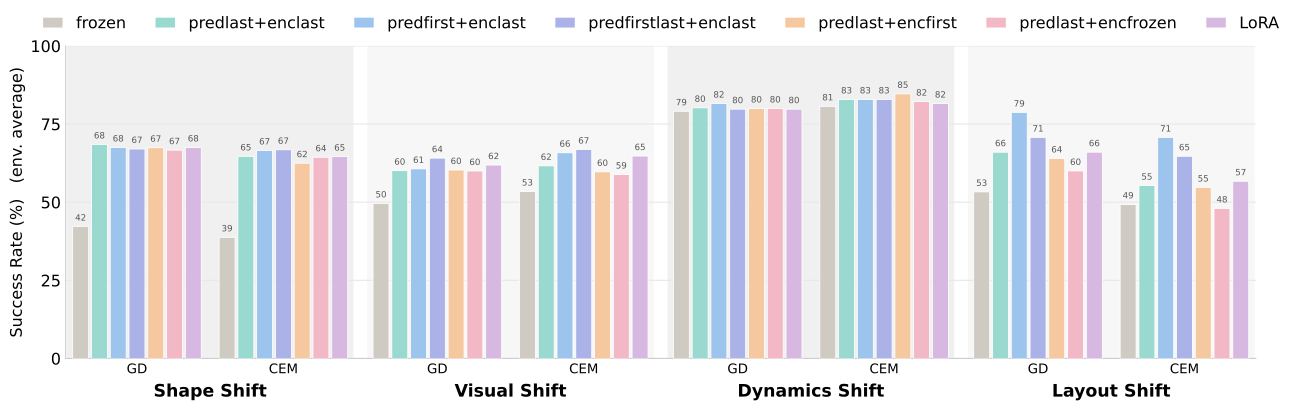
Several selected-layer and low-rank-adapter updates improve on the frozen baseline. Shape changes can often be handled mainly by the predictor, whereas visual and layout changes benefit from encoder adaptation too. The best target depends on the environment; the experiment does not identify one universally optimal layer.
How should adaptation hyperparameters be chosen?
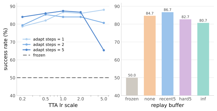
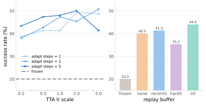
One step at the training learning rate is a useful tested default. Larger rates can work with one step but overshoot with repeated updates; smaller rates may need more steps. Buffer design has a smaller effect in these ablations. Stronger adaptation trades extra cost and possible instability for more correction.
AdaJEPA improves over various JEPA world models.
The loop improves the evaluated world models across several architectures, representation layouts and planners. Reported added time is about 0.01–0.03 seconds per replan for these models. This shows portability across the tested implementations rather than an architecture-independent guarantee.
4.4 Discussion
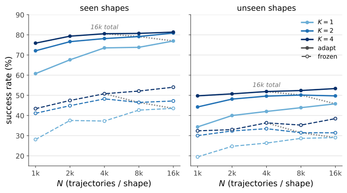
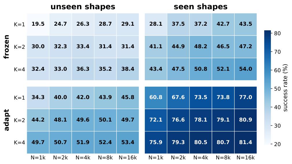
More training data and greater shape diversity help both frozen and adaptive models. Adaptation is particularly valuable when coverage is limited, but cannot reliably manufacture features the pretrained representation never learned. The data-scale study therefore supports combining pretraining and online correction, rather than replacing either with the other.
(a) PushT-RedAnchor
(b) PushObj-Square
5 Conclusion
Small self-supervised updates inside the control loop can correct useful prediction errors while the agent acts. The demonstrated benefit is within-episode simulated planning. Extending representation coverage through longer-term active or continual learning remains a proposed next step.
Acknowledgments
The authors acknowledge research funding, computing support and discussions that contributed to the work.
Appendix A Environments and Data
A.1 PushT (DINO-WM)
The PushT task moves a T-shaped block toward a target pose. In the DINO-WM evaluation setup, the fixed green T is a visual reference rather than the manipulated target object. This distinction matters for interpreting the color-shift experiments.
A.2 PushObj
PushObj replaces the block with several shapes. Replaying old actions can miss a new shape, so the dataset is biased toward contact and test trajectories require at least one contact. Shape-shift and visual-shift experiments use different training subsets. Their results depend on this deliberately contact-rich sampling.
A.3 PointMaze-Medium
PointMaze-Medium applies forces to a moving agent in a fixed maze. Tests alter mass or damping and choose separated start/goal cells, reducing trivial short-distance cases. The experiment reuses the cited pretrained model and data.
A.4 Diverse PointMaze
The layout test trains on 25 generated mazes and holds out five. Goals are selected three to five shortest-path cells away using breadth-first search. This tests new layouts with the specified generation and distance rules.
Appendix B Experiments
B.1 Hyperparameters
The retained tables give the full model, training and planning hyperparameters. Keep these together with the data and evaluation budget when reproducing an adaptive-versus-frozen comparison.
| Name | Value |
|---|---|
| Encoder lr | 1e-5 |
| Predictor lr | 5e-4 |
| Action/Prop encoder lr | 5e-4 |
| Batch size | 64 |
| History frames | 3 |
| Frameskip | 5 |
B.2 Ablations
These ablations vary the parameter subset, learning rate, update count and replay strategy while keeping the remaining protocol as consistent as specified.
Setup.
The encoder’s last stage is its projection head; its first stage extracts low-level visual features. Predictor variants update selected transformer blocks. The appendix uses a shorter replanning budget for these ablations than the longer-budget main plots.
What to adapt.
The listed variants change early or late predictor blocks, early or late encoder stages, or low-rank adapters while freezing the remaining parameters. Several choices work; stronger layout adaptation from early predictor changes suggests sensitivity near the state/action input interface.
Learning rates, optimization steps, and replay buffers.
Learning rate and update count interact: a large step can help quickly but repeated large steps may overshoot. Recent-transition buffers are a stable default in the tested grid, although adaptation also helps without a buffer. Best settings remain model- and environment-dependent.
B.3 Additional Experiments: Training Data Scale for PushObj
The data study varies both the number of shapes and trajectories per shape, balances which shapes appear in each training set, and holds optimization-step count fixed. Diversity improves generalization, while adaptation adds gains across the examined scales. Comparisons to larger frozen datasets use this specific training and evaluation design.
Appendix C Visualization of Planning Trajectories
The original panels compare observed trajectories, decoded imagined rollouts, goal success and prediction error over successive replans. Adaptive runs are grayed after reaching the goal; frozen runs are capped for display. A decoder trained on default images may retain their colors even when the real test observations change.