Overview
Read this as a throughput-oriented reconstruction of IPOPT for many independent nonlinear programs. The original diagrams, plots, tables and mathematical displays remain available alongside the condensed argument. The reviewed source is arXiv v2, dated 3 November 2026.
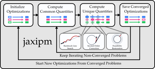
At a glance
jaxipm implements generally constrained nonlinear optimization in JAX so hundreds of independent problems can share one GPU. Heterogeneous iteration fusion preserves each problem’s branch choices within a uniform computation graph; iteration-level batching replaces finished problems immediately. Across three quadrotor control benchmarks, one L40S GPU delivers 30.7–69.9% of the throughput of 64 concurrent CPU IPOPT instances. The gain is over sequential solvers, while the 64-core baseline remains faster.
I Introduction
Sampling-based robot learning and control can run many simulations on a GPU, but embedding a conventional nonlinear-program solver introduces CPU calls and transfers. jaxipm rebuilds IPOPT’s interior-point algorithm around two sources of divergence: different fallback branches and different numbers of iterations. Shared expensive calculations run together; remaining branch-specific calculations run for all problems before selecting the appropriate outputs. Completed slots receive new problems at iteration boundaries. This supports constrained trajectory generation on the GPU; integration into a complete learning or sampling-based control pipeline remains future work.
II Related Works
Existing nonlinear solvers provide mature constraint handling on CPUs. GPU-accelerated approaches such as MadNLP/ExaModels move derivative evaluation and linear algebra to the GPU while retaining CPU control flow. Earlier batched solvers mainly address convex programs or much smaller bound-constrained nonconvex problems. jaxipm targets general nonlinear equality/inequality constraints with independent branch decisions across a batch. Optimization-generated imitation datasets motivate the application, but dataset-training gains are not evaluated here.
III Problem Statement
Each problem minimizes a twice-differentiable objective subject to twice-differentiable equalities and elementwise bounds; general inequalities enter through slack variables. A batch shares the objective/constraint structure and bounds while varying its parameters and initial conditions. Its decision variables remain independent, making it mathematically equivalent to separate solver calls. This is concurrent solution of many programs, rather than a coupled optimization over all samples.
| Predicate | True branch | Branch-unique computation |
| (1) Is the trial rejected? | Backtracking line search shortens the step and retests. This occurs repeatedly until a convergence condition is met. | Re-evaluation of and , filter acceptance test, reduction of . |
| (2) Does the trial have surprising characteristics? | A second-order correction changes the step direction based on information gathered at the original trial. This occurs repeatedly until a convergence condition is met. | Modified right hand side of Equation (3), solved against the existing factorization of the left hand side of Equation (3), re-evaluation of and . |
| (3) Is a short run of rejected iterates hiding longer-horizon progress? | The watchdog accepts a small sequence of trial steps unconditionally, either accepting the resultant trial, or reverting to the entry iterate. | Copy and restore of the reference iterate and direction, counters. Scalar and vector arithmetic only. |
| (4) Are the steps really small? | A tiny-step rule accepts it unconditionally. | A convergence check using scalar arithmetic at the current trial point only. |
| (5) Are there repeated trial rejections? | Soft feasibility restoration changes the acceptance criteria, and continues until original criteria are fulfilled or an iteration limit is reached. | Re-evaluation of , and their derivatives, acceptance test. |
| (6) Is the optimizer unable to make progress? | Hard feasibility restoration solves a new problem whose objective is the constraint violation, returning to the original problem once an acceptable point is found. | None beyond the shared work; the next iteration instantiates the restoration. |
| (7) Is the optimization unstable? | Barrier parameter update switches from an adaptive rule to a monotone schedule. | Both updates are computed for every member regardless of the update rule. Scalar arithmetic only. |
Equations 1a–2
| (1a) | ||||
| s.t. | (1b) | |||
| (1c) | ||||
| (2) |
IV IPOPT Background
IPOPT uses a shrinking logarithmic barrier, primal/dual variables and Newton steps from the constraint Jacobian and Lagrangian Hessian. Robustness requires backtracking, second-order corrections, watchdog steps, tiny-step acceptance, soft/hard feasibility restoration and alternative barrier updates. Table I preserves the conditions and work of every listed branch. Simply stacking problems into one larger IPOPT call forces shared branch choices and can increase iterations or cause failure; separate CPU calls retain independent branches but do not exploit a single GPU batch.
Equations 3
| (3) |
V Batched Interior-Point Method
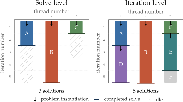
The implementation computes shared functions, derivatives, Newton steps and fraction-to-boundary quantities once per iteration. It evaluates the remaining branch-specific work unconditionally and selects results by each problem’s predicate. Padding makes the ordinary and nested hard-restoration problems share a computation graph. Conditional line-search and second-order-correction loops continue across the batch until every member finishes. Iteration-level batching then replaces completed problems with fresh IPOPT-style initializations while other problems continue. This removes waiting across complete solves, although conditional inner loops still synchronize their members.
VI Results
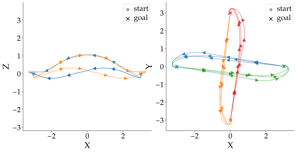
Evaluation measures throughput, success, objective value, iteration counts and deviation from IPOPT. All experiments use double precision, a convergence tolerance of 10⁻⁸ and a 500-iteration limit on one 48 GB NVIDIA L40S and a 64-core, dual-socket AMD EPYC 9354 host. Three quadrotor benchmarks probe heterogeneous difficulty, tracking difficulty and problem dimension; no physical-robot deployment is reported.
VI-A Experimental Setup
The quadrotor model has 13 state coordinates and four rotor inputs. A 0.1-second step and 30-step horizon yield at least 506 optimization variables per vehicle before inequality slacks. IPOPT-default solves one problem at a time with a multithreaded linear solver; IPOPT-64 runs 64 independent single-core instances. MadNLP accelerates sequential solves on the GPU. The jaxipm-noIL ablation disables iteration-level replacement. Every method receives the same parameter/initialization pool, containing four times the selected GPU batch size.
| Solver | solves/s | equiv. instances | success (%) | cost | iters mean/max |
| IPOPT-default | 6.99 0.28 | 1.00 | 100 | 507.6 17.1 | 21.5 / 71 |
| IPOPT-64 | 310.9 14.8 | 44.5 | 100 | 507.6 17.1 | 21.5 / 71 |
| MadNLP | 2.74 0.02 | 0.39 | 100 | 507.6 17.2 | 32.2 / 184 |
| jaxipm-noIL | 14.08 1.12 | 2.01 | 99.55 | 507.6 17.2 | 71.6 / 468 |
| jaxipm | 95.45 1.24 | 13.7 | 100 | 507.6 16.5 | 51.9 / 252 |
VI-B What throughput does jaxipm achieve?
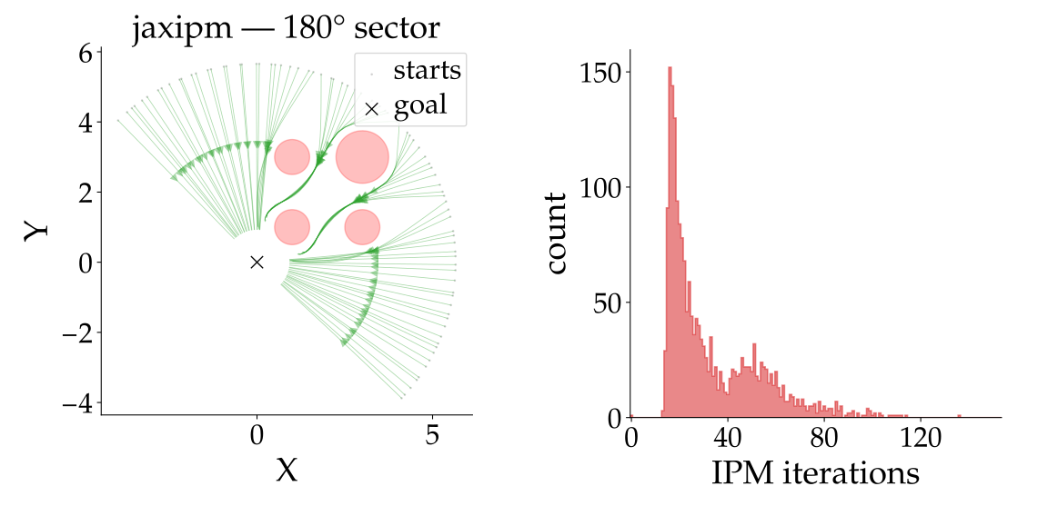
Navigation starts lie along a 180° arc around a common goal with obstacles, producing widely different solve lengths. With batch size 500, jaxipm reaches 95.45 solves/s versus 6.99 for IPOPT-default, 2.74 for MadNLP and 310.9 for IPOPT-64. That is 13.7× the sequential CPU baseline and 30.7% of the parallel CPU baseline. Removing iteration-level replacement drops throughput to 14.08 solves/s, about 14.8% of the full method. Costs are comparable; full jaxipm succeeds on all tested instances.
VI-C How does problem difficulty affect jaxipm ?
Tracking a periodic reference among known moving obstacles uses batch size 250; increasing reference speed raises difficulty. jaxipm achieves 15.3–28.9× IPOPT-default throughput and 39.4–69.9% of IPOPT-64 throughput. Its batch linear solver cannot reliably perform iterative refinement, so less accurate steps affect easy problems disproportionately and sometimes reach different local minima. Without slot replacement, success falls to 86.1% at the highest speed. The authors attribute this to converged, ill-conditioned systems remaining in the batch and affecting other linear solves; replacement removes them. The full variant reports 100% success in these tests, not a general robustness guarantee.
| Solver | solves/s | equiv. instances | success (%) | cost | iters mean/max |
| m/s | |||||
| IPOPT-default | 6.06 0.30 | 1.00 | 100 | 265.7 98.7 | 25.4 / 77 |
| IPOPT-64 | 234.7 9.5 | 38.7 | 100 | 265.7 98.7 | 25.4 / 77 |
| MadNLP | 2.97 0.99 | 0.49 | 100 | 261.7 92.0 | 38.0 / 84 |
| jaxipm-noIL | 13.00 0.71 | 2.15 | 99.2 | 249.8 79.4 | 54.2 / 472 |
| jaxipm | 92.49 0.37 | 15.3 | 100 | 244.0 76.3 | 43.1 / 181 |
| m/s | |||||
| IPOPT-default | 4.61 0.27 | 1.00 | 100 | 556.7 140.9 | 30.3 / 71 |
| IPOPT-64 | 185.4 3.8 | 40.2 | 100 | 556.7 140.9 | 30.3 / 71 |
| MadNLP | 2.02 0.01 | 0.44 | 100 | 555.8 138.3 | 47.4 / 116 |
| jaxipm-noIL | 11.85 0.07 | 2.57 | 96.2 | 543.2 126.5 | 54.3 / 494 |
| jaxipm | 81.76 0.37 | 17.7 | 100 | 539.2 121.4 | 44.4 / 237 |
| m/s | |||||
| IPOPT-default | 2.55 0.14 | 1.00 | 100 | 1146.7 126.9 | 47.8 / 125 |
| IPOPT-64 | 105.4 3.7 | 41.3 | 100 | 1146.7 126.9 | 47.8 / 125 |
| MadNLP | 1.65 0.00 | 0.65 | 100 | 1147.5 121.2 | 57.8 / 136 |
| jaxipm-noIL | 11.32 0.22 | 4.44 | 86.1 | 1140.5 125.3 | 46.9 / 165 |
| jaxipm | 73.71 0.87 | 28.9 | 100 | 1142.4 131.5 | 45.8 / 129 |
VI-D How does dimensionality affect jaxipm ?
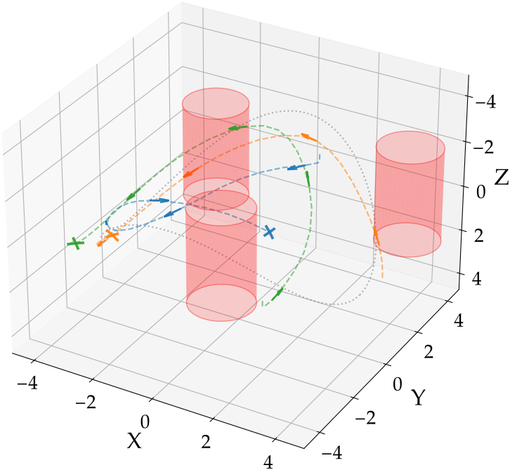
Two or four quadrotors swap positions while maintaining pairwise separation, giving 1,012 or 2,024 variables and batch size 75. jaxipm achieves 18.42 and 4.54 solves/s respectively, equivalent to 31.9 and 15.7 sequential IPOPT instances, or 69.8% and 32.5% of IPOPT-64 throughput. Larger problems reduce the useful batch size within GPU memory. Iteration replacement helps less for these relatively homogeneous initial conditions, though the four-vehicle ablation succeeds on 95% versus 100% for the full method. Four-vehicle costs and iteration counts also differ from IPOPT, consistent with the linear-solve limitations.
| Solver | solves/s | equiv. instances | success (%) | cost | iters mean/max |
| 2 quadrotors | |||||
| IPOPT-default | 0.578 0.018 | 1.00 | 100 | 755.5 0.8 | 112.6 / 135 |
| IPOPT-64 | 26.38 0.98 | 45.6 | 100 | 755.5 0.8 | 112.7 / 135 |
| MadNLP | 1.07 0.14 | 1.84 | 100 | 755.5 0.8 | 127.7 / 162 |
| jaxipm-noIL | 17.31 0.46 | 29.9 | 100 | 755.5 0.8 | 115.7 / 176 |
| jaxipm | 18.42 0.20 | 31.9 | 100 | 755.5 0.8 | 113.6 / 182 |
| 4 quadrotors | |||||
| IPOPT-default | 0.289 0.008 | 1.00 | 100 | 1529.7 4.7 | 95.5 / 159 |
| IPOPT-64 | 13.99 0.13 | 48.4 | 100 | 1529.7 4.7 | 93.3 / 140 |
| MadNLP | 0.596 0.008 | 2.06 | 100 | 1529.7 4.7 | 184.1 / 217 |
| jaxipm-noIL | 2.62 0.03 | 9.06 | 95 | 1533.9 8.3 | 241.7 / 498 |
| jaxipm | 4.54 0.05 | 15.7 | 100 | 1533.7 8.9 | 227.3 / 484 |
VI-E Does jaxipm produce the same results as IPOPT?
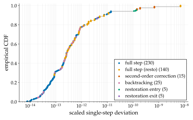
The parity experiment saves each complete IPOPT state on difficult navigation solves, loads that state into jaxipm, executes one step and compares with IPOPT’s next state using the scaled maximum difference in Equation 4. All measured deviations across five optimizations are below 10⁻⁸, including activated restoration, correction and barrier-update branches. This is a state-reinitialized one-step comparison with conservative single-instance iterative refinement. It does not establish identical uninterrupted batched trajectories or cover every possible branch/problem; reliable iterative refinement is explicitly unavailable in the reported batch setting.
Equation 4
| (4) |
VII Conclusion
The contribution is a GPU-batched reconstruction of a robust nonlinear solver, with high throughput from branch fusion and prompt replacement of finished instances. The experiments support benefits over sequential IPOPT and MadNLP but show a remaining gap to 64 parallel CPU instances. GPU memory, inner-loop synchronization and batch linear-solve accuracy constrain performance. Generating trajectory datasets and embedding constrained optimization within sampling-based learning/control are proposed applications rather than demonstrated downstream results.