Overview
Project website. This edition follows the complete twenty-seven-page v2 of 24 September 2026. All twelve numbered figures, including six native subplot graphics absent as ordinary images in the HTML, ten numbered tables and fifteen displayed equations are retained. The online controller uses RGB; building each garment’s simulator asset requires an offline RGB-D capture.
At a glance
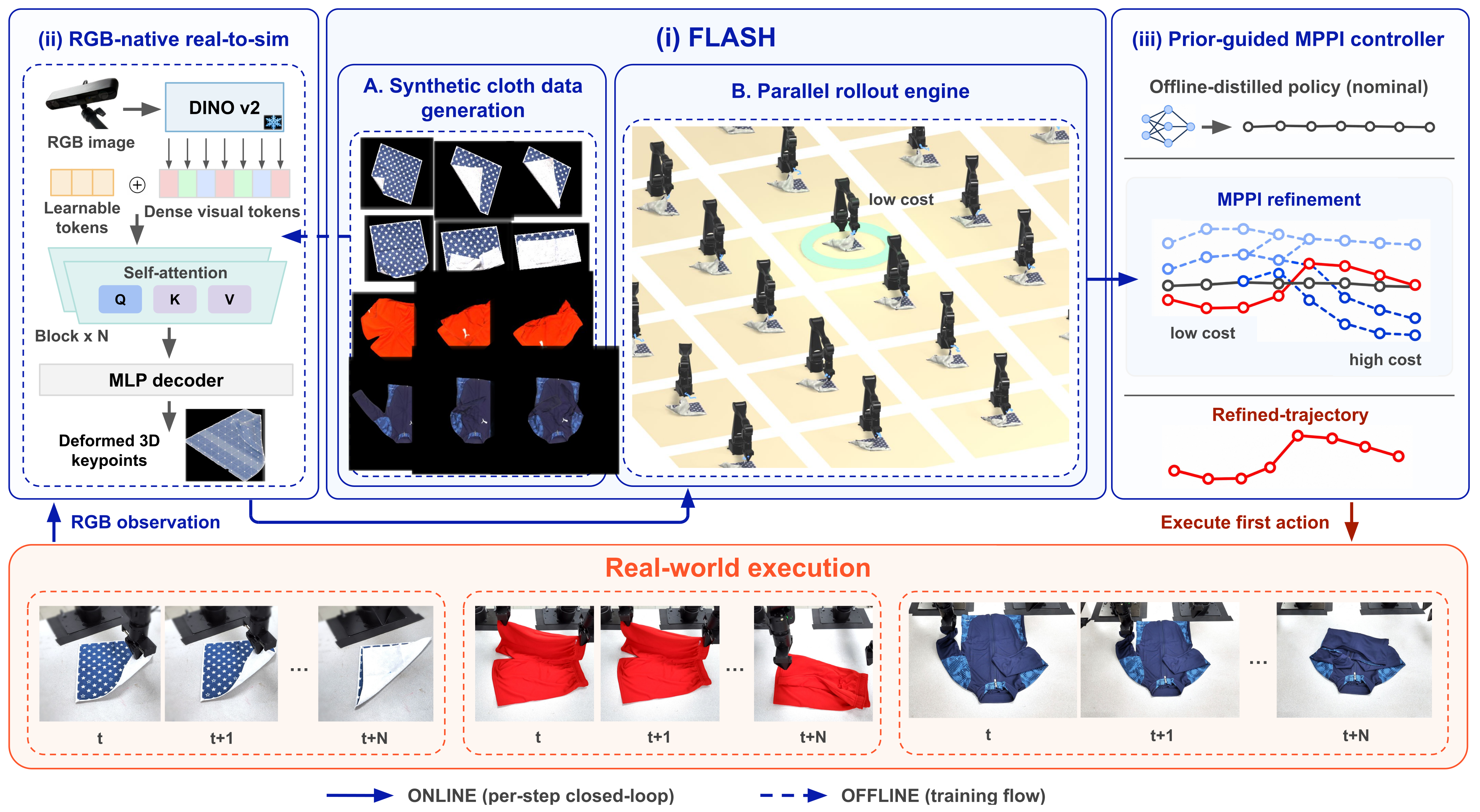
A learned cloth policy proposes a short action sequence, then a physical simulator evaluates nearby alternatives before the robot executes the first refined action. A single RGB image predicts the current garment mesh, resetting simulation at every control cycle. FLASH supplies parallel contact-rich rollouts; prior-guided model predictive path integral control (MPPI) turns their costs into an action update.
In ten-trial towel experiments, full-system success is 9/10 with one arm and 8/10 with two, compared with 3/10 and 1/10 for the base policy. Additional garment, task and disturbance tests support this approach within calibrated, quasi-static tabletop folding. New garments receive separate assets, estimator training and prior policies; these are not zero-shot garment transfers.
1 Introduction
Cloth state is high-dimensional and partly hidden, while contact, friction and folding make long-horizon prediction sensitive to errors. Learned policies can miss unusual states; uncontrolled simulator rollout can drift away from reality. This system joins learned proposals with short physical look-ahead and repeated visual state correction.
The intended contribution is a practical loop built from FLASH, fixed-correspondence mesh estimation and MPPI. It does not learn a new dynamics model. The experiments examine each component and complete folding performance rather than establish a general robustness guarantee.
2 Related Works
Prior cloth manipulation includes reinforcement/imitation learning, semantic keypoints, learned dynamics and feedback-based trajectory adaptation. MeshGraphNets and AdaptiGraph learn dynamics, whereas this work uses an explicit physical simulator at inference. AdaFold and other feedback approaches motivate correcting rather than blindly replaying a trajectory.
State reconstruction relates to TRTM, Cloth-Splatting and UniClothDiff’s generative state estimation. Here the estimator predicts an asset’s indexed mesh vertices directly from RGB. Sampling-based planning avoids differentiating contact dynamics, while the learned prior narrows the search around plausible folds.
3 Method
The method combines a reusable physical rollout engine, garment-specific RGB reconstruction and prior-guided sampling control. The preserved equations distinguish visual mesh prediction from the full position-and-velocity state needed by simulation.
3.1 System Overview
At each cycle, an RGB frame predicts vertex positions, the simulator is synchronized, and the base policy generates a nominal action sequence. MPPI perturbs that sequence, simulates the candidates and averages them using cost-dependent weights. Only the first refined action is executed before observing again.
The simulator state contains positions and velocities, but a single frame estimates only positions. Velocities are reset to zero. That is a quasi-static modeling assumption, not a consequence that zero is the only possible physical velocity consistent with one image; motion would require temporal information or another prior.
Equations 1–2
| (1) |
| (2) |
3.2 Simulator Backbone
FLASH represents cloth as a triangular mesh with finite-element stretching, isometric bending and Signorini–Coulomb contact/friction. Its GPU implementation combines local–global iterations with a nonsmooth Newton contact solve, allowing many short rollouts in parallel.
Physical contact and global deformation structure distinguish it from learned forward prediction, while repeated visual resets limit accumulated state drift. Material parameters and grasp/contact approximations still affect candidate ranking; resetting state does not remove these modeling errors.
Equation 3
| (3) |
3.3 RGB-native Real-to-Sim Reconstruction
Each garment has a fixed mesh topology and ordered canonical vertices. The network estimates all corresponding 3D positions, including occluded regions, so its output can directly initialize the simulator. This correspondence is learned for that asset rather than recovered for arbitrary unseen garments.
Equation 4
| (4) |
Simulator asset construction.
One overhead RGB-D capture supplies the rest mesh: SAM 2 segments the garment, depth is back-projected, ball-pivoting forms a surface, and remeshing/smoothing regularizes it while preserving the boundary. Depth is used in this offline construction, although the deployed estimator consumes RGB alone.
Synthetic supervision.
FLASH generates paired rendered RGB images and ground-truth vertex positions from randomized scripted folds and additional gravity-settled states. Camera calibration aligns these samples with the fixed real viewpoint. Simulation supervision avoids manually labeling full real cloth meshes.
Equation 5
| (5) |
Network architecture.
A frozen DINOv2 backbone produces visual patch features. A trainable projection maps them to the canonical-token dimension; four self-attention blocks jointly process image tokens and one learned token per mesh vertex. A shared decoder maps each updated canonical token to its 3D position.
Canonical indices preserve vertex correspondence across deformations. The network uses global image context to infer hidden geometry, but occluded positions remain predictions conditioned on training distribution rather than directly observed ground truth.
Equations 6–8
| (6) |
| (7) |
| (8) |
Training objective.
Training minimizes smooth-L1 error between predicted and simulated vertex positions. The visual backbone stays frozen; the projection, canonical tokens, attention blocks and decoder are optimized. This supervised objective does not explicitly enforce every physical constraint of the reconstructed mesh.
Equation 9
| (9) |
Robust augmentation.
Color, illumination, blur, grayscale, erasing and grasp-centered occlusion randomization reduce reliance on simulator appearance and visible grippers. Token masking additionally removes overlapping visual patches during some occlusion augmentations. Appendix D tests the combined augmentation package rather than identifying each component’s separate effect.
3.4 Prior-Guided MPPI Refinement
The nominal sequence comes from a garment-specific MLP prior trained by on-policy imitation of a scripted teacher in FLASH. It supplies a plausible local search center; inference-time refinement adjusts its action choices using the reconstructed state.
Prior-guided online refinement.
Independent Gaussian perturbations produce candidate sequences around the prior. Every candidate starts from the same reconstructed positions and zero velocities, rolls out through the simulator and receives a task/constraint cost. Exponentiated negative costs are normalized, and their weights average the candidate actions.
Deployment uses 256 candidates, a five-action horizon, 5 mm noise scale and temperature 0.08. Costs reward reaching/folding and penalize table/workspace violations, action magnitude and fold-height error. These are soft penalties, not certified hard constraints; the weighted action average is a sampled optimization update rather than proof of optimality or safety.
Equations 10–13
| (10) |
| (11) |

Original selectable MathML
| (12) |
| (13) |
Receding-horizon execution.
Only the first action of the refined sequence is sent to the robot. A new RGB observation then overwrites simulated positions and the process repeats. This closes the loop around model errors and disturbances, within the estimator’s and controller’s operating range.
4 Experiments
The evaluation separates simulator performance, synthetic mesh reconstruction, end-to-end towel folding and selected extensions. The hardware comparisons use ten trials per setting and report descriptive success rates without uncertainty intervals or significance tests.
4.1 Simulator Backbone
Baselines.
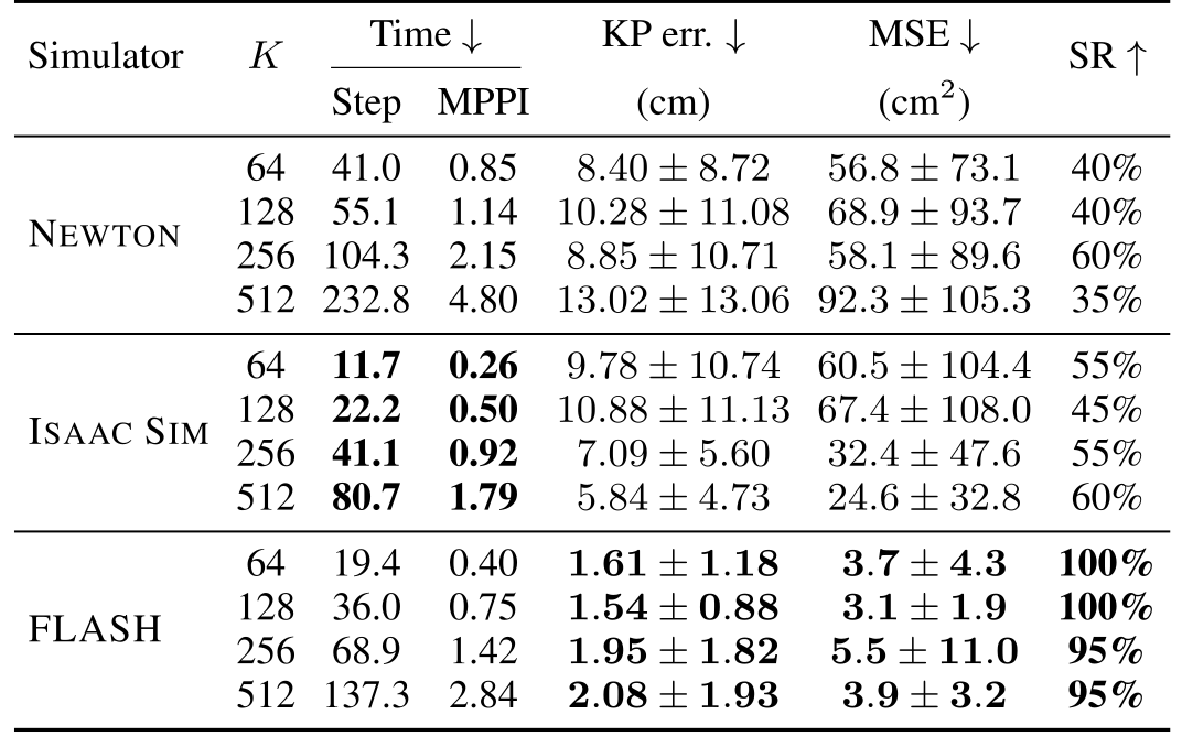
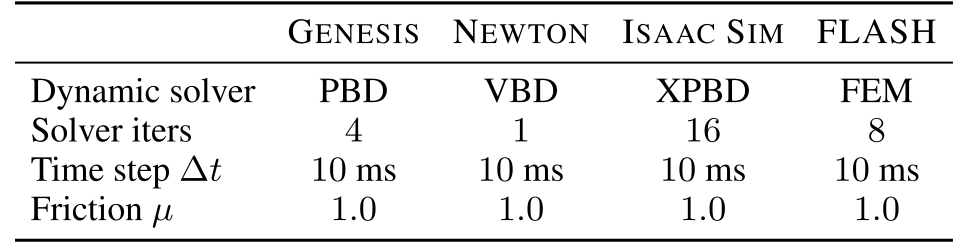
The same vanilla MPPI towel-folding protocol compares FLASH with Genesis, Newton and Isaac Sim. Genesis develops unstable dragging/folding behavior and fails all tested settings, so the numerical table covers the other three. These are configured implementations with different models, particle counts and solver parameters, not materially matched engines.
Original selectable table
| Simulator | Time | KP err. | MSE | SR | ||
| Step | MPPI | (cm) | (cm2) | |||
| Newton | 64 | 41.0 | 0.85 | 40% | ||
| 128 | 55.1 | 1.14 | 40% | |||
| 256 | 104.3 | 2.15 | 60% | |||
| 512 | 232.8 | 4.80 | 35% | |||
| Isaac Sim | 64 | 11.7 | 0.26 | 55% | ||
| 128 | 22.2 | 0.50 | 45% | |||
| 256 | 41.1 | 0.92 | 55% | |||
| 512 | 80.7 | 1.79 | 60% | |||
| FLASH | 64 | 19.4 | 0.40 | 100% | ||
| 128 | 36.0 | 0.75 | 100% | |||
| 256 | 68.9 | 1.42 | 95% | |||
| 512 | 137.3 | 2.84 | 95% | |||
Metrics.
Twenty shared initializations per sampling budget vary towel pose. Success requires keypoint error below 5 cm; final mesh, Chamfer and earth mover distances assess fold shape separately. The mesh MSE uses the moved half’s 231 vertices against mirrored target partners, rather than every mesh vertex against a measured real cloth state. Step time and full MPPI time capture different compute costs.
Results.
Across 64/128/256/512 samples, FLASH succeeds in 100/100/95/95% of trials, with keypoint errors of 1.61/1.54/1.95/2.08 cm. Isaac Sim is about 1.7 times faster per step but reaches only 45–60% success; Newton reaches 35–60%. FLASH’s full MPPI time rises from 0.40 to 2.84 s as samples increase.
These in-simulator folding results favor the selected FLASH configuration, not a universal engine ranking or a direct measurement of physical fidelity. Appendix C separately replays real trajectories to assess agreement with observed cloth geometry.
4.2 State Estimation
Baselines.
DPM adapts UniClothDiff’s point-cloud diffusion estimator to the same garment assets and single overhead view. The DeFM baseline replaces RGB features with a frozen depth backbone and the same canonical reconstruction head. The comparison changes representation/backbone as well as modality, so it is not a pure causal RGB-versus-depth test.
Metrics.
Synthetic held-out episodes provide ground-truth vertex MSE, Chamfer distance and earth mover distance, with inference latency measured on the same GPU. These metrics have different units: MSE is in mm² and the two point-set distances are in mm.
Results.
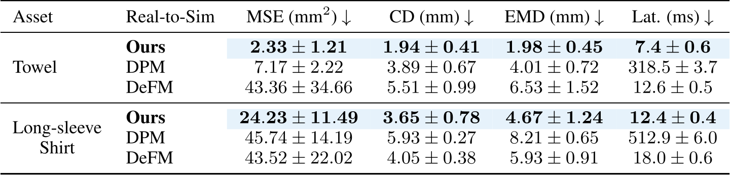
For towels, the RGB estimator achieves 2.33 mm² MSE, 1.94 mm Chamfer distance and 7.4 ms latency, versus DPM’s 7.17 mm², 3.89 mm and 318.5 ms. For shirts, its corresponding values are 24.23 mm², 3.65 mm and 12.4 ms; DeFM has 43.52 mm², 4.05 mm and 18 ms.
These are synthetic-validation results from the authors’ reproduced baselines. Real observations have larger error in Appendix C, and the adapted DPM protocol differs from UniClothDiff’s original multi-view setting.
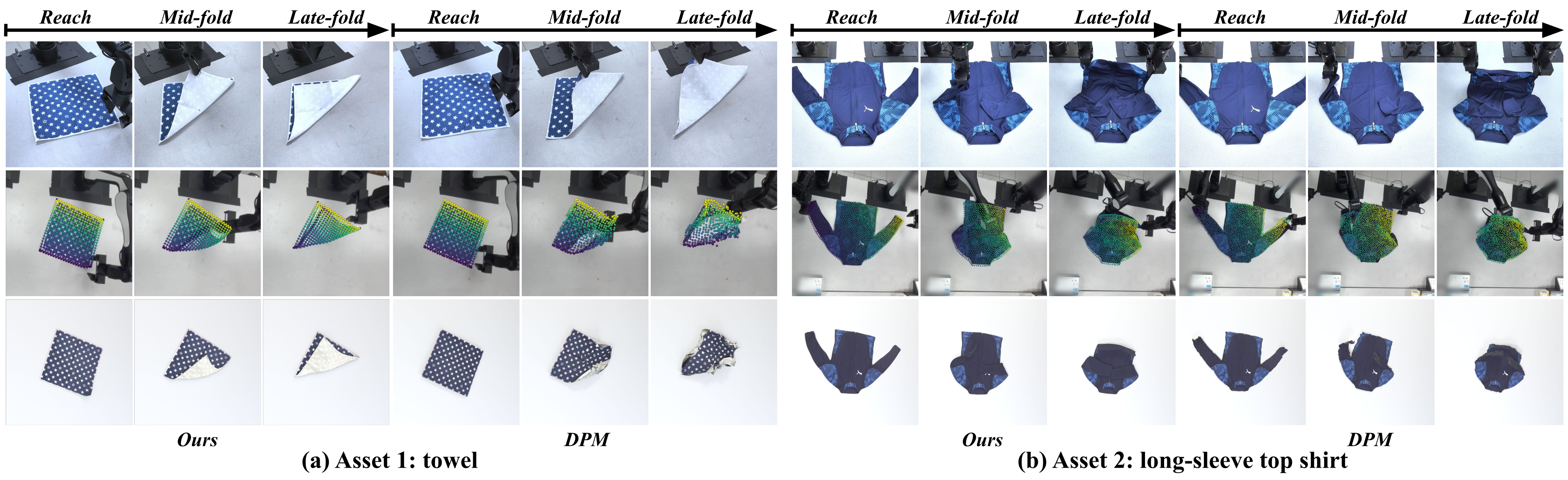
4.3 Real-World Evaluation
Tasks.
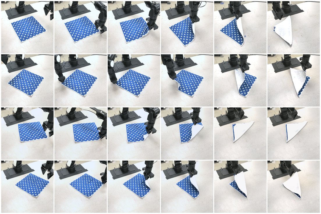
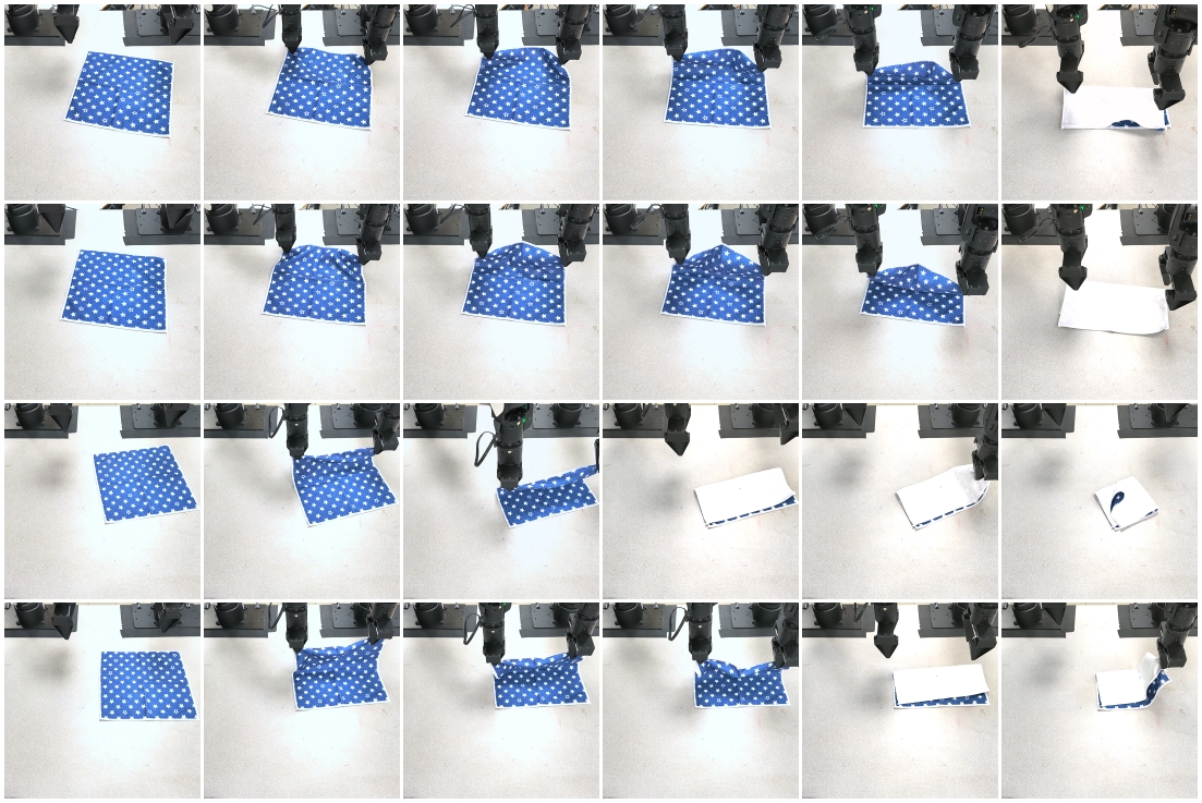
Single- and dual-arm AIRBOT Play systems fold a square towel from randomized initial states using a fixed overhead camera. Each of ten trials includes reaching, grasping and folding. Success requires all necessary grasps and all target corner pairs within 2 cm; failed grasps are not removed or rerun.
Baselines.
Component substitutions replace the RGB estimator with DPM or FLASH with Isaac Sim while retaining the surrounding system. A base-policy condition omits online refinement. The tests show contributions under the selected setup, not that each design is universally necessary.
Results.
Single-arm successes are 9/10 for the full method, 6/10 with DPM, 5/10 with Isaac Sim and 3/10 for the prior alone. Dual-arm results are 8/10, 3/10, 4/10 and 1/10. Full-system grasping succeeds in all single-arm trials and nine dual-arm trials; folding can still fail after a successful grasp.
Towel-cycle compute is about 1.075 s: segmentation 95.8 ms, reconstruction 8.5 ms, state transfer 0.5 ms and MPPI 970 ms. Actuation adds time. The loop therefore supports slow manipulation rather than high-frequency control; MPPI alone takes 2.55 s for the larger shorts mesh.
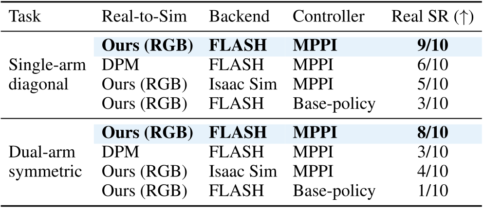
Original selectable table
| Task | Real-to-Sim | Backend | Controller | Real SR () |
| Single-arm diagonal | Ours (RGB) | FLASH | MPPI | 9/10 |
| DPM | FLASH | MPPI | 6/10 | |
| Ours (RGB) | Isaac Sim | MPPI | 5/10 | |
| Ours (RGB) | FLASH | Base-policy | 3/10 | |
| Dual-arm symmetric | Ours (RGB) | FLASH | MPPI | 8/10 |
| DPM | FLASH | MPPI | 3/10 | |
| Ours (RGB) | Isaac Sim | MPPI | 4/10 | |
| Ours (RGB) | FLASH | Base-policy | 1/10 |
4.4 Generalization and Closed-Loop Correction
Tasks.
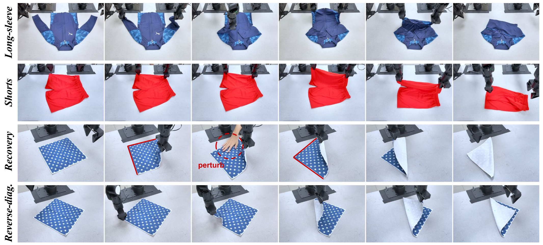
Extensions fold shirts and shorts, reverse the towel diagonal and recover from a human push during folding. New garments require their own mesh, synthetic data, estimator, material tuning and prior policy. The shared element is the simulator/control framework. Reversing the towel diagonal instead changes goal keypoints without retraining the towel prior.
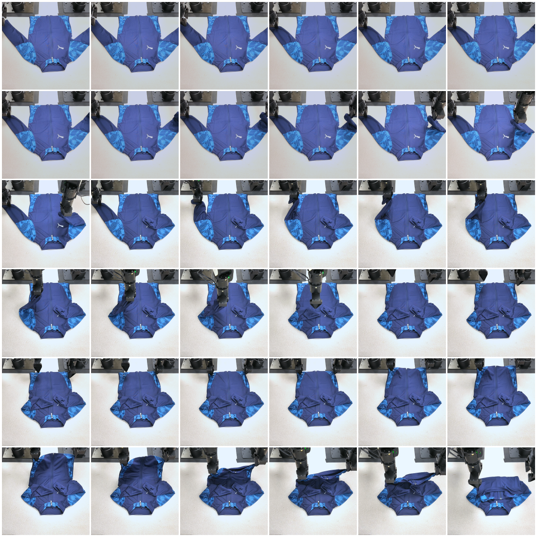
Shirts fold sleeves inward and then the torso; shorts fold legs toward the waistband and then compact the garment. Trials randomize initial translations by up to 5 cm and yaw by 0.5 rad. Human perturbation amplitude is not quantified by this hardware experiment.
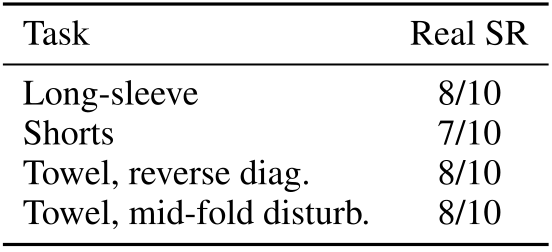
Original selectable table
| Task | Real SR |
| Long-sleeve | 8/10 |
| Shorts | 7/10 |
| Towel, reverse diag. | 8/10 |
| Towel, mid-fold disturb. | 8/10 |
Results.
Ten trials per condition yield 8/10 shirt folds, 7/10 shorts folds, 8/10 reversed-diagonal folds and 8/10 disturbance recoveries. Successful examples show adaptation beyond the original towel trajectory, but the small samples and per-garment preparation limit claims of generalization.
5 Conclusion
Repeated RGB reconstruction and physical look-ahead improve the studied cloth-folding policies, with gains from both the simulator and estimator in component comparisons. The practical result is a calibrated simulator-in-the-loop method for selected garments and slow tasks, with explicit preparation and compute costs.
6 Limitations and Future Work
Limits include per-garment training and parameter tuning, a fixed overhead viewpoint, imperfect simulator fidelity and substantial rollout cost. Tested garments are woven textiles of comparable thickness; thick or qualitatively different materials and fast motion are not established capabilities. Broader visual reconstruction and faster rollout engines are future directions.
Acknowledgments
The acknowledgments identify supporting institutions and funding; the technical and empirical claims are those of the paper.
Appendix
A Implementation Details
Appendix A specifies the asset pipeline, network, randomization, controller costs and modeling assumptions needed to reproduce the loop.
A.1 RGB-native Real-to-Sim Reconstruction
A 392×392 image yields 784 frozen DINOv2-S/14 patch features of dimension 384, projected to 256. The towel, shorts and shirt meshes have 464, 1,156 and 1,379 vertices. Four pre-normalized attention blocks use eight heads and dropout 0.1; a shared layer-normalization/two-hidden-layer GELU decoder outputs coordinates.
Canonical tokens start from deterministic Gaussian Fourier features of rest coordinates, with frequency scale 4. The Fourier matrix is fixed while tokens themselves are learnable. Synthetic examples include randomized scripted folds and gravity-settled meshes. Train/validation splitting is 90/10 by episode to avoid nearby frames leaking across the split.
Training uses AdamW, learning rate 3×10⁻⁴, weight decay 10⁻⁴, gradient clipping at 1, batch size 32 and fifty epochs; cosine decay follows three warmup epochs, with EMA 0.999. Grasp occlusion occurs with probability 0.7; token masking probability 0.8 is conditional on that augmentation, not an independent 80% mask of all inputs. Table A1 preserves the complete appearance/occlusion settings.
Preparing a new asset requires roughly one hour of synthetic generation and twelve hours of estimator training on an RTX 4090, in addition to capture/meshing. Thus asset-specific synthetic supervision remains a significant adaptation cost.
Equations 14–15
| (14) |
| (15) |
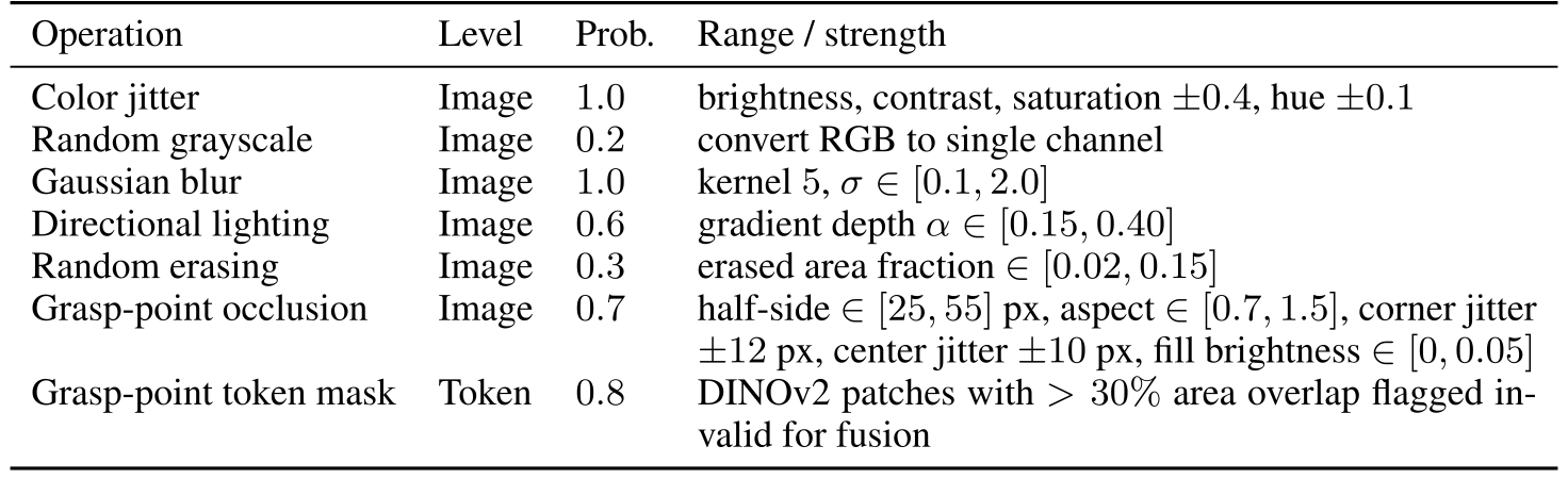
Original selectable table
| Operation | Level | Prob. | Range / strength |
| Color jitter | Image | brightness, contrast, saturation , hue | |
| Random grayscale | Image | convert RGB to single channel | |
| Gaussian blur | Image | kernel , | |
| Directional lighting | Image | gradient depth | |
| Random erasing | Image | erased area fraction | |
| Grasp-point occlusion | Image | half-side px, aspect , corner jitter px, center jitter px, fill brightness | |
| Grasp-point token mask | Token | DINOv2 patches with area overlap flagged invalid for fusion |
A.2 Prior-Guided MPPI Control
The prior is a 512/256/128 MLP taking sparse mesh features and predicting end-effector actions. MPPI rolls it forward to obtain the nominal horizon before adding noise. Table A2 retains all phase-dependent cost expressions and weights.
Reaching uses 3D pick-point distance; folding uses in-plane corner-to-goal distance, with matching terminal costs. Squared hinge penalties discourage table penetration and workspace violations, and fold-height error is squared. The term described as action smoothness penalizes action magnitude, not differences between consecutive actions. Table/workspace margins are 5 mm and 2 cm.
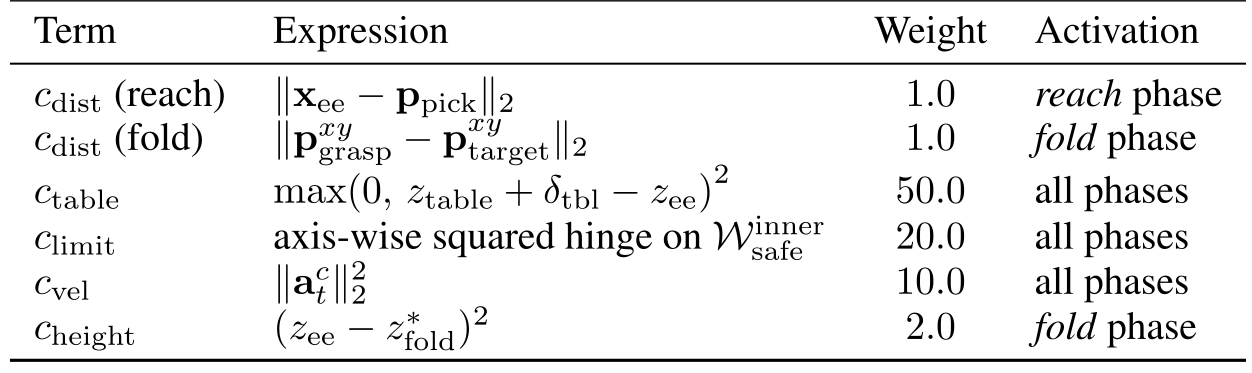
Original selectable table
| Term | Expression | Weight | Activation |
| (reach) | reach phase | ||
| (fold) | fold phase | ||
| all phases | |||
| axis-wise squared hinge on | all phases | ||
| all phases | |||
| fold phase |
A.3 Modeling Assumptions
The gripper is a rigid box that pins selected garment vertices after grasping; finger slip, partial grasp and regrasp dynamics are not modeled. Garment mass, bending and friction are tuned individually. Position resets correct accumulated state drift but cannot make these assumptions exact.
Zeroing velocity restricts the intended regime to quasi-static actions. A proposed RGB-D frontend for broader materials is a future extension, not evidence that the current RGB estimator or tested parameters already handle them.
B Experiment Details
Appendix B fixes the simulator, estimator and robot evaluation protocols and retains the full visual folding sequences.
B.1 Simulator Backbone Comparison
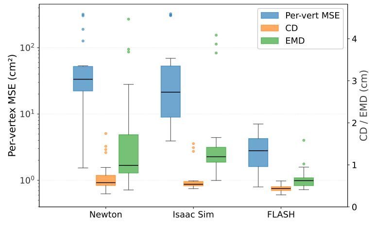
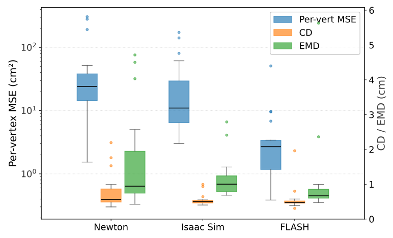
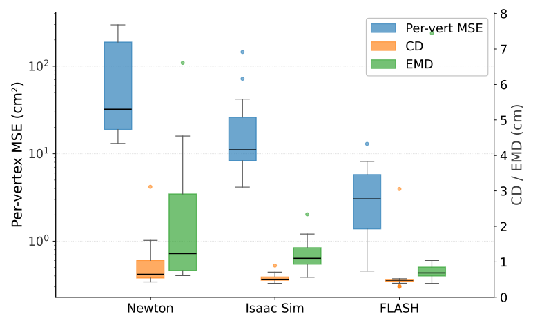
The simulator benchmark uses a 30×30 cm, 464-vertex towel, vanilla MPPI with horizon six, 40 ms action steps and four 10 ms physics steps per action. End-effector increments are clamped to 20 mm. Twenty shared seeds randomize initial translation by up to 8 cm and yaw by 30°. After keypoint error falls below 5 cm, another 150 settling steps precede final shape scoring.
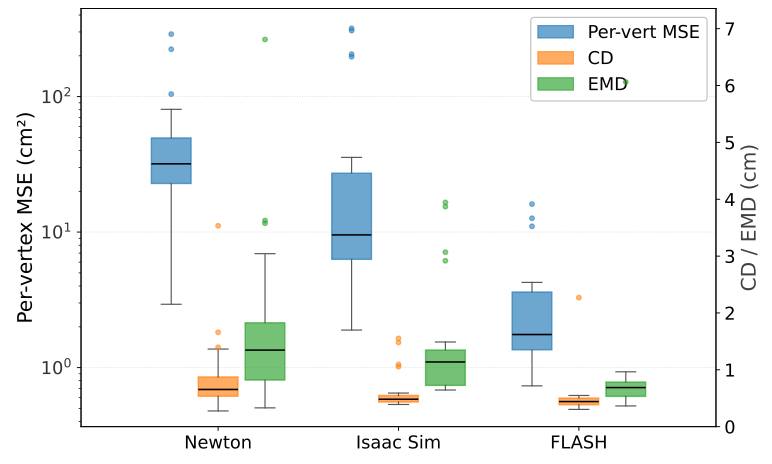
All engines use friction one, but their other parameters differ substantially: Genesis uses PBD and more internal particles; Newton uses one VBD iteration; Isaac uses sixteen XPBD iterations; FLASH uses FEM with eight local–global and ten constraint iterations. Different stiffness, mass/density and solver choices prevent interpreting Table 1 as a matched-material physics experiment. Figure B1 retains all four distribution plots.
B.2 State Estimation
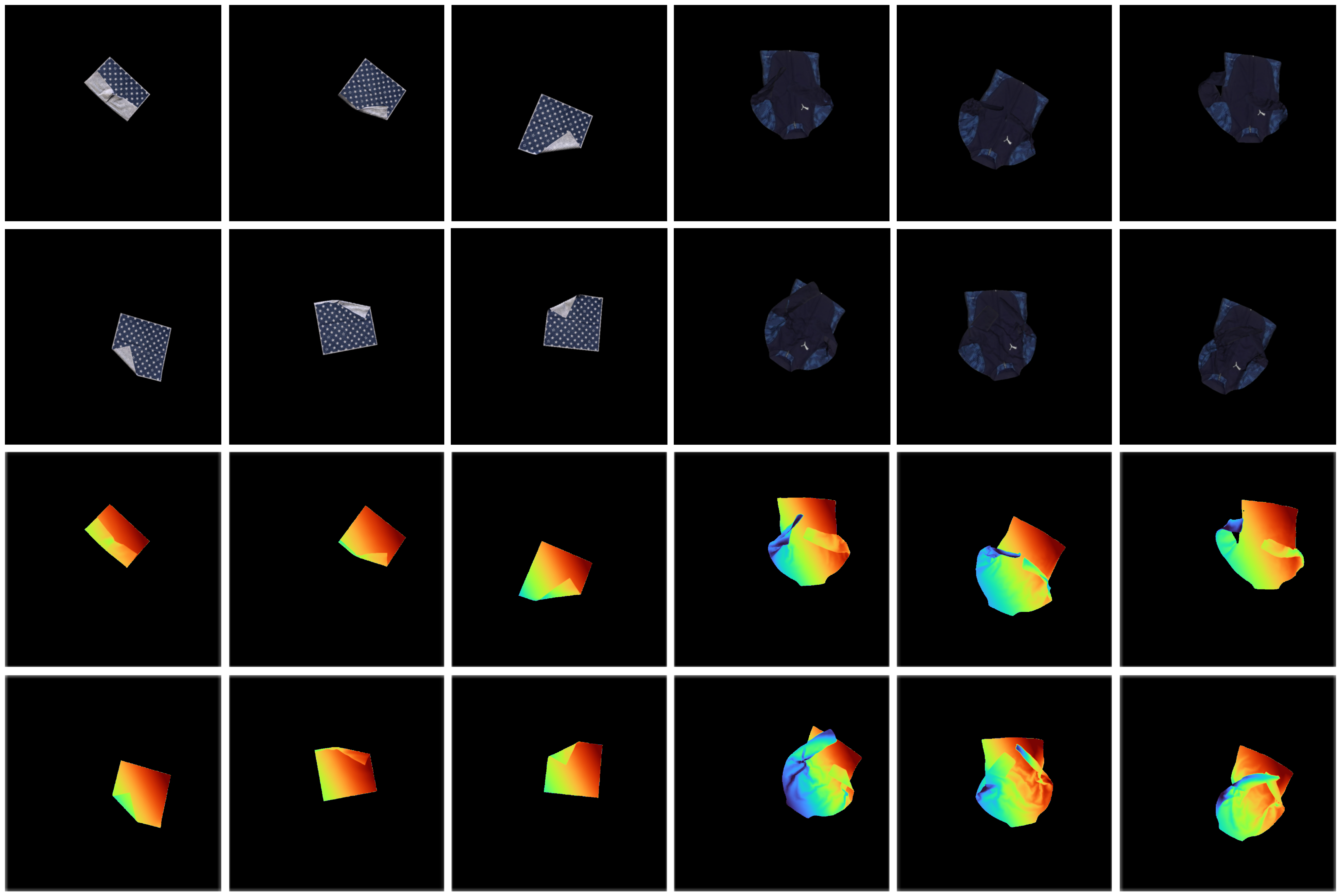
The estimator test shares garment topology, simulated fold distributions and episode-based held-out data. Table B2 specifies the architectures, inputs and training settings. Figure B2 shows synthetic RGB/depth examples of towel and shirt folds and rest states.
DPM consumes 10,000 points from the single overhead depth cloud. DeFM uses a frozen depth encoder with the same canonical head and supervision as the RGB system. Matching these downstream components narrows the comparison while leaving differences in pretraining and representations.
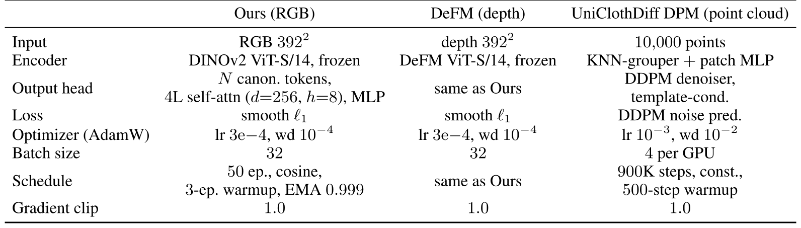
Original selectable table
| Ours (RGB) | DeFM (depth) | UniClothDiff DPM (point cloud) | |
| Input | RGB | depth | points |
| Encoder | DINOv2 ViT-S/14, frozen | DeFM ViT-S/14, frozen | KNN-grouper patch MLP |
| Output head | canon. tokens, L self-attn (, ), MLP | same as Ours | DDPM denoiser, template-cond. |
| Loss | smooth | smooth | DDPM noise pred. |
| Optimizer (AdamW) | lr , wd | lr , wd | lr , wd |
| Batch size | per GPU | ||
| Schedule | ep., cosine, -ep. warmup, EMA | same as Ours | K steps, const., -step warmup |
| Gradient clip |
B.3 Real-World Evaluation
The hardware uses one or two six-degree-of-freedom arms with binary parallel grippers and synchronized end-effector position increments. The ZED 2i supplies 1280×720 overhead images; the RGB method uses the left color view, while depth supports its baseline and separate evaluation.
The complete trial includes all phases, with the same end-to-end success rule and ten initializations per condition. Runtime measurements report perception, state transfer and rollout separately. Success after grasping remains stricter than successful grasp acquisition alone.
Visualizations.
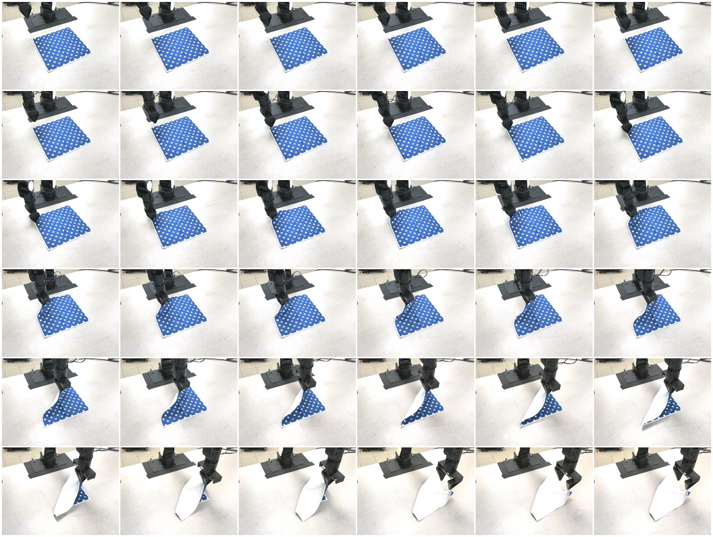
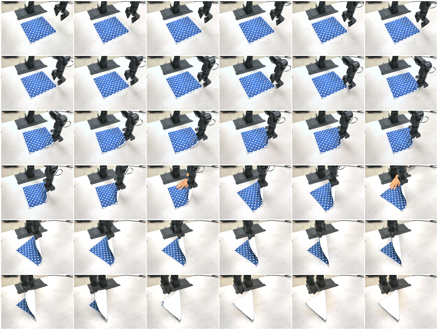
Figures B3 and B4 preserve full single- and dual-arm towel sequences. They illustrate the observed reach–grasp–fold process; quantitative rates come from the full trial sets rather than these selected examples.
B.4 Generalization and Closed-Loop Correction
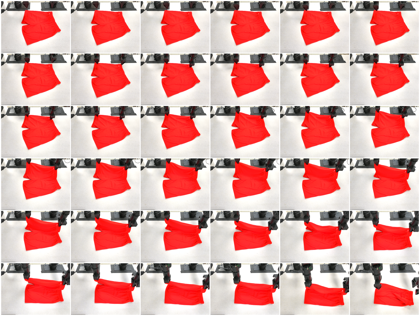
Figures B5–B8 retain shirt folding, shorts folding, reversed-diagonal towel folding and recovery after a mid-fold disturbance. Garment-specific estimator/prior training and tuned physical parameters accompany shirt/shorts transfer. Reversed-diagonal towel folding reuses the learned prior with altered goals.
The disturbance example shows successive visual resets recovering useful actions. Its qualitative human push should not be assigned the precisely controlled 6/9/12 cm amplitudes used in the separate simulation analysis.
C Additional Experimental Analyses
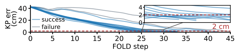
C.1 Simulator Fidelity Against Real Cloth Trajectories
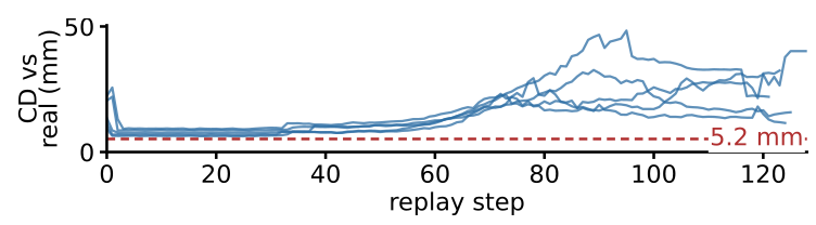
Five recorded real trajectories contain 626 frames. The simulator receives the initial mesh once, then replays measured robot motion without visual resets. A one-sided nearest-neighbor Chamfer distance from simulated vertices to recorded depth points has median 13.6 mm, typically 7–9 mm early and larger during dragging.
Flat-cloth registration has a 5.2 mm measurement floor combining camera, segmentation and mesh alignment. This cannot simply be subtracted to isolate physical-model error. The one-sided metric also does not establish material-point correspondence or complete agreement on hidden surfaces. Figure C1 retains both replay and disturbance plots.
C.2 State-Estimation Error on Real Observations
On the same five real trajectories, RGB mesh estimates have 10.2±1.4 mm mean per-trajectory distance to the observed depth cloud. Depth measures error here rather than serving as estimator input. The value exceeds synthetic validation errors and is not directly interchangeable with the simulator replay’s median 13.6 mm: aggregation and evaluated states differ.
C.3 Closed-Loop Error Trajectories and Disturbance Magnitude
Twenty simulated folding seeds yield eighteen successes below the 2 cm criterion, ending at 0.8±0.1 cm after 22–31 steps. The initial 42.2 cm is the approximately full towel diagonal in the task’s keypoint error, not a 42.2 cm reconstruction error.
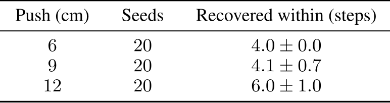
Controlled 6/9/12 cm pushes eight steps after motion begins require 4±0, 4.1±0.7 and 6±1 steps respectively to return below the pre-disturbance error, over twenty seeds each. This recovery measure is not time to finish folding and does not establish a formal disturbance bound.
Original selectable table
| Push (cm) | Seeds | Recovered within (steps) |
C.4 Reproduction of the DPM Baseline
The DPM reproduction replaces the original multi-view cloud with the available overhead cloud, retrains on the study’s assets/topologies and uses 900,000 steps with batch size four per GPU. AdamW starts at 10⁻³ with weight decay 0.01, 500 warmup steps and clipping at one.
Fifty DDPM denoising steps balance runtime and quality. Raising this to one thousand changes metrics by less than 5% while increasing computation about twentyfold. These settings define the reproduced baseline; its results should not be treated as the original paper’s published benchmark numbers.
D Real-to-Sim Augmentation Ablation
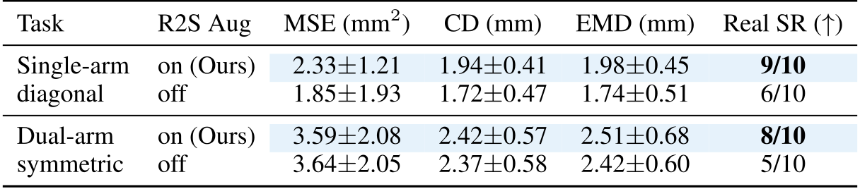
Removing augmentation slightly improves some synthetic metrics but reduces hardware success from 9/10 to 6/10 for single-arm folding and from 8/10 to 5/10 for dual-arm folding. For example, single-arm synthetic MSE improves from 2.33 to 1.85 mm² without augmentation despite worse real outcomes.
The result is consistent with appearance randomization reducing the visual sim-to-real gap, while synthetic error alone is an incomplete deployment predictor. Ten trials per setting and a combined augmentation intervention limit statistical and component-specific conclusions.