SkyJEPA learns drone dynamics from simulated state–action histories, predicts their future in a compact latent space, then converts frozen latent predictions into physical states using a structured prober. A sampling-based controller uses those states to choose actions. Outdoor flights test simulation-only training without real-flight fine-tuning. This is a low-dimensional state-based control system, not a camera-based visual world model, and its measured robustness is not a general flight-safety guarantee.
I Introduction
A useful controller needs more than a low one-step prediction loss: it needs repeated forecasts that stay useful, physically meaningful outputs and enough speed to evaluate many possible actions. SkyJEPA addresses those requirements with three connected pieces: multi-step latent learning, a physics-inspired state readout and diverse simulation data. The evidence comes from open-loop predictions and real closed-loop tracking, each of which tests a different part of the system.
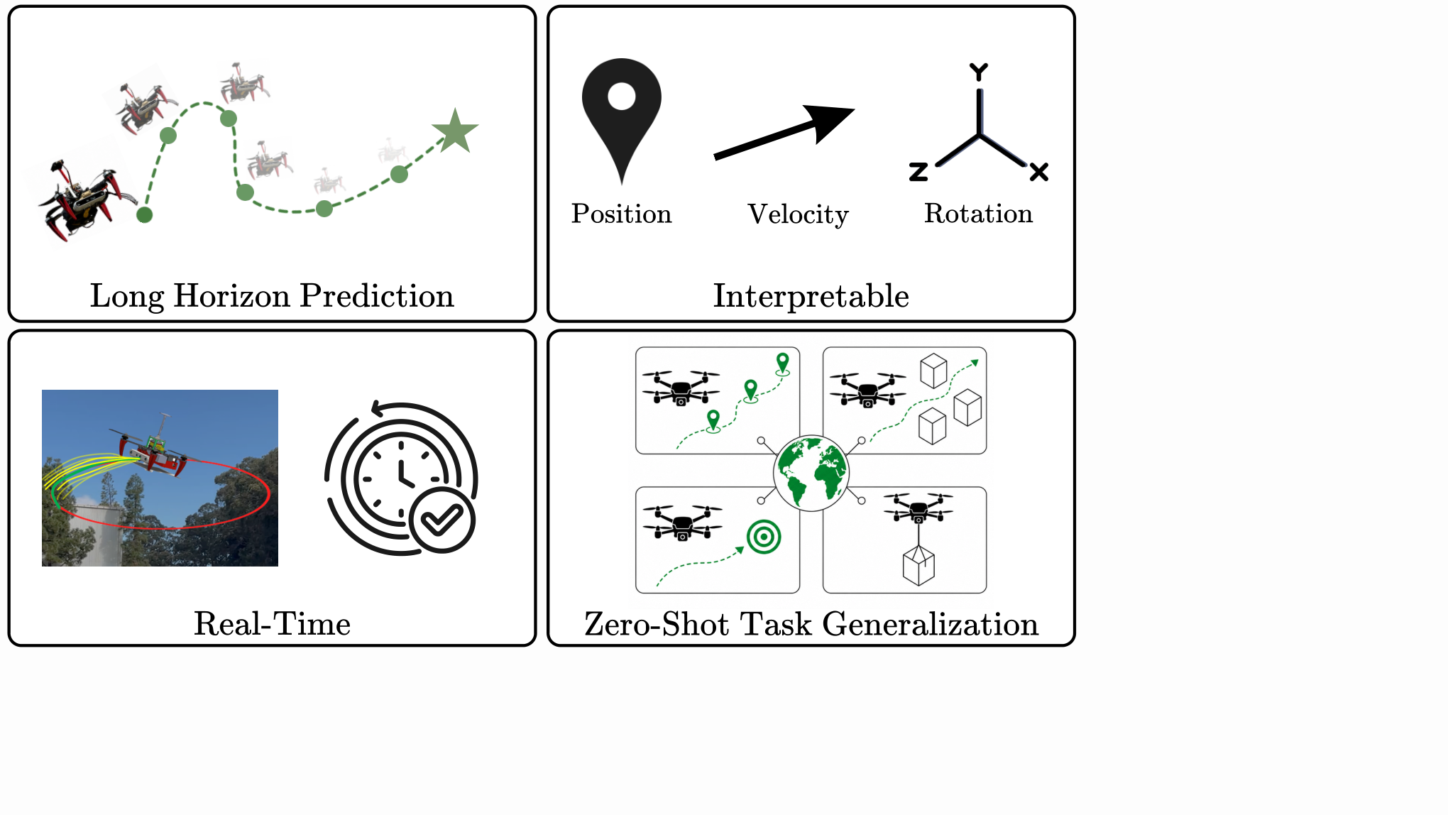
Figure 1: Desirable properties of a quadrotor world model: accurate long-horizon prediction, interpretable, real-time inference for closed-loop control, and zero-shot task generalization.
II Related Works
The comparisons distinguish the space in which dynamics are learned, the information used to train them and whether the model is specialized to a reward. These choices can be combined in several ways. The paper’s ablations are therefore more informative than treating all prior predictive or reinforcement-learning models as one uniform baseline.
II-A Predictive Modeling
Direct state predictors repeatedly consume their own imperfect outputs, so small errors can shift later inputs away from the training distribution. Residual models, physical penalties and online adaptation address parts of this problem. SkyJEPA instead rolls out learned representations, but it still uses a recurrent predictor. Its experiments show reduced error growth, rather than a theorem eliminating recursive prediction error.
II-B Joint Embedding Predictive Architectures
JEPA methods predict representations instead of reconstructing every observation. Here the emphasis is fast dynamics forecasting for a physical aircraft, using estimated states rather than image patches. The paper should be compared with other state-based controllers under matched sensing and hardware assumptions; success does not establish the proposed future camera-navigation extension.
II-C Model-Based Reinforcement Learning
A reward-conditioned model may learn only the details useful for one policy or objective. SkyJEPA trains its latent dynamics without a task reward, then supplies a tracking cost at planning time. That separates model training from the chosen path. The final controller is still task-dependent because its reference trajectory, cost weights and action limits specify what it should do.
III Background
The background defines the physical state and explains why recursive forecasts are harder than isolated one-step predictions. Keep the distinction between a latent coordinate and a measured physical quantity: tracking costs need position and attitude, so an additional state-recovery stage remains necessary even when prediction happens in a latent space.
III-A Learning System Dynamics
The state includes position, velocity, a 3×3 orientation matrix and body angular velocity. Four motor forces form the modeled action. Representing orientation with a rotation matrix avoids treating three-dimensional rotations as ordinary independent numbers. These quantities are supplied by the state-estimation/control stack; the learned model does not infer them from raw camera images.
Equations 1–2
(1)
(2)
III-B Predictive Modeling
A one-step model can look accurate when each input is a true recorded state. During an open-loop rollout, its input is instead the previous prediction, so an early error changes every later calculation. This is the motivation for training and evaluating multi-step predictions. It does not mean a different representation automatically becomes immune to accumulated error.
Equations 3–6
(3)
(4)
(5)
(6)
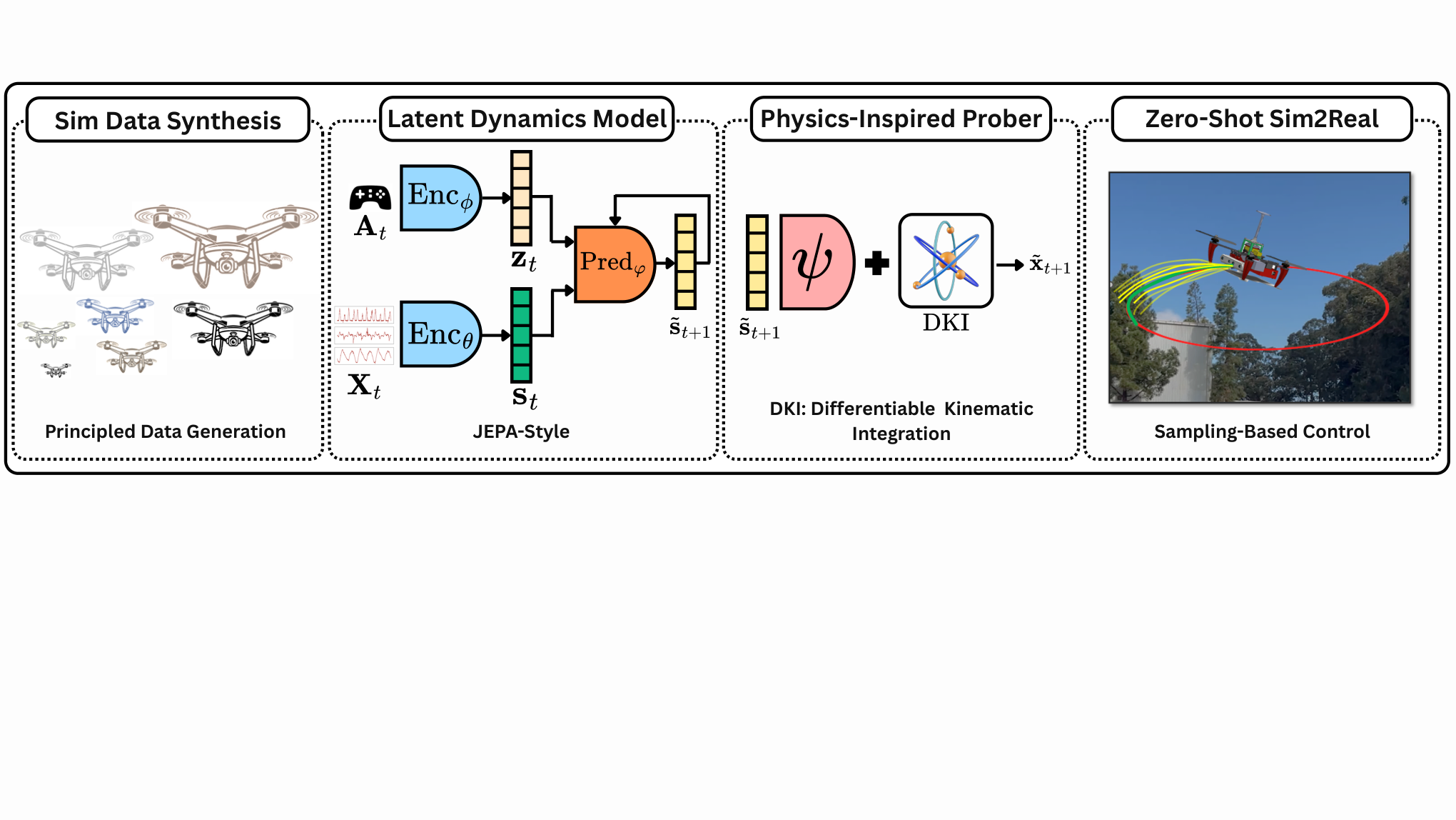
Figure 2: Overview of the proposed framework. We learn a JEPA-style latent dynamics model with a physics-inspired prober that maps abstract embeddings to physically meaningful states, enabling stable long-horizon quadrotor prediction. Trained entirely on domain-randomized simulation data and deployed within a sampling-based controller, the model achieves real-time execution and robust zero-shot sim-to-real transfer validated in outdoor flight experiments.
IV Methodology
The training and deployment pipeline has four stages: learn action-conditioned latent dynamics, fit a physical-state prober with the latent model frozen, optimize candidate controls using the combined forecast, and generate training trajectories in randomized simulators. Separating these stages makes it possible to see which information and supervision each component uses.
IV-A Problem Formulation
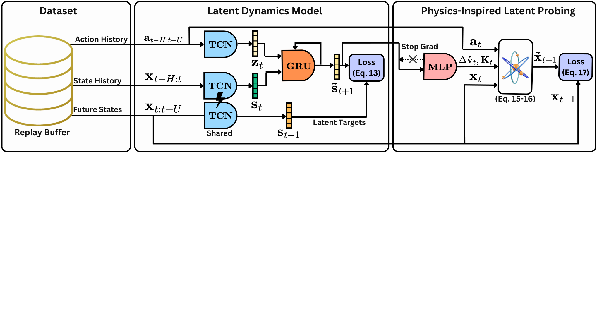
Temporal-convolution encoders summarize recent states and actions, and a recurrent predictor advances the state embedding under future actions. The history provides evidence about delayed actuators and recent motion. Prediction remains recursive in latent space, while training asks the full predicted sequence to agree with encoded future histories. The intended benefit is a representation that is easier to roll out, not the removal of recurrence.
Equations 7–8
(7)
(8)
IV-B Training Objective
The multi-step loss alone could be minimized by mapping every trajectory to a constant. SIGReg opposes that shortcut by checking whether random one-dimensional projections of the predicted embedding batch resemble a Gaussian. The ideal all-projection characterization motivates the method; finite directions, batches and quadrature approximate it. Anti-collapse regularization does not itself guarantee preservation of every unstable or safety-relevant state direction.
Equations 9–13
(9)
(10)
(11)
(12)
(13)
Figure 3: Two-stage training pipeline of our proposed approach. In the first stage, an encoder maps a history of past states into a latent representation, and a predictor propagates this latent forward in time conditioned on a sequence of control actions; in the second stage, a physics-inspired prober is trained on frozen latent embeddings to map them to physically grounded states.
IV-C Physics-Inspired Probing Mechanism
After freezing the encoders and predictor, train a small network to produce acceleration corrections from their latent rollouts. A structured integrator combines these corrections with thrust, gravity and rotation updates to recover physical trajectories. This second stage uses supervised state targets. The rotation exponential keeps attitude updates on the space of valid rotations; that geometric property does not guarantee a correct forecast under arbitrary disturbances.
Equations 14–17
(14)
(15)
(16)
(17)
IV-D Sampling-Based Control with Learned Dynamics
MPPI proposes many noisy variations of a nominal action sequence, clips them to allowed limits and rolls out each candidate through the learned dynamics and prober. Candidates with lower tracking cost receive larger softmax weights. Execute only the first updated action, obtain a new state estimate and plan again. Replanning helps correct errors, but action clamping alone does not enforce obstacle avoidance or guarantee safe states.
Equations 18–24
(18)
(19)
(20)
(21)
(22)
(23)
(24)
IV-E Automated Data Synthesis
Generate smooth random reference paths, track them with established controllers inside simulation, and record the resulting feasible state–action sequences. Randomizing mass, inertia, drag and actuator properties broadens the dynamics the learner encounters. This is more structured than independently sampling arbitrary states. Its transfer benefit still depends on whether the simulated family and sensing assumptions adequately represent the real aircraft.
Equations 25–27
(25)
(26)
(27)
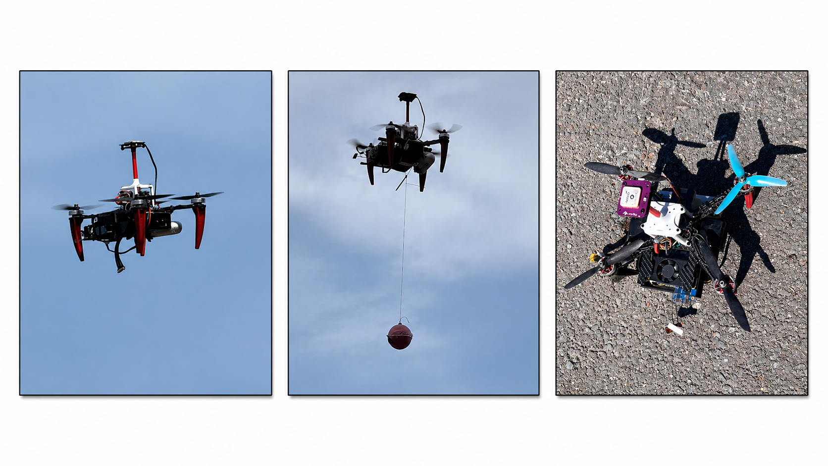
Figure 4: Closed-loop real-world evaluation settings under trajectory tracking. We test the proposed framework under three scenarios: (a) nominal trajectory tracking, (b) payload variation, and (c) propeller switching.
V Implementation Details
Implementation details matter here because three different clocks appear: the data/model sampling step, the learned rollout length and the frequency of replanning on the aircraft. They are not interchangeable. The hardware, state estimator and low-level flight controller are also part of the demonstrated system, rather than capabilities supplied by the neural model alone.
V-A Platform Setup
Experiments use a 1.3 kg quadrotor with onboard Orin NX computation, a PX4 flight controller and GPS-based state estimation. A ground laptop sends high-level commands, while the aircraft runs the control computation. Trials cover nominal tracking, a payload and changed propellers outdoors. These conditions define the demonstrated sensing and platform scope.
V-B Dataset Generation
The simulation pipeline samples 500 domains and tracks 20,000 ten-second reference trajectories. Data are resampled at 0.05 seconds, or 20 Hz, and split 80/10/10 for training, validation and testing. A held-out trajectory split evaluates new rollouts from this generated distribution; it should not automatically be interpreted as a split that holds out entire simulator parameter domains.
V-C Network Architecture and Training
Small temporal-convolution encoders feed a single-layer GRU predictor. Training uses twenty rollout steps, a one-second horizon at the 20 Hz data rate, with roughly half a second of history. The objective combines multi-step consistency and SIGReg. The compact architecture, about nine thousand parameters in the reported runtime discussion, is central to evaluating hundreds of control candidates onboard.
Table I: Domain randomization parameters used for simulation data collection.
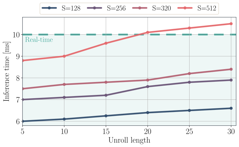
The controller is implemented in C++ and uses TensorRT for neural inference on the Jetson. The timing experiment asks which sample counts and rollout lengths fit a ten-millisecond budget. Table II lists a fifteen-step control horizon, while the runtime discussion identifies twenty steps with 512 candidates near the boundary. Keep those reported settings distinct, along with the 0.05-second prediction step and approximately 100 Hz replanning target.
VI Experiments
Open-loop tests ask whether forecasts remain accurate without measurement corrections. Closed-loop flights test whether those forecasts help a controller track paths when it repeatedly observes and replans. The study also ablates physical probing and dataset quality. Strong tracking can coexist with imperfect open-loop models, so neither metric should be used as a substitute for the other.
Figure 5: Inference speed on NVIDIA Orin NX. Inference time increases with unroll length and number of MPPI rollouts ; the selected horizon is chosen to remain below the 10 ms real-time control budget.
VI-A Latent Dynamics Modeling
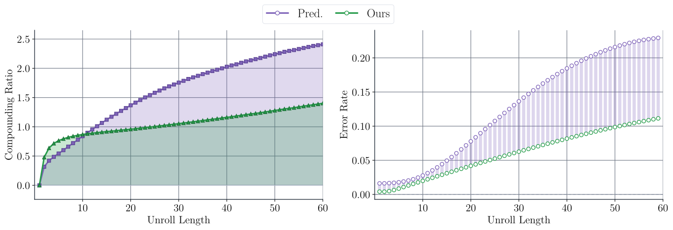
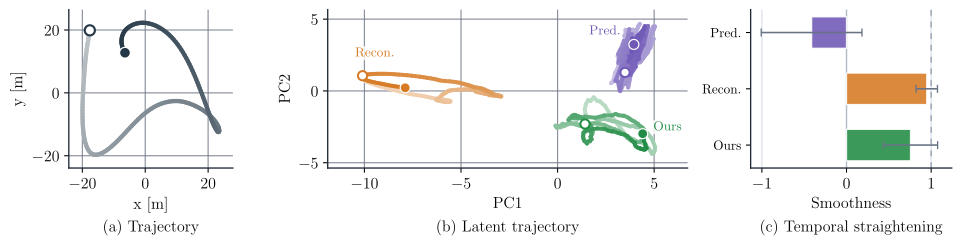
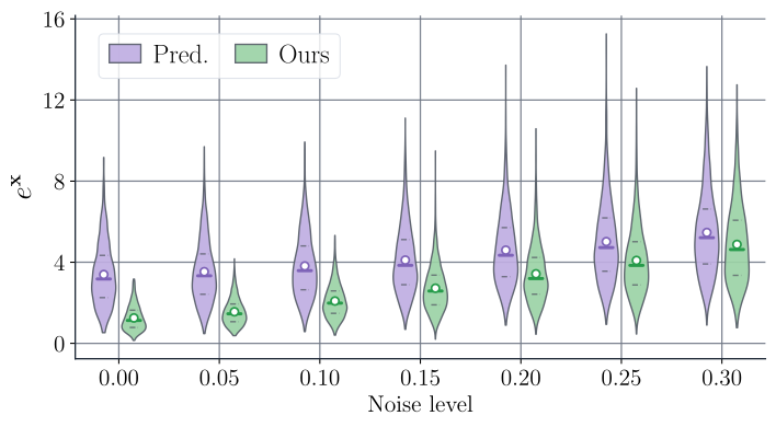
The compounding ratio compares recursive rollout error with teacher-forced error, where true past states are available; a small denominator can make early ratios unstable. At longer horizons, the latent model’s ratio and incremental error growth are lower than the direct predictor’s. Latent paths are also smoother, although the reconstruction-based latent baseline has the highest straightening score. Added Gaussian observation noise favors the full method in the tested range. These diagnostics support reduced error accumulation without establishing a universal stability bound.
Equations 28–30
(28)
(29)
(30)
Figure 6: Recursive rollout error analysis. The compounding ratio (left) compares open-loop prediction to teacher-forced prediction; values above indicate error accumulation caused by recursion. The error growth rate (right) measures the additional pose error introduced at each rollout step. Our method stays closer to teacher-forced behavior and has lower error growth than the predictive baseline, showing that latent-space dynamics modeling mitigates long-horizon compounding error.Figure 7: Temporal straightening analysis of latent rollouts. (a) Example Cartesian trajectory, with shading indicating progression from earlier to later states. (b) PCA projection of the corresponding latent trajectories, showing how each model evolves in representation space over time. (c) Temporal straightening score; higher values indicate smoother and more directionally consistent latent evolution. Temporally straighter latent trajectories suggest that complex system dynamics are represented in a simpler geometry, making recursive prediction easier and reducing directional drift during rollout.
Takeaway: Latent-space dynamics modeling reduces compounding error and has a much smaller gap between teacher-forced and recursive rollout predictions.
Equation
Takeaway: Both latent models learn temporally smoother latent trajectories than direct predictive modeling, suggesting that temporal smoothness is an important emergent property.
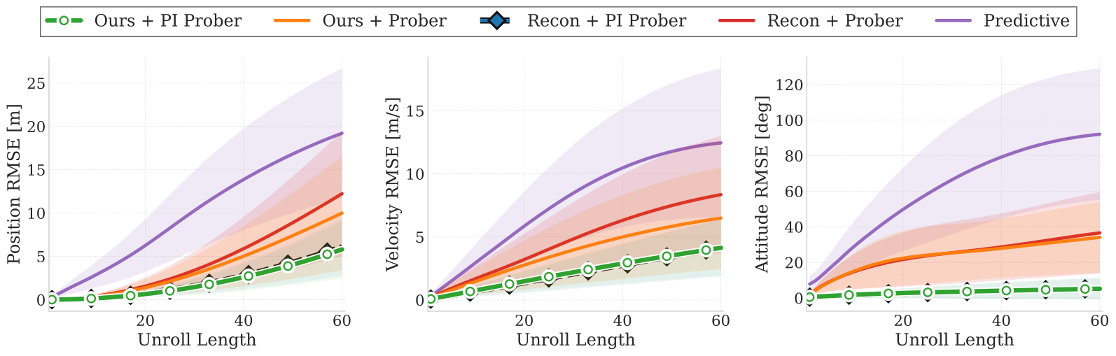
Figure 8: Open-loop rollout fidelity across dynamics models. Position, velocity, and attitude RMSE are shown versus unroll length, where lower error indicates more accurate long-horizon prediction. Direct predictive models accumulate error rapidly, especially in attitude, while latent dynamics models grow more slowly. The proposed physics-inspired prober substantially improves metric-state recovery, showing that structured physical decoding is critical for accurate state prediction.Figure 9: Robustness to observation corruption. Pose RMSE under increasing i.i.d. Gaussian observation noise, showing that the JEPA model consistently outperforms the predictive baseline and remains more robust as corruption increases.
Takeaway: Our JEPA-style approach remains more accurate under input corruption, indicating stronger robustness to corrupted inputs.
VI-B Physics Interpretability
The strongest result is the physical prober ablation: replacing a generic decoder with the structured readout cuts the JEPA model’s mean position error from 5.56 m to 1.43 m in the reported open-loop test. A reconstruction-trained latent model also improves sharply with that prober. Therefore much of the gain comes from state-recovery structure; it should not all be attributed to the JEPA objective. Attitude error measures the angle of the relative rotation, not a raw difference between matrix entries.
Table III: Open loop prediction analysis of different neural dynamics frameworks.
Table IV: Quantitative results of real-world trajectory tracking across reference trajectories. Each trajectory is executed 5 times. The mean and variance are reported.
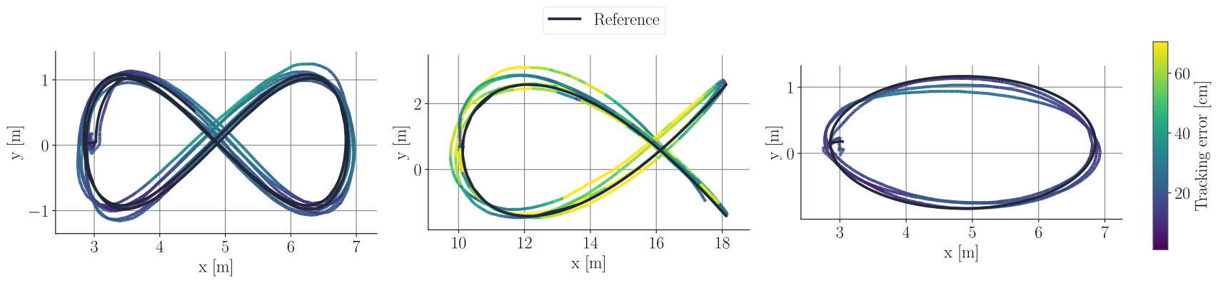
Figure 10: Real-world zero-shot trajectory tracking using the proposed controller. The plots show executed flight trajectories overlaid on the desired references. Color indicates tracking error in centimeters, with darker regions corresponding to lower error. The controller closely follows diverse real-world trajectories using a dynamics model trained only in simulation.
Takeaway: Embedding kinematic structure enables high-fidelity metric-state recovery, showing that the latent rollouts retain sufficient information to reconstruct the full dynamics.
VI-C Zero-Shot Sim-to-Real Transfer
Across five reference-path families, each repeated five times, the simulation-trained full method has lower mean position and attitude errors than the two compared predictive-model controllers. For example, circle position error is 0.24 m versus 0.39 m for the unregularized predictive baseline. Here zero-shot means no real-flight model fine-tuning. It does not mean no engineered state estimator, tracking objective, simulator design or controller tuning.
Table V: Quantitative results of closed-loop tracking under propeller switching and payload scenarios. All trajectories were executed at an average velocity of 2 ms-1 and executed 5 times. The table reports the mean and variance.
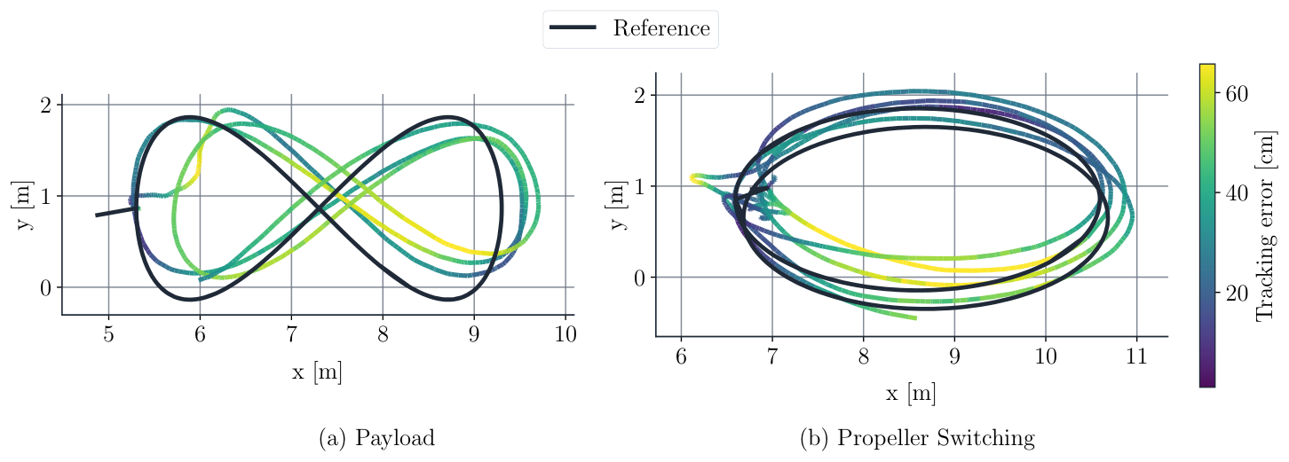
Figure 11: Real-world tracking under platform changes without retraining. (a) Payload transportation modifies the mass and inertial properties of the quadrotor. (b) Propeller switching changes the actuation characteristics. The executed trajectories remain close to the reference paths, with color indicating tracking error in centimeters. These rollouts show that the proposed framework remains effective under non-nominal deployment conditions.
VI-D Robustness
Changed propellers and a 300 g payload test two specific deployment variations without retraining. The full method tracks better than the compared controllers in the reported repeats. Those scenarios were absent as explicit data-collection configurations, but simulation already randomized mass and actuation. The results support robustness to these tests, rather than proof of transfer to every aircraft or a completely disjoint physical-parameter distribution.
Takeaway: A well covered diverse domain-randomized simulation data is sufficient for zero-shot sim2real deployment.
VI-E Data Quality
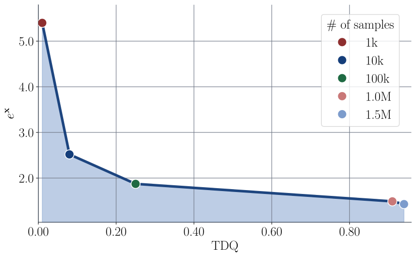
TDQ scores how broadly data occupy clusters of state–action features, local transitions and simulator parameters. Each component combines occupancy entropy with sufficient cluster coverage; a harmonic mean prevents one weak component being hidden by the others. Larger datasets have higher TDQ and lower test error here. Because size and coverage change together, the plot is a correlation, not an isolated causal test or a certified out-of-distribution coverage measure.
Equations 35–36
(35)
(36)
Figure 12: As dataset size increases, TDQ rises from to , while state RMSE decreases from to , showing that higher trajectory distribution quality correlates with better learned dynamics prediction.Equations 37–38
(37)
(38)
Takeaway: Higher TDQ leads to lower state prediction error, indicating that broader state–action coverage, richer transitions, and better parameter diversity improve learned dynamics prediction.
VII Discussion
The results support a useful combined design: simulation diversity, recurrent latent dynamics and a structured supervised state readout. The prober ablation shows that physical integration is a major contributor. Remaining questions include sensitivity to the simulated parameter family, estimator failures and disturbances beyond the tests. Neither low prediction error nor Gaussian latent regularization provides a formal control-stability or flight-safety guarantee.
VIII Conclusion and Future Works
The demonstrated contribution is state-based quadrotor dynamics and tracking with simulation-only model training. Learning from onboard RGB or depth images, navigating clutter, representing uncertainty and incorporating explicit safety constraints are proposed future directions. They should remain separate from the present outdoor path-tracking results.
64 references
[1]V. Kumar and N. Michael (2012)Opportunities and challenges with autonomous micro aerial vehicles.
The International Journal of Robotics Research31 (11).
Note: pp. 1279–1291
[2]Y. Wang, Q. Lu, and B. Ren (2023)Wind turbine crack inspection using a quadrotor with image motion blur avoided.
IEEE Robotics and Automation Letters8 (2).
Note: pp. 1069–1076
[3]K. Chua, R. Calandra, R. McAllister, and S. Levine (2018)Deep reinforcement learning in a handful of trials using probabilistic dynamics models.
Advances in Neural Information Processing Systems31.
[4]G. Williams, N. Wagener, B. Goldfain, P. Drews, J. M. Rehg, B. Boots, and E. A. Theodorou (2017)Information theoretic mpc for model-based reinforcement learning.
In IEEE International Conference on Robotics and Automation (ICRA),
pp. 1714–1721.
[5]T. M. Moerland, J. Broekens, A. Plaat, and C. M. Jonker (2023)Model-based reinforcement learning: a survey.
Foundations and Trends in Machine Learning16 (1).
Note: pp. 1–118
[6]G. Loianno, C. Brunner, G. McGrath, and V. Kumar (2017)Estimation, control, and planning for aggressive flight with a small quadrotor with a single camera and imu.
IEEE Robotics and Automation Letters2 (2), pp. 404–411.
External Links: Document
[7]J. Eschmann, D. Albani, and G. Loianno (2024)Data-driven system identification of quadrotors subject to motor delays.
In IEEE/RSJ International Conference on Intelligent Robots and Systems (IROS),
pp. 8095–8102.
[8]A. Saviolo, G. Li, and G. Loianno (2022)Physics-inspired temporal learning of quadrotor dynamics for accurate model predictive trajectory tracking.
IEEE Robotics and Automation Letters7 (4).
Note: pp. 10256–10263
[9]L. Bauersfeld, E. Kaufmann, P. Foehn, S. Sun, and D. Scaramuzza (2021)NeuroBEM: hybrid aerodynamic quadrotor model.
In Robotics: Science and Systems (RSS),
[10]P. P. Rao, A. Saviolo, T. C. Ferrari, and G. Loianno (2024)Learning long-horizon predictions for quadrotor dynamics.
In IEEE/RSJ International Conference on Intelligent Robots and Systems (IROS),
pp. 12758–12765.
[11]A. Saviolo and G. Loianno (2023)Learning quadrotor dynamics for precise, safe, and agile flight control.
Annual Reviews in Control55.
Note: pp. 45–60
[12]T. Duong and N. Atanasov (2021)Hamiltonian-based neural ode networks on the se(3) manifold for dynamics learning and control.
In Robotics: Science and Systems (RSS),
[13]A. Punjani and P. Abbeel (2015)Deep learning helicopter dynamics models.
In IEEE International Conference on Robotics and Automation (ICRA),
pp. 3223–3230.
[14]L. Hewing, J. Kabzan, and M. N. Zeilinger (2019)Cautious model predictive control using gaussian process regression.
IEEE Transactions on Control Systems Technology28 (6).
Note: pp. 2736–2743
[15]J. Fu, S. Levine, and P. Abbeel (2016)One-shot learning of manipulation skills with online dynamics adaptation and neural network priors.
In IEEE/RSJ International Conference on Intelligent Robots and Systems (IROS),
pp. 4019–4026.
[16]A. Saviolo, J. Frey, A. Rathod, M. Diehl, and G. Loianno (2023)Active learning of discrete-time dynamics for uncertainty-aware model predictive control.
IEEE Transactions on Robotics40.
Note: pp. 1273–1291
[17]L. Wang, E. A. Theodorou, and M. Egerstedt (2018)Safe learning of quadrotor dynamics using barrier certificates.
In IEEE International Conference on Robotics and Automation (ICRA),
pp. 2460–2465.
[18]T. Lew, A. Sharma, J. Harrison, A. Bylard, and M. Pavone (2022)Safe active dynamics learning and control: a sequential exploration–exploitation framework.
IEEE Transactions on Robotics38 (5).
Note: pp. 2888–2907
[19]M. O’Connell, G. Shi, X. Shi, K. Azizzadenesheli, A. Anandkumar, Y. Yue, and S. Chung (2022)Neural-fly enables rapid learning for agile flight in strong winds.
Science Robotics7 (66).
Note: pp. eabm6597
[20]T. Z. Jiahao, K. Y. Chee, and M. A. Hsieh (2023)Online dynamics learning for predictive control with an application to aerial robots.
In Conference on Robot Learning,
pp. 2251–2261.
[21]J. Robine, M. Höftmann, T. Uelwer, and S. Harmeling (2023)Transformer-based world models are happy with 100k interactions.
In International Conference on Learning Representations (ICLR),
[22]C. Finn and S. Levine (2017)Deep visual foresight for planning robot motion.
In IEEE International Conference on Robotics and Automation (ICRA),
pp. 2786–2793.
[23]B. Wu, S. Nair, L. Fei-Fei, and C. Finn (2021)Example-driven model-based reinforcement learning for solving long-horizon visuomotor tasks.
In Conference on Robot Learning (CoRL),
[24]S. L. Brunton, J. L. Proctor, and J. N. Kutz (2016)Discovering governing equations from data by sparse identification of nonlinear dynamical systems.
Proceedings of the National Academy of Sciences113 (15).
Note: pp. 3932–3937
[25]G. Kulathunga, H. Hamed, and A. Klimchik (2024)Residual dynamics learning for trajectory tracking for multi-rotor aerial vehicles.
Scientific Reports14 (1).
Note: pp. 1858
[26]S. Bansal, A. K. Akametalu, F. J. Jiang, F. Laine, and C. J. Tomlin (2016)Learning quadrotor dynamics using neural network for flight control.
In IEEE 55th Conference on Decision and Control (CDC),
pp. 4653–4660.
[27]N. Mohajerin and S. L. Waslander (2019)Multistep prediction of dynamic systems with recurrent neural networks.
IEEE Transactions on Neural Networks and Learning Systems30 (11).
Note: pp. 3370–3383
[28]S. Looper and S. L. Waslander (2022)Temporal convolutions for multi-step quadrotor motion prediction.
In 2022 19th Conference on Robots and Vision (CRV),
pp. 32–39.
[29]M. Assran, Q. Duval, I. Misra, P. Bojanowski, P. Vincent, M. Rabbat, Y. LeCun, and N. Ballas (2023)Self-supervised learning from images with a joint-embedding predictive architecture.
In Proceedings of the IEEE/CVF Conference on Computer Vision and Pattern Recognition,
pp. 15619–15629.
[30]A. Bardes, Q. Garrido, J. Ponce, X. Chen, M. Rabbat, Y. LeCun, M. Assran, and N. Ballas (2023)V-jepa: latent video prediction for visual representation learning.
arXiv preprint arXiv:2312.14119.
[31]M. Assran, A. Bardes, D. Fan, Q. Garrido, R. Howes, M. Muckley, A. Rizvi, C. Roberts, K. Sinha, A. Zholus, et al. (2025)V-jepa 2: self-supervised video models enable understanding, prediction and planning.
arXiv preprint arXiv:2506.09985.
[32]A. Bardes, J. Ponce, and Y. LeCun (2023)MC-jepa: a joint-embedding predictive architecture for self-supervised learning of motion and content features.
arXiv preprint arXiv:2307.12698.
[33]G. Zhou, H. Pan, Y. LeCun, and L. Pinto (2025)DINO-wm: world models on pre-trained visual features enable zero-shot planning.
In International Conference on Machine Learning (ICML),
[34]R. G. Goswami, A. Bar, D. Fan, T. Yang, G. Zhou, P. Krishnamurthy, M. Rabbat, F. Khorrami, and Y. LeCun (2026)World models for learning dexterous hand-object interactions from human videos.
arXiv preprint arXiv:2512.13644.
[35]A. Bar, G. Zhou, D. Tran, T. Darrell, and Y. LeCun (2025)Navigation world models.
In Proceedings of the IEEE/CVF Conference on Computer Vision and Pattern Recognition,
pp. 15791–15801.
[36]S. Yin, K. Yin, W. Chen, Y. Liu, G. Li, and L. Lin (2026)DDP-wm: disentangled dynamics prediction for efficient world models.
arXiv preprint arXiv:2602.01780.
[37]L. Maes, Q. L. Lidec, D. Scieur, Y. LeCun, and R. Balestriero (2026)LeWorldModel: stable end-to-end joint-embedding predictive architecture from pixels.
arXiv preprint arXiv:2603.19312.
[38]V. Sobal, W. Zhang, K. Cho, R. Balestriero, T. G. J. Rudner, and Y. LeCun (2025)Learning from reward-free offline data: a case for planning with latent dynamics models.
arXiv preprint arXiv:2502.14819.
[39]N. O. Lambert, D. S. Drew, J. Yaconelli, S. Levine, R. Calandra, and K. S. J. Pister (2019)Low-level control of a quadrotor with deep model-based reinforcement learning.
IEEE Robotics and Automation Letters4 (4).
Note: pp. 4224–4230
[40]C. Li, A. Krause, and M. Hutter (2025)Robotic world model: a neural network simulator for robust policy optimization in robotics.
In NeurIPS 2025 Workshop on Embodied World Models for Decision Making,
[41]D. Hafner, T. Lillicrap, I. Fischer, R. Villegas, D. Ha, H. Lee, and J. Davidson (2019)Learning latent dynamics for planning from pixels.
In International Conference on Machine Learning,
pp. 2555–2565.
[42]V. Micheli, E. Alonso, and F. Fleuret (2023)Transformers are sample-efficient world models.
In International Conference on Learning Representations (ICLR),
[44]A. Verraest, S. Bahnam, R. Ferede, G. de Croon, and C. De Wagter (2025)SkyDreamer: interpretable end-to-end vision-based drone racing with model-based reinforcement learning.
arXiv preprint arXiv:2510.14783.
[45]M. Krinner, E. Aljalbout, A. Romero, and D. Scaramuzza (2025)Accelerating model-based reinforcement learning with state-space world models.
arXiv preprint arXiv:2502.20168.
[46]A. Romero, A. Shenai, I. Geles, E. Aljalbout, and D. Scaramuzza (2026)Dream to fly: model-based reinforcement learning for vision-based drone flight.
In IEEE International Conference on Robotics and Automation (ICRA),
[47]F. Nan, H. Ma, Q. Guan, J. Hughes, M. Muehlebach, and M. Hutter (2025)Efficient model-based reinforcement learning for robot control via online learning.
arXiv preprint arXiv:2510.18518.
[50]A. Bardes, J. Ponce, and Y. LeCun (2022)VICReg: variance-invariance-covariance regularization for self-supervised learning.
In International Conference on Learning Representations (ICLR),
[51]J. Grill, F. Strub, F. Altché, C. Tallec, P. Richemond, E. Buchatskaya, C. Doersch, B. Avila Pires, Z. Guo, M. G. Azar, et al. (2020)Bootstrap your own latent: a new approach to self-supervised learning.
Advances in Neural Information Processing Systems33.
Note: pp. 21271–21284
[52]D. Mellinger and V. Kumar (2011)Minimum snap trajectory generation and control for quadrotors.
In IEEE International Conference on Robotics and Automation (ICRA),
pp. 2520–2525.
[53]Y. Song, S. Naji, E. Kaufmann, A. Loquercio, and D. Scaramuzza (2021)Flightmare: a flexible quadrotor simulator.
In Conference on Robot Learning,
pp. 1147–1157.
[55]L. Meier, D. Honegger, and M. Pollefeys (2015)PX4: a node-based multithreaded open source robotics framework for deeply embedded platforms.
In 2015 IEEE International Conference on Robotics and Automation (ICRA),
pp. 6235–6240.
[56]N. Wiedemann, V. Wüest, A. Loquercio, M. Müller, D. Floreano, and D. Scaramuzza (2023)Training efficient controllers via analytic policy gradient.
In IEEE International Conference on Robotics and Automation (ICRA),
pp. 1349–1356.
[57]C. Lea, M. D. Flynn, R. Vidal, A. Reiter, and G. D. Hager (2017)Temporal convolutional networks for action segmentation and detection.
In Proceedings of the IEEE Conference on Computer Vision and Pattern Recognition,
pp. 156–165.
[58]J. Chung, C. Gulcehre, K. Cho, and Y. Bengio (2015)Gated feedback recurrent neural networks.
In Proceedings of the 32nd International Conference on Machine Learning,
Vol. 37, pp. 2067–2075.
[60]Y. Wang, O. Bounou, G. Zhou, R. Balestriero, T. G. Rudner, Y. LeCun, and M. Ren (2026)Temporal straightening for latent planning.
arXiv preprint arXiv:2603.12231.
[64]J. MacQueen (1967)Some methods for classification and analysis of multivariate observations.
In Proceedings of the Fifth Berkeley Symposium on Mathematical Statistics and Probability,
pp. 281–297.