Reading guide
This edition covers all eight pages and the appendix: five figures, two exact tables, three algorithms, four equations, both full propositions and 39 references. The main distinction is between confidence about a sampled region’s unsafe volume and the collision risk of actions selected inside it. Read the guarantee conditions and fallback alongside the empirical results; the paper’s uniform-action assumption does not follow merely from selecting one action.
At a glance
X-Safe constructs local configuration-space polytopes from batched collision checks, then radially contracts a policy’s action support toward those regions. On Panda simulation and xArm7 hardware, it reduces observed collisions while preserving more task success than the RAIL comparison in simulation. It still needs calibrated robot/scene geometry, an accurate collision checker and quasi-static obstacles. Its formal result bounds the probability of excessive unsafe volume in sampled polytopes; interpreting that as policy execution risk needs additional selection/model assumptions, and the fallback is outside that guarantee.
I Introduction
A portable safeguard can reuse kinematics and a collision checker instead of learning a separate safety function for each embodiment. X-Safe seeks local safe action regions and uses an interior-directed fallback rather than always stopping. Embodiment-agnostic means sharing the procedure, not eliminating robot geometry, scene estimation, calibration or action-limit choices. Empirical performance and safety remain conditional on those inputs.
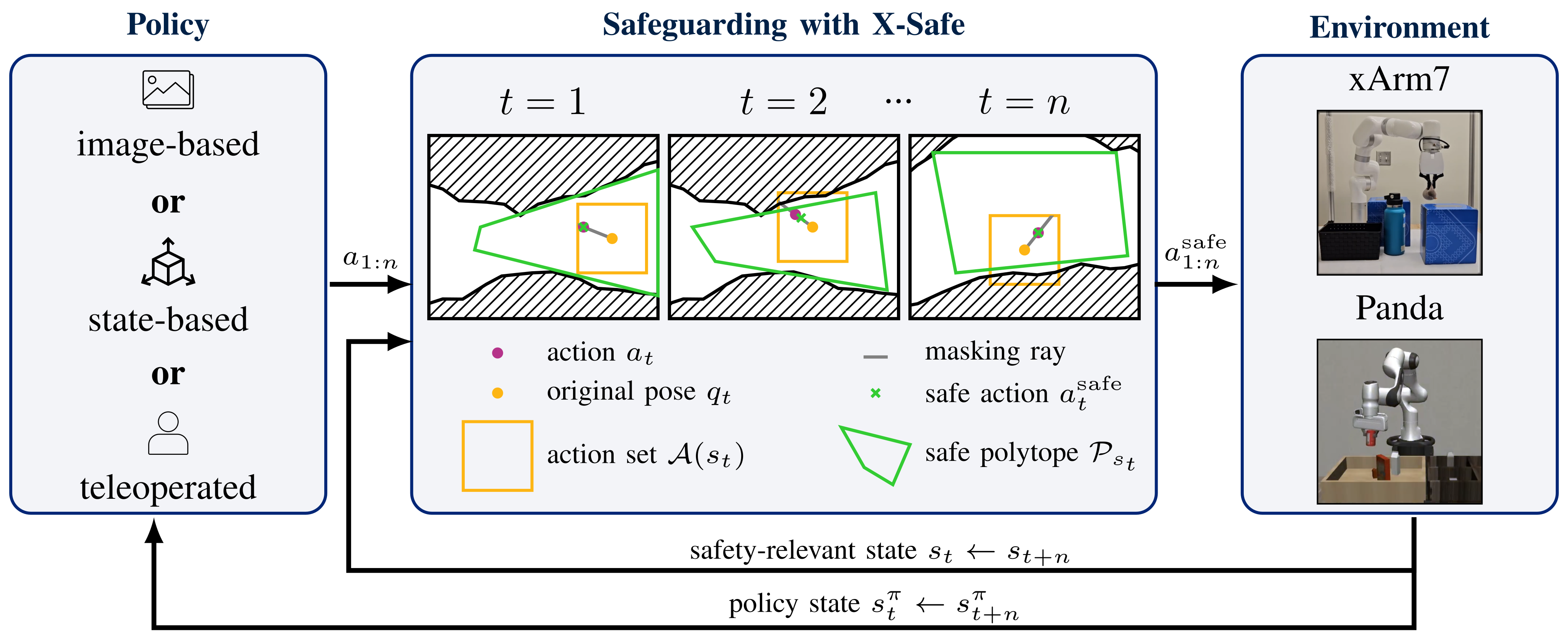
Original selectable diagram labels
- Policy
- image-based
- or
- state-based
- or
- teleoperated
- Safeguarding with X-Safe
- …
- action
- original pose
- action set
- safe action
- masking ray
- safe polytope
- Environment
- xArm7
- Panda
- policy state
- safety-relevant state
II Related Work
Projection, reachability and control-barrier methods trade different modeling assumptions, compute costs and task interference. Ray masking contracts a support set along its intended direction, avoiding the boundary mass created by ordinary projection of unsafe actions. That geometric difference does not itself prove collision freedom or make a learned policy uniform. The comparison with RAIL concerns the specific retained task and its reachability-based implementation.
III Problem Formulation
The safeguard sees joint configuration plus object poses/dimensions, which can differ from the policy’s image/state input. Actions are local joint changes bounded by per-joint limits. A MuJoCo-style twin supplies a collision predicate for proposed configurations. Equation 1 states a desired pointwise action-risk objective, while Equations 3–4 prove a different unsafe-volume confidence statement. They should not be treated as interchangeable. These definitions concern modeled configurations, not an independently proven swept-path, tracking-error, force or dynamic-obstacle guarantee.
Original mathematical definitions and guarantee conditions
We denote sets and set operations with calligraphic letters. We let the function denote the Lebesgue measure for a set and abbreviate a polytope in halfspace representation . We define the safety-relevant state comprised of a configuration , with being the degrees of freedom of the manipulator, and the object-based scene representation . The scene representation describes the pose and dimensions of objects in the environment apart from the robotic manipulator. The actions are defined relative to the current configuration of the robotic manipulator , where the action set is . Intuitively, actions are viewed, locally, as relative changes in the configuration and clipped to based on a maximum joint difference . Note that we omit the state-dependent notation for readability, and is the action set for sequential actions.
Original mathematical definitions and guarantee conditions
The violation function maps a state to if it is safe, and if a collision occurs. Thus, we can define the safe state-dependent set . Note that, in practice, the violation function is available through simulation frameworks, e.g., MuJoCo [36]. Specifically, and are used to define a virtual twin of the physical environment, and forward kinematics allow for rapidly evaluating for configurations that result from local actions . Let the policy take a state as argument and output action sequences in . Note that the state space of the policy can be different from the state space of the safeguard , e.g., a vision-based policy that uses images as state and vision-based perception that obtains for the safeguard.
Original mathematical definitions and guarantee conditions
Given the violation function , and a performant policy (i.e., near-optimal with high success rate), our goal is to construct a safe policy that satisfies a probabilistic safety guarantee. To that end, we define a safeguarding function that wraps and satisfies

Original selectable equation
Equation 1
| (1) |
Original mathematical definitions and guarantee conditions
where is a small tolerable probability of safety violation. In words, modifies such that the resulting action is safe with high probability. The probability in (1) comes from , which may be stochastic, or simply work under limited information. Of course, , i.e. stand still, satisfies (1), so another consideration for is to leverage . The safe policy, then, is given by

Original selectable equation
Equation 2
| (2) |
IV X-Safe: Probabilistic Safeguard for Manipulation
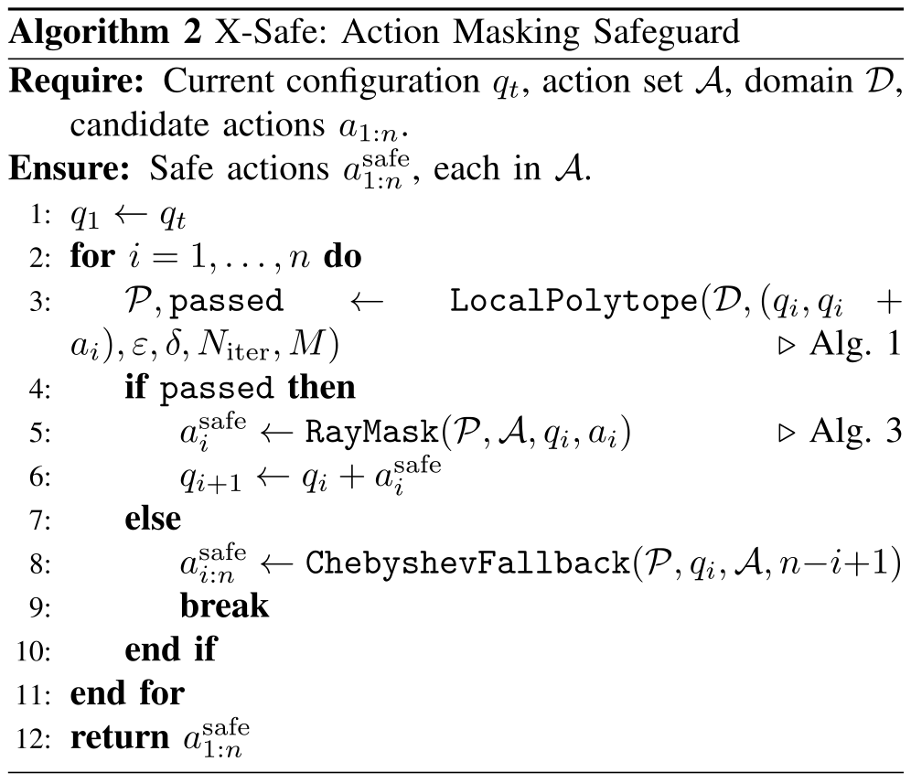
The method repeatedly samples/refines local polytopes, masks each proposed action if the test passes, and otherwise moves toward a candidate polytope’s Chebyshev center. Sequential execution uses the resulting predicted configurations. The complete statistical conditions, action masks and fallback branch remain visible in the original algorithms; the center of an unverified region is not certified collision-free by the volume theorem.
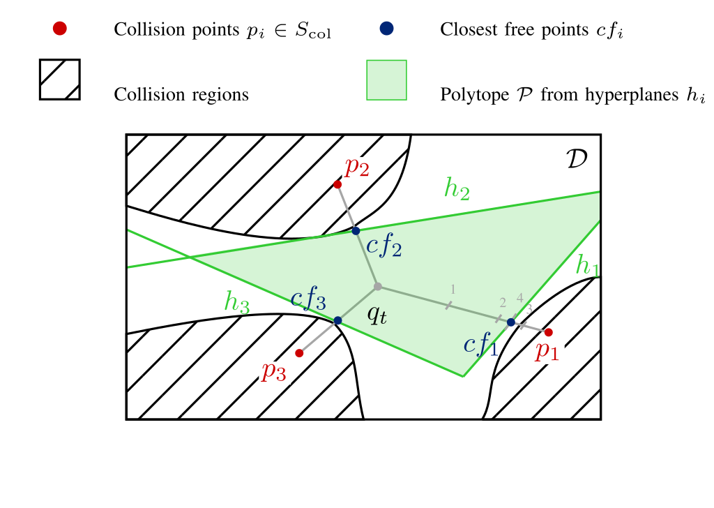
Original selectable diagram labels
- 1
- 2
- 3
- 4
-
Collision points Closest free points Collision regions Polytope from hyperplanes
IV-A Safe Polytope Computation
Uniform configuration samples drive a collision-fraction test; colliding samples produce new separating planes via bisection. The adaptation adds 4×DoF directed samples, chooses the last collision-free bisection point and returns a passed flag. Those extra samples probe relevant directions but do not make the entire region collision-free. Successful statistical termination is essential; the prose explicitly limits the guarantee when the iteration cap is reached.
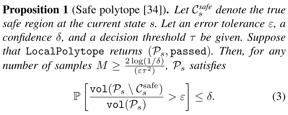
Proposition 1 bounds the probability that unsafe volume exceeds epsilon. With Table I’s delta=0.005, epsilon=0.02 and tau=0.5, its displayed sufficient sample condition requires at least 2,120 uniform samples, while the table uses M=1,024. This does not meet the printed sufficient condition. It does not prove that a separately implemented statistical test can never certify a region; that implementation/alternative justification is not supplied here.
Original mathematical definitions and guarantee conditions
We assume that safety constraints encompass self-collision and collision with quasi-static environment objects. Specifically, the unsafe set , where describes self-collisions, and describes environmental collisions, which can vary when the environment objects change, i.e., quasi-static setting. Obtaining a closed-form representation of is generally intractable in configuration space. However, the violation function , typically implemented with a simulation framework, can assess if a state , in which case it returns .
Original mathematical definitions and guarantee conditions
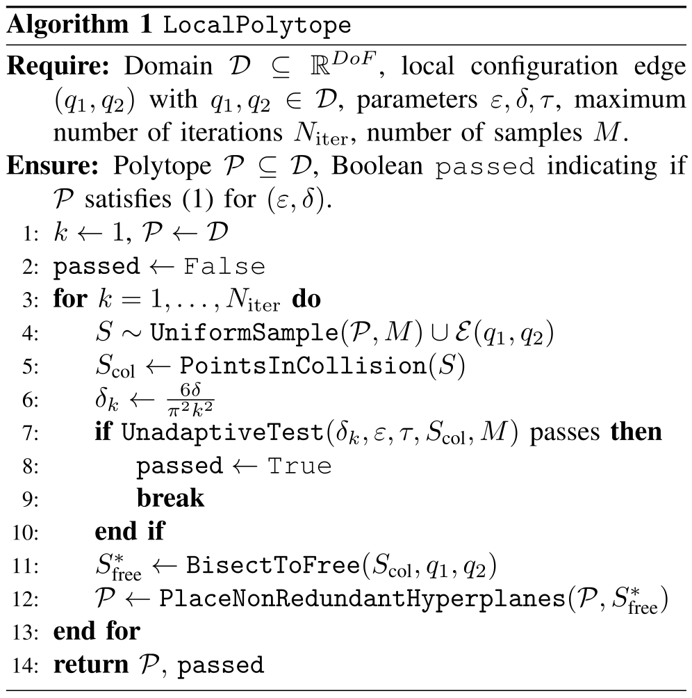
Thus, based on , we aim to define an algorithm that provides configuration space sets, locally at the current configuration, that have only a low probability of intersection with . Specifically, we adapt the sampling-based method of Edge Inflation – Zeroth Order (EI-ZO) [34, 35]. EI-ZO computes maximal probabilistically collision-free polytopes in the robot’s configuration space to build a graph of convex sets, and we adapt it to an efficient algorithm for local safe polytopes, i.e., , in Alg. 1.
Original selectable algorithm
Original mathematical definitions and guarantee conditions
In essence, EI-ZO samples points in the configuration space, counts the number of points in collision , and checks if the number of colliding points is below a threshold defined by the statistical test . The test checks if there is enough data to have confidence that the true fraction in collision is less than , given the observed samples. If the test passes, then, in all likelihood, a probabilistically safe polytope has been found. Otherwise, the collision points refine the polytope by generating additional hyperplanes at boundary points between free space and collision found by bisection (see Fig. 2). Then new samples are drawn from , and the process iterates (more details see [35]).
Original mathematical definitions and guarantee conditions
To compute the probabilistic guarantees for the polytope generated by EI-ZO, we define an admissible volume fraction which allowed to be in collision and a confidence threshold . Further, we introduce a decision threshold , which is typically set to , in order to balance the power and cost of the statistical test. Consequently, the polytope returned by EI-ZO exhibits the probabilistic guarantee stated in Prop. 1.
Original selectable proposition and assumptions
Proposition 1 (Safe polytope [34]).
Let denote the true safe region at the current state . Let an error tolerance , a confidence , and a decision threshold be given. Suppose that returns . Then, for any number of samples , satisfies
Equation 3
| (3) |
Original mathematical definitions and guarantee conditions
Intuitively, the polytope returned by the algorithm has a low probability, , of containing many unsafe states (specifically, a fraction greater than ).
Original mathematical definitions and guarantee conditions
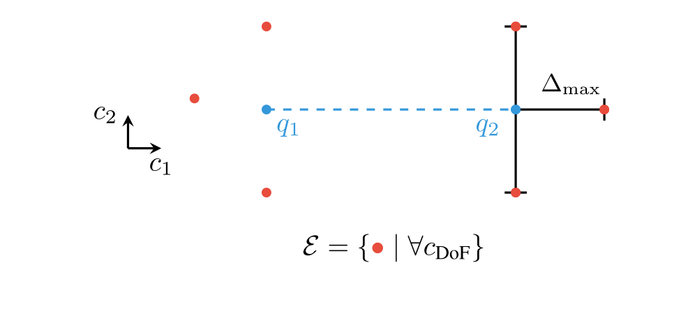
Our main adaptations to EI-ZO are threefold. First, we add the extra samples to the set of uniform configuration-space samples (Line 4, Alg. 1). In particular, the extra samples surround the local configuration edge and in axis-aligned directions (see Fig. 3). Typically, the and of interest are the current configuration and candidate action configuration . Second, we speed up termination at the expense of slightly more conservative sets by placing hyperplanes at the last collision-free point along the direction defined by and . As in EI-ZO, free points in a direction of interest are determined with bisection, but returns the last free instead of the last colliding point. Finally, the statistical test in EI-ZO (Line 7, Alg. 1) provides the probabilistic safety guarantee for the polytope stated in Prop. 1 only if the algorithm terminates within the maximum number of iterations . To detect if is sufficient to pass the statistical test, we return an additional Boolean value .
Original selectable diagram labels
IV-B Action Masking Safeguard
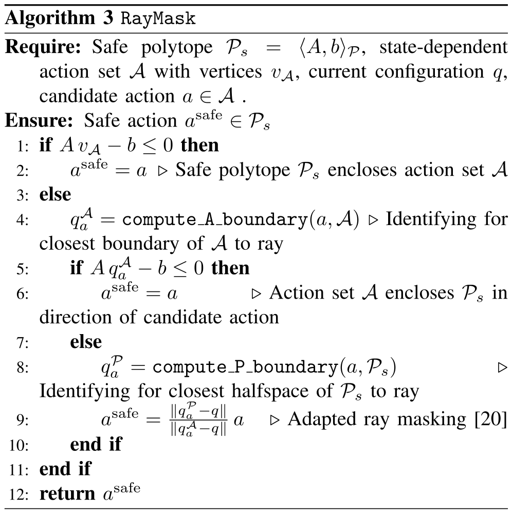
RayMask preserves the proposed direction and scales its magnitude by the ratio of polytope and action-set ray lengths when contraction is needed. It can intervene even for a currently collision-free proposal because it contracts the whole support in that direction. The resulting action distribution is generally not uniform over the polytope.
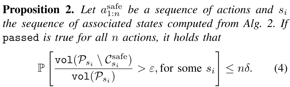
Proposition 2 applies only when all n polytope tests pass and gives an n×delta union bound on excessive unsafe volume. It does not bound arbitrary policy-action collision probability by delta. The discussion explicitly assumes uniform action selection to connect volume to risk; selecting just one point is not a proof of uniformity. A policy can concentrate on a small residual collision pocket. Even under genuine conditional uniformity, combining a good-region risk epsilon with a region-failure probability delta gives at most epsilon+delta×(1−epsilon), rather than delta alone. No density-control proof is provided for learned/adversarial RayMask outputs.
The fallback uses equal-sized steps toward the Chebyshev center when a test fails. It improves escape behavior empirically but has no retained certificate here; a failed test is not repaired mathematically by choosing an interior point.
Original mathematical definitions and guarantee conditions
Given a safe polytope, our aim is to define a safeguarding function such that only safe actions are executed. In other words, they lead to the next configuration being within the safe polytope . To this end, we draw from ray masking in [20] to correct candidate actions consistent with the intended direction in configuration space to . Effectively, ray masking radially contracts the support of the policy onto the safe polytope . The intended direction connects the current configuration and the candidate action , and is called ”ray” (see Fig. 1). Note that since the current configuration is used as the origin of the rays, ray masking will only produce a stopping action if the candidate action is the stopping action.
Original mathematical definitions and guarantee conditions
We summarize the adapted ray masking approach in Alg. 3. To efficiently determine if the ray direction requires action masking, we first check if the safe polytope fully encloses the state-dependent action set (Line 1, Alg. 3) or the polytope encloses the action set in the ray direction (Line 5, Alg. 3). In both cases, the action will remain the same, i.e., . If the action set intersects with the polytope in the ray direction, we proportionally move the actions towards the center on the ray (Line 9, Alg. 3). Intuitively, the closer the action is to the current configuration , the smaller the correction (see Fig. 1). Finally, note that projecting unsafe actions to the boundary of the safe polytope would be an alternative to masking [4, 17]. However, for stochastic policies, projection places all unsafe actions on the polytope boundary [4, Fig. 2]. Consequently, the manipulation policy would need to frequently navigate near-collision configurations, which is often challenging. In contrast, radially contracting the action distribution, as with ray masking, leads to boundary actions only if these actions were on the boundary of the action set before.
Original selectable proposition and assumptions
Proposition 2.
Let be a sequence of actions and the sequence of associated states computed from Alg. 2. If is true for all actions, it holds that
Equation 4
| (4) |
Original mathematical definitions and guarantee conditions
The proof follows directly from the union bound. In words, the probability that any of the computed polytopes contains many collisions is low. Conversely, the probability that all of them have few collisions, i.e., less than , is high, meaning at least . For longer action sequences, our confidence in the safety of all polytopes degrades. Since policies are typically executed in a receding-horizon fashion with a short action sequence, this can be counteracted by a smaller .
Original mathematical definitions and guarantee conditions
For a large number of iterations , we expect to be true. Since more iterations may prohibitively increase runtime for real-time deployment, Alg. 2 introduces a fallback controller which moves the configuration to the Chebyshev center of the candidate polytope . Specifically, the fallback controller outputs an action chunk of actions with the same magnitude, where the last action realizes the Chebyshev center. This fallback controller guides the manipulator away from unsafe configurations.
IV-C Implementation
Transfer relies on batched collision queries, a robot model and a current object-based scene twin. The domain is a local joint box, chosen as the action set in the experiments. Larger domains can see farther but require more sampling. A small confidence parameter or larger iteration budget changes the test/latency tradeoff; tuning to improve observed polytopes when tests fail is not a replacement for meeting the theorem’s conditions.
Original mathematical definitions and guarantee conditions
While our safeguard transfers easily to different embodiments and state-based as well as image-based policies, the core requirement is having access to the function , which evaluates the function for many configuration samples. In practice, this is widely accessible, e.g., when an object-based scene representation is obtained from a perception system, and the robotic manipulator is described by a Unified Robot Description Format (URDF) file [36]. Further, we need to specify the domain , which is typically an axis-aligned box centered at the current configuration. For our experiments, we found that based on maximum joint differences was most effective from both safety and performance standpoints.
Original mathematical definitions and guarantee conditions
For Alg. 1, a small leads to more iterations for convergence, and consequently increases runtime, but produces consistently better polytopes, even if did not pass. Generally, setting a large number of maximum iterations is desired so that Alg. 1 almost never reaches iterations and consequently Prop. 2 empirically holds as well. Thus, a meaningful tuning approach is to first decrease until the polytope reaches the desired refinement level, and then decrease to improve the runtime. For the parameter , we observed the least effects, and the chosen balances sampling costs and avoiding collisions well.
V Experiments
The study covers two embodiments, state/image policies and human teleoperation across four task settings. Shared defaults use M=1,024, twelve iterations, delta=0.005, epsilon=0.02 and tau=0.5; the displayed sample-bound mismatch remains. Per-step joint limits are 0.015 for Panda/adversarial xArm and 0.03 for learned xArm, selected from dimension-wise action magnitudes. These are selected operating points rather than evidence of no calibration/tuning for arbitrary robots.
Original mathematical definitions and guarantee conditions
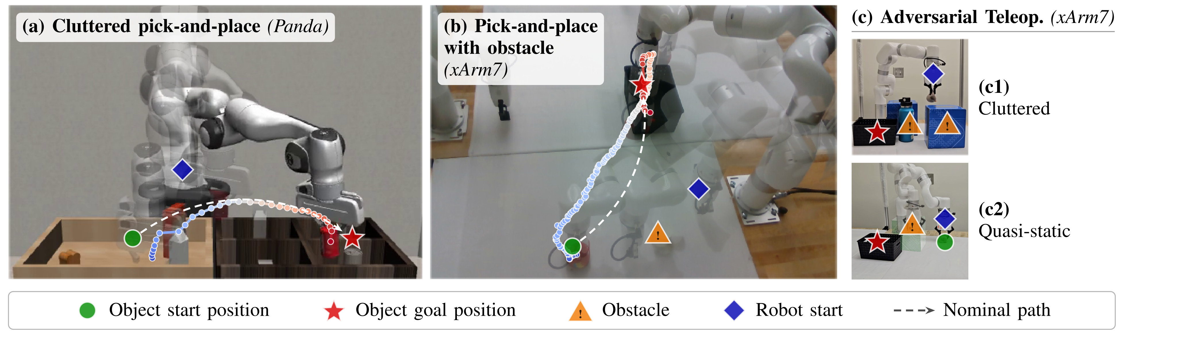
We demonstrate X-Safe on two embodiments and four tasks for state-based and image-based policies in simulation and on hardware (see Fig. 4). We specify the safeguard parameters in Table I. We set and define the width of the box based on the maximum joint differences per single step . While seemingly innocuous, this domain choice has important effects on the ray masking. If we set larger than the maximum joint differences, then we will observe collisions farther in advance. If the set defined by maximum joint differences is fully enclosed in , masking will have no effect on the action. Yet, more samples are required to adequately query the larger domain, at no additional benefit. Specifically, we set for the Franka Panda and the adversarial teleoperation on the UFactory xArm7, and for UFactory xArm7 with a learned pick-and-place policy.
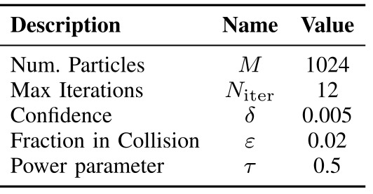
Accessible table, original values and footnotes
| Description | Name | Value |
| Num. Particles | 1024 | |
| Max Iterations | 12 | |
| Confidence | 0.005 | |
| Fraction in Collision | 0.02 | |
| Power parameter | 0.5 |
V-A Franka Panda with state-based policy
In 200 reported Panda episodes, success is 73.3% for the unsafe diffusion policy, 53.2% for RAIL and 66.4% for X-Safe: losses of 20.1 versus 6.9 percentage points. Table II reports collision fractions of timesteps, not fractions of episodes, and lists X-Safe at 0.04±0.02%; the prose instead says 0.02%. Both source values remain. Seed/aggregation details behind the reported standard errors are not fully stated.
X-Safe intervenes on 54.2% of steps versus RAIL’s 22.5%, reflecting support contraction before a proposed action necessarily collides. Its fallback runs on about 4% of steps, outside the all-tests-pass condition. Replacing that fallback with stopping drops success from roughly 66% to 44%. Episode lengths and a stated CPU/GPU setup do not substitute for a measured safeguard-latency distribution or closed-loop deadline guarantee.
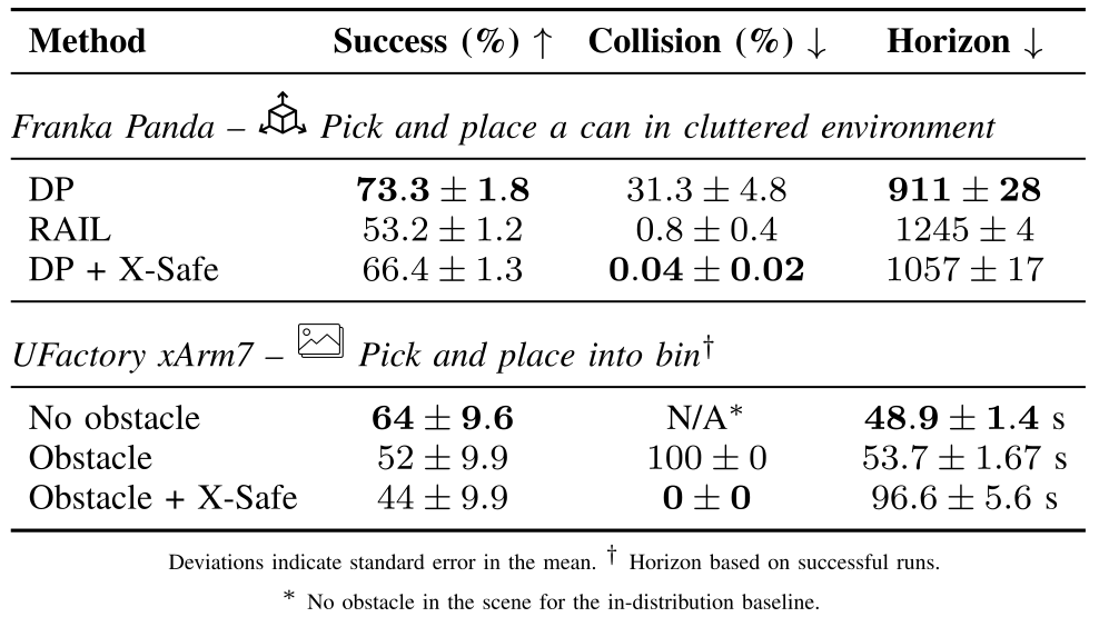
Accessible table, original values and footnotes
| Method | Success (%) | Collision (%) | Horizon |
| Franka Panda – [state observations] Pick and place a can in cluttered environment | |||
| DP | |||
| RAIL | |||
| DP + X-Safe | |||
| UFactory xArm7 – [image observations] Pick and place into bin† | |||
| No obstacle | N/A∗ | s | |
| Obstacle | s | ||
| Obstacle + X-Safe | s | ||
Deviations indicate standard error in the mean. † Horizon based on successful runs.
∗ No obstacle in the scene for the in-distribution baseline.
Original mathematical definitions and guarantee conditions
Table II presents our results. We report the task success rate per episode, the collision fraction of all time steps, and the average episode length. For the simulation experiment on the Franka Panda, we evaluated 200 episodes with maximum horizon of 2000 time steps and observed that the collision fraction with X-Safe is —lower than the expected from the formal safety guarantee. While RAIL [5] reduces the performance of the DP by compared to the unsafe benchmark, the performance drop under X-Safe is only . This is also reflected by the shorter average horizon for X-Safe. The intervention rate of X-Safe is percent of the time steps, which is higher than for RAIL. However, this is expected since action masking corrects actions when the free configuration space in the action direction is smaller than the action set, independent of the safety of the proposed action. Resulting in a look-ahead that essentially slows down the robot when approaching an unsafe region. In contrast, RAIL only intervenes when the proposed action sequence would lead to a collision, reflected by a lower intervention rate of percent. Lastly, we investigate the effect of the Chebyshev fallback controller, which is used on average for of the time steps. If we replace our fallback controller with a stopping fallback controller, the performance reduces from to as the arm deadlocks close to obstacles.
V-B UFactory xArm7 with image-based policy
A visuomotor diffusion transformer learns from 100 teleoperated demonstrations. Each hardware condition has 25 trials: success is 64% without the obstacle, 52% with it, and 44% with X-Safe. The obstacle baseline collides in every run; the safeguarded condition has zero observed collisions. Those finite counts do not establish zero deployment risk. Safeguarded failures include livelock between policy and fallback directions.
Successful safeguarded runs average 96.6 seconds versus 53.7 seconds for the obstacle baseline; these times condition on success, unlike a general per-episode latency measure. A 0.005 joint-space boundary margin triggers fallback even for passed polytopes. A separate homography-based obstacle estimate with 2 mm inflation yields zero collisions in twenty trials; this is a tested calibration setting, not a formal perception-error bound for all scenes.
Original mathematical definitions and guarantee conditions
We evaluate two different settings on a UFactory xArm7. First, we safeguard an image-based DP for a pick-and-place task. In particular, we augment the original obstacle-free task with a cylindrical obstacle that intersects with the typical path of the DP policy (see Fig. 4). To train an imitation learning policy, we collected 100 rollout demonstrations via teleoperation. The architecture of the policy is a conditional diffusion transformer model [37]. We use a standard score-matching reconstruction loss to train a visuomotor diffusion transformer that conditions on images and produces desired joint angles (in configuration space) and the gripper state. To increase the safety margin on hardware, we check if the infinity norm of the action to the polytope boundary is less than , and switch to the Chebyshev fallback controller in this case, i.e., even with polytopes that passed the statistical test.
Original mathematical definitions and guarantee conditions
For pick-and-place with xArm7, we evaluated 25 runs on hardware for each of the three settings (see Table II). The baseline without the obstacles succeeds of the runs. Once the obstacle is introduced, the policy is operating out of the training distribution, which results in a performance drop to and collisions with the obstacle or table in every run. Specifically, the obstacle is hit in every run with varying severity (i.e., small contact forces to pushing the obstacle to fall over), and the table is hit in of the runs. When using X-Safe, the task is successfully executed in of the runs, and no collisions are observed. X-Safe trades 8 percentage points of success for the elimination of all collisions. The remaining task failures originate from a livelock: the fallback controller and the DP push in nearly opposite directions near the obstacle, loops away and toward the obstacle. The increased time horizon for a run with X-Safe originates from slower operation around the obstacle. This is also reflected by the intervention rate of percent for successful runs, where interventions occur when the robot operates over the obstacle and to avoid table collisions before picking up the object. In addition, we investigated the impact of perception uncertainty by calibrating camera-to-workspace estimates using homography. With the calibration, we estimated the obstacle’s position and inflated the obstacle by , which reflects the calculated calibration error. When re-running the experiment with X-Safe and the estimated position, we observed no collisions in 20 runs.
V-C UFactory xArm7 with adversarial teleoperation
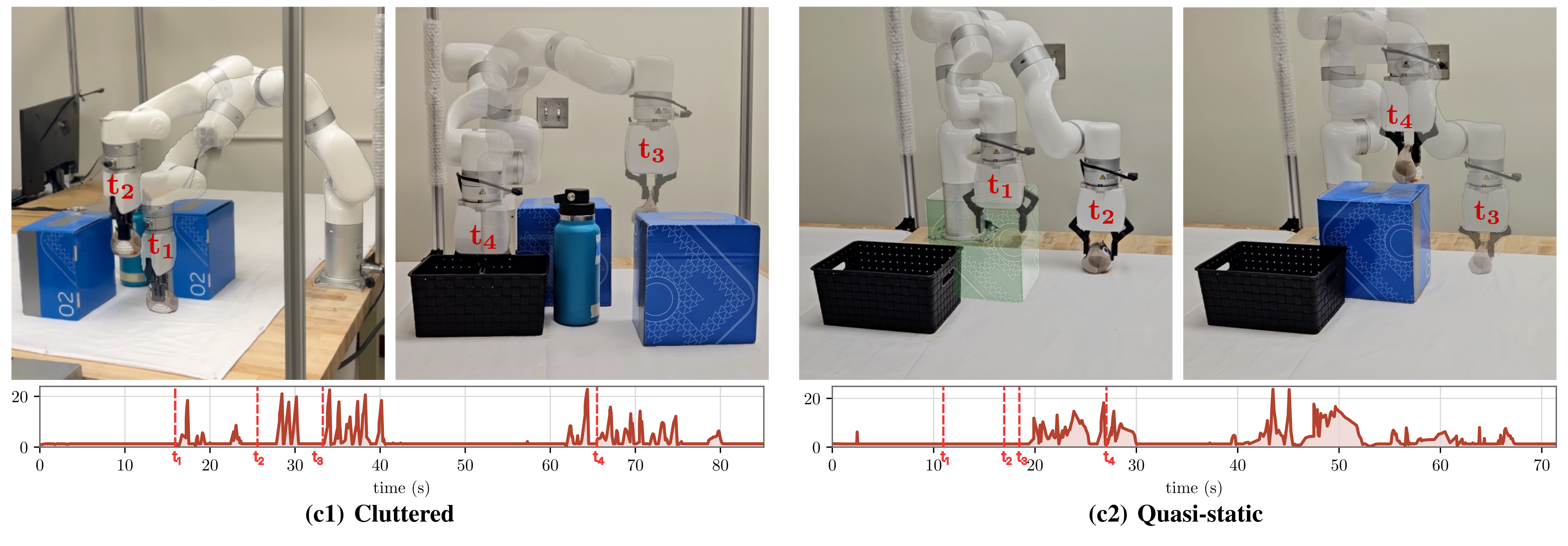
Human commands are absolute end-effector poses with downward-fixed orientation, converted by inverse kinematics to joint changes before masking. The clutter and newly introduced obstacle examples demonstrate selected guarded interactions. Quasi-static protection uses the updated virtual obstacle after perception detects it; dynamic-human motion and detection latency are not covered by the current result. No separate teleoperation trial denominator or broad adversarial stress distribution is reported.
Original mathematical definitions and guarantee conditions
We use a 3DConnexion Spacemouse to guide the robot. The Spacemouse commands are given as absolute end-effector poses. To extract joint configurations from these poses, we use the inverse kinematics solver from [38]. The target orientation is fixed to point down to simplify teleoperation. These actions, which are the difference between the target configuration and current configuration, are then ray masked to yield . The resulting target configuration, is passed to the controller as a desired joint position.
Original mathematical definitions and guarantee conditions
Fig. 5 illustrates the teleoperated manipulator experiments. The human operator adversarially moves the arm toward obstacles to demonstrate the tightness of X-Safe interventions. For the cluttered environment (i.e., Fig. 5.c1), the manipulator can grasp between three objects. When the adversarial human is trying to hit the obstacle, the Chebyshev fallback controller consistently moves the arm away from collision. Additionally, we present a quasi-static environment (i.e., Fig. 5.c2). Once detected in the physical scene, an obstacle is added to the virtual environment simulated in parallel for the collision checking function . Consequently, on the path to the bin, the adversarial operator can no longer take the shortest path because X-Safe prevents them from hitting the obstacle.
VI Discussion
The authors explicitly identify collision-predicate availability and perception-to-twin integration as central assumptions, and leave dynamic obstacles/spilling to future work. They also explicitly assume uniform action selection to interpret safe volume as action risk. Their rationale—one action selected per polytope—and low observed collision fractions do not establish that an arbitrary learned/adversarial policy is uniform or density-bounded. Extra directed samples help empirically without proving that bridge. Post-training masking changes the policy’s action distribution and reduces success; integrated training is proposed rather than evaluated.
Original mathematical definitions and guarantee conditions
The central assumption in X-Safe is the availability of the function . To implement , we use the simulation framework MuJoCo [36], which allows us to easily represent different environments and embodiments, compute forward kinematics, and check for collisions. However, the integration becomes more involved for quasi-static environments, where perception has to detect safety-relevant environmental changes and translate them into simulation objects. Further, for dynamic obstacles, like humans, or more diverse notions of safety, like not spilling liquid, future work is needed to identify rapidly evaluable violation functions .
Original mathematical definitions and guarantee conditions
The safety guarantee provided in Prop. 2 assumes uniform action selection from the safe polytope. Since only one action is selected from each polytope, the uniform assumption is reasonable, and our experimental evaluation confirmed this by producing lower collision rates than expected under the proposition. Additionally, the added samples ensure a coverage surrounding the intended robot path, which supports detecting collisions in this relevant region. Nevertheless, further empirical validation would be beneficial to substantiate that the assumption is conservative on a broader set of tasks, policies, and embodiments.
Original mathematical definitions and guarantee conditions
We used the parameters reported in Table I across tasks and embodiments to show that those can be set without significant tuning. The set is varying according to , where we took the percentile magnitude of actions, dimension-wise. The trade-off for is that smaller reduces the number of samples required, while increasing the chance of adjusting more of the support of the policy. We defer the optimization and other parameters to future work, as our goal is to demonstrate the ease of implementation and ability to transfer to other manipulators.
Original mathematical definitions and guarantee conditions
Our experiments investigate the effect of X-Safe post-training for a limited number of tasks. We consistently observe a performance reduction of varying significance. This is expected as a posteriori safeguarding changes the distribution compared to the policy’s training. To mitigate these distribution-shift effects, future work should fine-tune or train with X-Safe. Note that the differentiability of the function allows for considering X-Safe as part of the environment, [39, 17] or as part of the policy [20].
VII Conclusion
X-Safe shows useful collision reduction and a less damaging simulation safeguard tradeoff on the tested platforms. Its portable local-geometry procedure still depends on accurate scene/robot models, successful tests, compatible sample settings and an action-selection interpretation. The paper’s conclusion should be read with those formal conditions and its uncertified fallback, finite hardware trials and remaining livelocks. The complete original statements remain alongside these short notes.
Appendix: Ray masking algorithm
Algorithm 3 retains every enclosure test, ray-boundary computation and the full distance-ratio scaling rule. A printed comment on the second enclosure branch reverses the stated containment direction; the actual inequality checks whether the action-set boundary point is inside the polytope. The geometric map contracts support and preserves proposed direction where its ray lengths are defined; it is not a uniform random sampler or an independent collision checker.