At a glance
S-JEPA predicts soft acoustic-cluster distributions at masked positions. It begins with a fixed MFCC mixture, then updates a mixture online from averaged encoder features while choosing the representation layer adaptively. A 51.8 million-parameter encoder performs strongly among the compared smaller speech models. The method differs from the January precursor: its target is categorical KL prediction rather than a combined latent-regression and fixed-anchor loss.
1 Introduction
Hard cluster labels discard uncertainty when a sound frame lies between acoustic categories. S-JEPA keeps probabilities over possible categories and trains a predictor to reproduce them. The engineering aim is useful compact speech features without a repeated stop-and-recluster pipeline. Soft targets are acoustic information, not human-supplied phoneme or word labels.
2 Related Work
The lineage combines masked speech prediction, soft clustering and teacher averaging. The paper explicitly connects to the earlier GMM-anchored precursor but changes its objective and training procedure. Its relationship to JEPA is the encoder–predictor masked-prediction pattern; the target itself is a categorical distribution.
3 Method
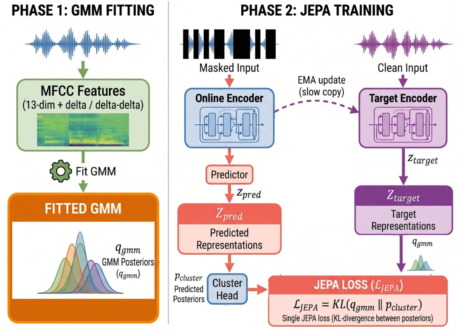
The method needs three pieces: the encoder–predictor architecture, a probability-matching objective and a continuous two-phase target-update recipe.
3.1 Architecture
The encoder processes waveform frames, a predictor fills masked positions, and a small head outputs cluster probabilities. An EMA encoder is maintained for the second phase’s target features. Training-only predictor and cluster components are discarded for ordinary encoder inference.
Equations 1–2
| (1) | ||||
| (2) |
3.2 Soft Targets and KL Loss
The target is a soft posterior over GMM components. KL divergence matches the predicted distribution to that target, preserving ambiguity a hard argmax label would remove. Which positions contribute to the loss changes during training, so the final masked-only configuration should not be described as the entire training history.
Equations 3–4
| (3) |
| (4) |
3.3 Two-Phase Training
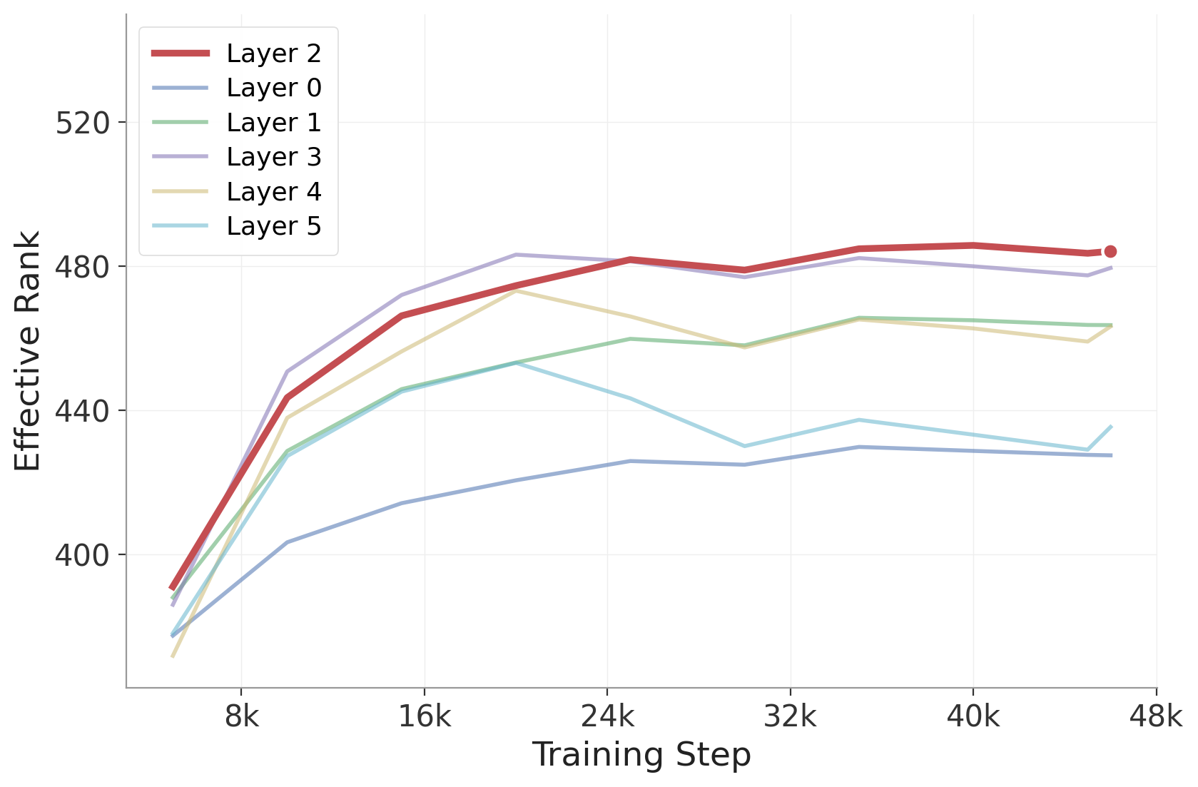
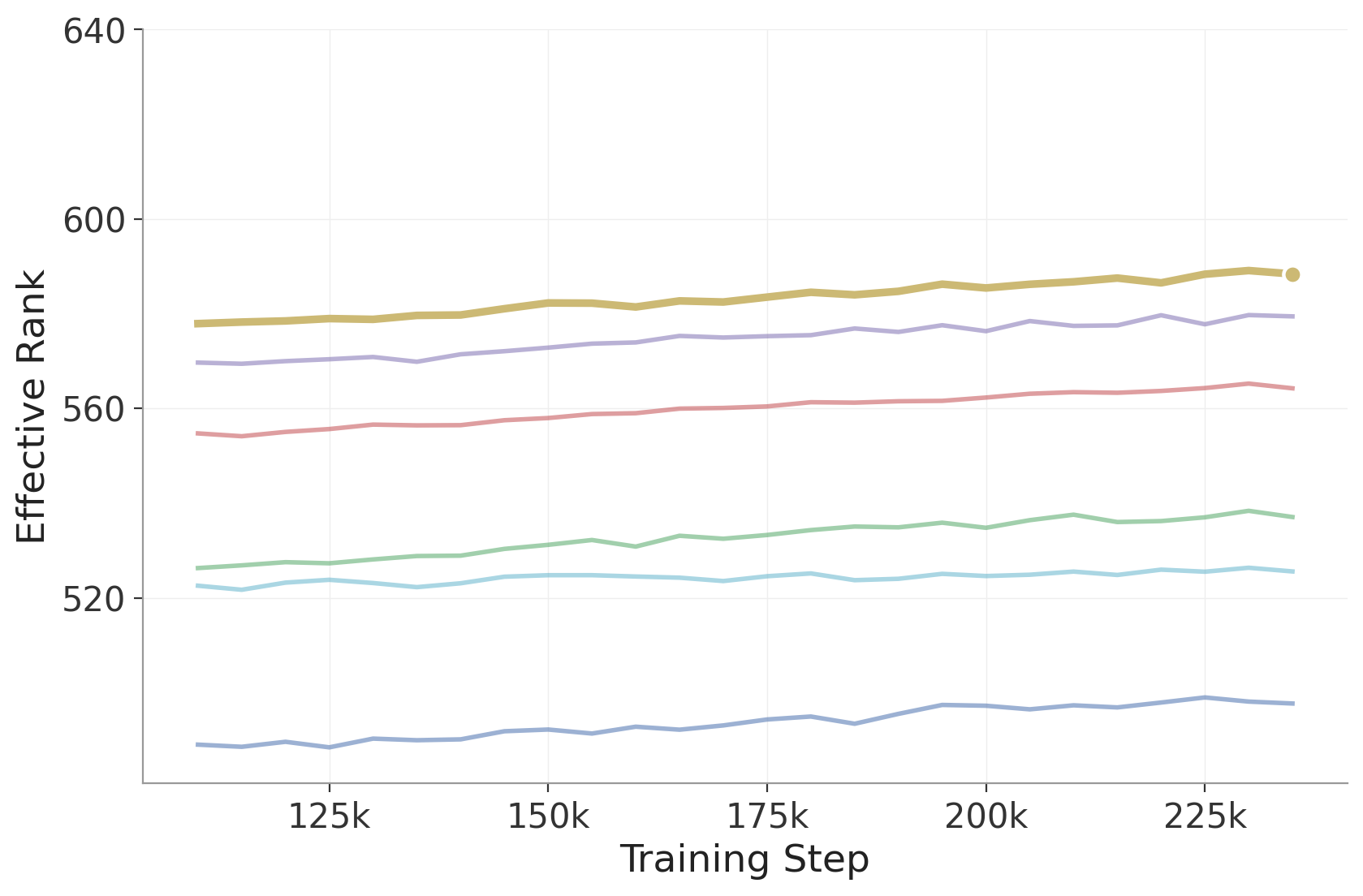
Phase 1 fits a fixed mixture to MFCC features. Phase 2 initializes a mixture over EMA encoder features, updates it online and chooses its input layer using effective-rank measurements. A periodically switched teacher-averaging rate changes how rapidly the targets follow the student. These components form a recipe, not independently established causes of the measured gain.
Equation 5
| (5) |
3.4 Training Algorithm
The algorithm makes the phase transition, masked-position updates and target-averaging schedule explicit. No gradients flow through the GMM updates; mixture statistics follow their own update rule.
4 Experiments
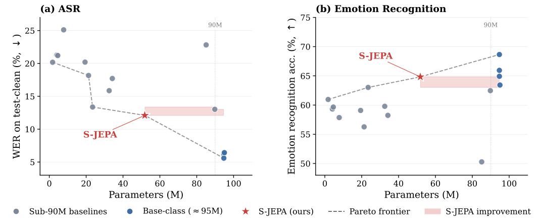
Pretraining uses approximately 83,000 hours of English speech. Evaluation freezes the 51.8 million-parameter encoder and trains smaller task-specific heads under SUPERB protocols. Parameter comparisons count inference encoders, not every teacher, predictor or pretraining computation used by alternative methods.
| Method | # Params | ASR | ER | SF | SF |
|---|---|---|---|---|---|
| WER () | Acc. () | F1 () | CER () | ||
| Sub-90M baselines | |||||
| modified CPC [39] | 001.8M | 20.18 | 60.96 | 71.19 | 49.91 |
| APC [11] | 004.1M | 21.28 | 59.33 | 70.46 | 50.89 |
| VQ-APC [12] | 004.6M | 21.20 | 59.66 | 68.53 | 52.91 |
| PASE+ [33] | 007.8M | 25.11 | 57.86 | 62.14 | 60.17 |
| NPC [27] | 019.4M | 20.20 | 59.08 | 72.79 | 48.44 |
| TERA [29] | 021.3M | 18.17 | 56.27 | 67.50 | 54.17 |
| DistilHuBERT [8] | 023.5M | 13.37 | 63.02 | 82.57 | 35.59 |
| wav2vec [35] | 032.5M | 15.86 | 59.79 | 76.37 | 43.71 |
| vq-wav2vec [2] | 034.2M | 17.71 | 58.24 | 77.68 | 41.54 |
| Mockingjay [28] | 085.1M | 22.82 | 50.28 | 61.59 | 58.89 |
| DeCoAR 2.0 [26] | 089.8M | 13.02 | 62.47 | 83.28 | 34.73 |
| S-JEPA (ours) | 051.8M | 012.10 | 64.83 | 83.05 | 33.17 |
| Base-class (95M) | |||||
| HuBERT Base [20] | 094.7M | 06.42 | 64.92 | 88.53 | 25.20 |
| WavLM Base [9] | 094.7M | 06.21 | 65.94 | 89.38 | 22.86 |
| WavLM Base+ [9] | 094.7M | 05.59 | 68.65 | 90.58 | 21.20 |
| wav2vec 2.0 Base [3] | 095.0M | 06.43 | 63.43 | 88.30 | 24.77 |
| Large-class (reference, 316M) | |||||
| HuBERT Large [20] | 316.6M | 03.62 | 67.62 | 89.81 | 21.76 |
| WavLM Large [9] | 316.6M | 03.44 | 70.62 | 92.21 | 18.36 |
| wav2vec 2.0 Large [3] | 316.6M | 03.75 | 65.64 | 87.11 | 27.31 |
4.1 Frozen-Encoder Results on SUPERB
Greedy CTC recognition reaches 12.10% WER in the reported setup; the lower 8.50% result uses language-model rescoring and is a separate setting. The model has the best WER among the compared sub 90 million-parameter systems and strong emotion recognition. Slot-filling F1 is close to, but slightly below, DeCoAR2.0; the narrative’s broad dominance wording should not hide that table entry.
4.2 Probing Frozen Representations
Frozen-feature probes test speaker, gender, chapter and phoneme information. A linear probe favors a different phoneme model than a nonlinear probe, showing that readout capacity changes what information appears accessible. Random splits within the evaluation corpus and task-specific supervised labels define the scope of the comparison.
5 Analysis
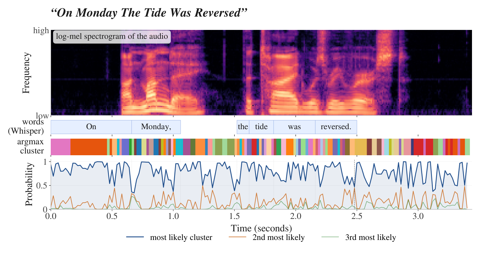
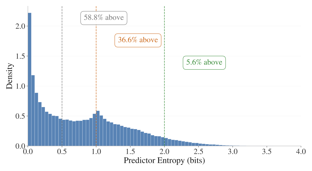
The analysis studies one illustrative utterance and an aggregate distribution of frame-level uncertainty. These answer different questions: what a particular prediction looks like and how often uncertain predictions occur.
5.1 Per-utterance Interpretability
The plotted word timings come from an external Whisper system used only for visual reference. They do not supervise S-JEPA or supply its quantitative scores. Rapid changes in cluster ID also show why the unsupervised categories should not be treated as one-to-one phoneme labels.
5.2 Aggregate Distribution of Predictor Uncertainty
Entropy across held-out frames has a confident regime and a secondary regime near a two-way tie. The reported 36.6% of frames above one bit supports preserving inter-cluster uncertainty. This is evidence about the predicted distributions; the paper leaves a matched hard-target ablation as future work.
6 Discussion
The compact model and structured uncertainty are the strongest findings. Several recipe components remain insufficiently isolated: teacher switching has no controlled alternative comparison, and augmentation and visible-position loss were changed together. English-only training limits claims about other languages and non-speech audio.
7 Conclusion
S-JEPA is a soft-target masked speech learner with online target adaptation. It supports a favorable parameter–performance tradeoff in the reported comparisons. Its mixture targets are categorical probabilities, and the remaining ablations matter when attributing gains to softness, online updates or the rest of the recipe.
Appendix A Architecture Details
The architecture largely follows HuBERT-style processing with a shallower six-layer encoder. Predictor and cluster head are training-only additions.
A.1 CNN Feature Extractor
A seven-layer convolutional frontend maps 16 kHz audio to 20 ms frames. Its stride and gradient scaling set the temporal resolution and learning balance before attention.
A.2 Transformer Stack
Six transformer layers use the stated width, heads, feed-forward size and regularization. The architecture saves encoder parameters relative to deeper base models; it does not remove transformer computation.
A.3 Encoder Mask Handling
Masked features are zeroed after the frontend/projection and before positional encoding and transformer processing. The predictor later inserts learned mask tokens. This placement is part of the implementation, not interchangeable with masking only at the final loss.
A.4 Predictor and Cluster Head
A small transformer predictor supplies hidden-position features to the cluster head. Only the specified positions receive supervision, even when the shared head is also evaluated on visible positions for analysis.
Equation
A.5 EMA Encoder
The averaged encoder is unused for Phase 1 targets and supplies target features in Phase 2. Its decay schedule affects how stationary those targets are while the online mixture adapts.
A.6 Masking
Temporal blocks hide contiguous frame spans. The target fraction and predictor-mask handling specify the prediction task’s difficulty.
Appendix B Training algorithm
The full algorithm preserves the sequence of GMM initialization, gradient updates, target averaging and layer selection. It is necessary for reproducing the continuous two-phase recipe.
Appendix C Phase 2 Transition: Masked-Only Loss and Augmentation Off
Partway through Phase 2, visible-position loss was removed and augmentation was disabled together, guided by development-set WER. Because the changes were simultaneous, their individual effects are not identified. The manuscript explicitly acknowledges this limitation.
Appendix D Training Hyperparameters
The hyperparameter table records the launch settings used for reported checkpoints. These settings include phase-specific masking, losses and schedules rather than one uniform training configuration.
| Phase 1 (MFCC GMM) | Phase 2 (online GMM) | |
| Encoder backbone (shared across phases) | ||
| Hidden dimension | 768 | 768 |
| Transformer layers | 6 | 6 |
| Attention heads | 12 | 12 |
| FFN dimension | 3072 | 3072 |
| CNN feature-extractor channels | 512 | 512 |
| CNN total stride / frame rate | 320 / 50 Hz | 320 / 50 Hz |
| Conv positional encoding (kernel, groups) | (128, 16) | (128, 16) |
| Dropout / attention / activation | 0.1 / 0.1 / 0.1 | 0.1 / 0.1 / 0.1 |
| LayerDrop | 0.05 | 0.05 |
| Feature-extractor gradient multiplier | 0.1 | 0.1 |
| GMM | ||
| (number of components) | 100 | 500 |
| Feature space | 39-dim MFCC++ | 768-dim EMA encoder features |
| Fitting | k-means init (5 it.) + EM (20 it.) | online EMA of suff. stats |
| Online param EMA decay | — (frozen) | 0.999 |
| Layer-check cadence (auto-layer) | — (n/a) | every steps |
| Optimization | ||
| Optimizer | AdamW | AdamW |
| Weight decay | ||
| Learning rate | ||
| Batch size (global) | 192 | 192 |
| GPUs | 8 | 8 |
| Max input duration | 15 s | 15 s |
| EMA encoder (periodically switched decay, Phase 2 only) | ||
| — (n/a) | 0.9999 | |
| — (n/a) | 0.999 | |
| Switching cadence | — (n/a) | every steps (avg.) |
| Masking | ||
| Mask ratio | 0.65 | 0.65 |
| Mask span length (frames) | 10 | 10 |
| Loss configuration | ||
| KL applied at | masked + visible | masked + visible (early), masked only (after) |
| Augmentation | ||
| 0.25 | 0.25 (early), 0.0 (after) | |
| 0.25 | 0.25 (early), 0.0 (after) | |
| SNR range (noise mix), dB | when active | |
| Energy ratio range (utterance mix), dB | when active | |
Appendix E GMM Details
The mixture implementation supplies probabilistic targets and updates without backpropagating through the mixture parameters.
E.1 Posterior Computation
Normalized Gaussian likelihoods produce soft assignments, with variance floors for stability. A posterior can spread mass across several plausible components.
Equation 6
| (6) |
E.2 Phase 1 GMM Fitting
Phase 1 gathers MFCC frames using bounded-memory reservoir sampling, initializes with mini-batch clustering and refines by expectation-maximization. The resulting mixture stays fixed during that phase.
E.3 Online GMM Updates (Phase 2)
Phase 2 updates component statistics from EMA-encoder features with responsibility-weighted moving averages. This replaces repeated full-corpus offline reclustering but introduces target-update dynamics of its own.
Equation 7
| (7) |
E.4 Chunked Soft Assignment
The soft-assignment calculation is split into chunks to bound peak memory. The complete source algorithm preserves the normalization and accumulation steps.
Appendix F Periodically Switched EMA Decay
Teacher decay alternates between faster and slower tracking intervals. The appendix explains the corresponding timescales and interaction with mixture updates. The schedule is a heuristic whose independent benefit was not isolated by a controlled comparison.
Appendix G Effective Rank and Adaptive Layer Selection
Effective rank is computed from normalized singular values of centered layer features, then smoothed before selecting the mixture-input layer. It measures feature-spectrum spread, not direct semantic accuracy.
Appendix H Probing Protocol
Linear and nonlinear probes are trained on frozen features using the stated splits, scaling and labels. Different readout families can reveal different recoverability of phoneme information. These probes use supervised downstream labels even though encoder pretraining is self-supervised.
Appendix I Augmentation Details
The online encoder can receive denoising augmentation while target features come from clean audio. The final second-phase recipe turns augmentation off.
I.1 Energy-Based SNR Mixing
Energy-based scaling sets a target signal-to-noise ratio before mixing clean audio with noise. The same noise amplitude would otherwise affect quiet and loud utterances differently.
Equations 8–10
| (8) | ||||
| (9) | ||||
| (10) |
I.2 Utterance Mixing
Another utterance segment is mixed at a sampled energy ratio and overlap position. This creates an acoustic denoising task rather than a new transcript target.
Equation 11
| (11) |
Appendix J SUPERB Evaluation Protocol
SUPERB trains small task-specific heads on a frozen encoder. Greedy decoding is the principal ASR comparison; optional language-model rescoring is reported separately. Matching this protocol is necessary for interpreting the baseline table.