Reading guide
All sixteen pages, six complete figures, seven tables, five equations and thirty-four references are covered. Sequential Asymmetric Imitation(SAI) first trains Robot A with compliant support, trains Robot B against that frozen policy, then refinesA with sparse corrections during joint execution. Four real-robot tasks show stronger reported success and coordination than the compared pipelines. Whole-rollout success, checkpoint synchronization and yielding opportunities have different denominators; they should not be read as interchangeable success rates or independent trials.
At a glance
Two bimanual mobile manipulators interact through rigid or deformable shared objects. A single teleoperator controls one robot at a time across a three-stage curriculum. Local policies use scene images, proprioception and torque cues without exchanging messages or predicted actions. SAI improves four-task success and event-level coordination over independent imitation and a two-stage ablation. The evidence concerns this hardware/task suite; the curriculum still needs human support, partner-aware demonstrations and failure corrections.
1 Introduction
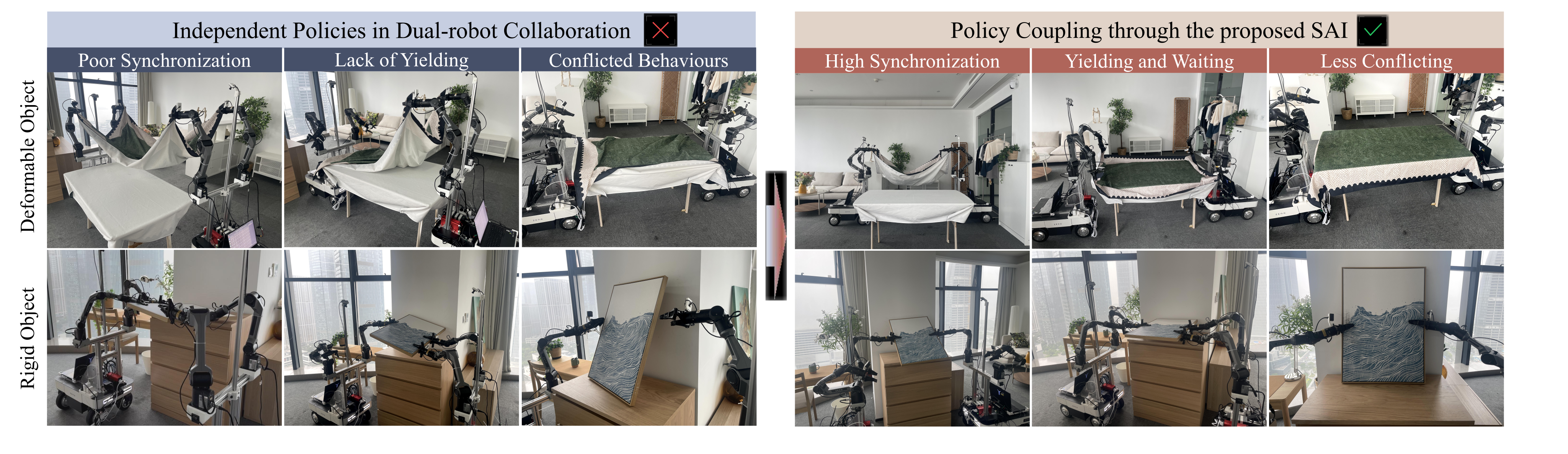
Physically coupled robots can each execute a useful skill yet fail together through mistimed pulling, lifting, release or repositioning. SAI addresses the distribution of partner behavior present in training. It avoids simultaneously teleoperating two robots but does not remove interaction-specific data collection. Shared-object dynamics and visible partner progress provide implicit coordination cues. Explicit communication is absent, while a shared top-view camera remains part of the observation system.
2 Related Work
Prior work includes model-based cooperative manipulation, visuomotor imitation, teleoperation and interactive correction. ACT, Diffusion Policy and Mobile ALOHA supply policy/interface context. DAgger motivates gathering labels under learner-induced states. SAI applies a staged partner distribution followed byA-centric corrections; the study compares complete curricula rather than proving a coordination theorem or isolating every data-volume effect.
3 Problem Formulation
Each robot chooses actions from its own visuo-proprioceptive observation/history. Policies exchange no messages, partner states, future actions or latent embeddings. Coupling arises through the observed shared workspace and physical object interaction. The three practical requirements are phase alignment, partner-contingent yielding and conflict mitigation. Single-teleoperator supervision creates three datasets, not a synchronized joint demonstration. 'Local' describes separate policy inputs; it does not mean exclusively onboard vision, since both use the shared top camera.
Original mathematical definitions, policy details and evaluation protocol
Dual-Robot Imitation Learning Setup: We formulate cooperative dual-robot manipulation as a decentralized partially observable control problem with global state . At each timestep , each robot receives a local visuo-proprioceptive observation , and acts according to its own policy:

Original selectable mathematical display
Equation 1
| (1) |
Original mathematical definitions, policy details and evaluation protocol
The policies do not exchange messages, partner states, future actions, or latent embeddings. Coordination can only emerge through local observations of the shared workspace and the physical effects of manipulating the same object. Given demonstration data, the objective is to learn decentralized policies and by supervised imitation such that their joint rollout satisfies the task-success criteria with high probability.
Original mathematical definitions, policy details and evaluation protocol
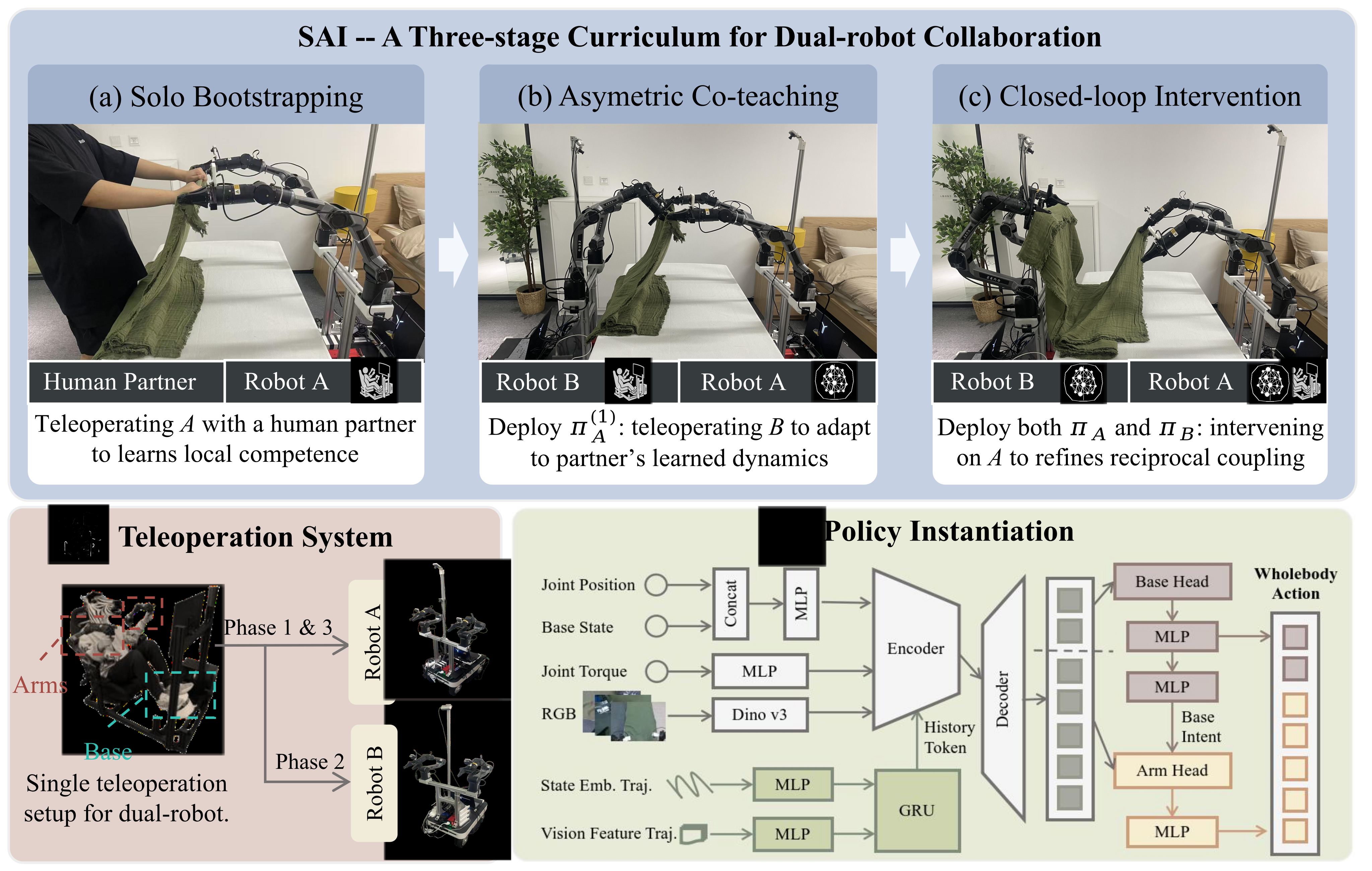
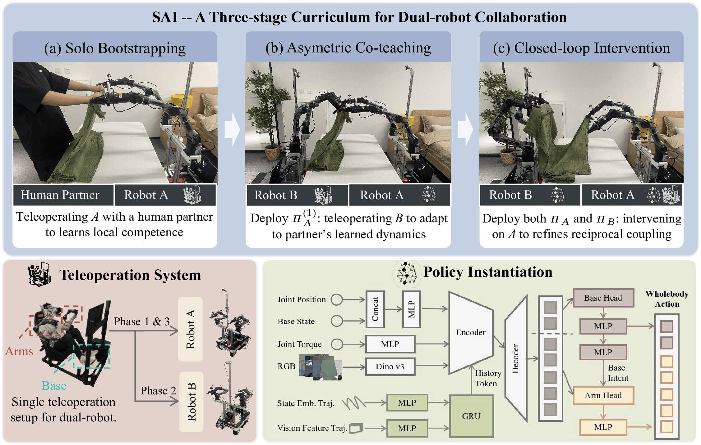
Single-Teleoperator Constraints: Standard dual-robot imitation learning assumes synchronized joint demonstrations, where both robots are controlled and recorded as one coordinated trajectory. This can require multiple teleoperation channels, calibrated interfaces, and precise temporal alignment between operators. We instead impose a single-teleoperator constraint: only one robot can be directly teleoperated at a time through one hardware interface. Under this constraint, supervision is decomposed into three asymmetric datasets: teleoperate Robot A with a compliant human or passive partner; teleoperate Robot B while the learned Robot-A policy is deployed; intervene on Robot A during closed-loop dual-robot deployment. The superscript in indicates that Robot B demonstrations are collected under the partner distribution induced by the learned Robot-A policy. The central question is whether these sequential, asymmetric datasets are sufficient to learn coupled decentralized policies that approach the cooperative behavior normally obtained from synchronized joint demonstrations.
4 Sequential Asymmetric Imitation
The data sequence is unilateralA demonstrations, teleoperatedB against learnedA, then correctiveA interventions in joint deployment. The partner changes from compliant external support to a frozen learned robot and finally a closed-loop robot pair. Equations 2–3 retain the exact curriculum and aggregation. The proposal is principally about which states/partner behaviors are supervised, with a particular history-based ACT implementation used for most experiments.

Original selectable mathematical display
Equation 2
| (2) |
Original mathematical definitions, policy details and evaluation protocol
Here, contains unilateral demonstrations for Robot A, contains Robot-B demonstrations collected while Robot A executes its learned policy, and contains corrective Robot-A interventions collected during joint deployment. Each robot acts from its own local history, including recent images, proprioception, and previous actions. The policies do not receive privileged partner state, explicit communication, or centralized coordination signals.
4.1 Stage 1: Bootstrapping Robot A
A human or passive partner supports the shared object while one operator teleoperatesA. Behavioral cloning learns nominal grasping, pulling and placement. Offline partner-region augmentation changes human appearance to discourage visual shortcuts. This establishes competence under supported conditions, not autonomous reciprocal coordination. The quality and coverage of these source demonstrations remain prerequisites.
Original mathematical definitions, policy details and evaluation protocol
Because the Stage-1 partner is human but the deployment partner is Robot B, a policy trained directly on these demonstrations may overfit to human-specific appearance and occlusion patterns. We therefore apply partner-masking augmentation to frames in which the supporting partner is visible: the partner region is replaced with randomized appearance perturbations, such as color jitter, blur, noise, or texture changes, with details in Appendix B. This encourages Robot A to focus on task-relevant object state rather than the visual identity of the supporting partner. Robot A is trained by behavioral cloning on the augmented demonstrations, producing the initial policy . This policy can perform the task with external support, but it has not yet learned to coordinate with an autonomous robot partner.
4.2 Stage 2: Training Robot B Against Deployed Robot A
The trainedA policy is frozen and deployed while the operator teleoperatesB. B learns againstA's actual timing, residual errors and motion profile. Bounded speed/action/timing/initial-state variation broadens exposure. The paper describes the types of variation but does not give complete quantitative distributions for all of them. This stage makesB partner-aware;A still carries its original human-support distribution mismatch.
Original mathematical definitions, policy details and evaluation protocol
The second stage freezes and deploys it on Robot A. A single operator then teleoperates Robot B while interacting with the deployed Robot-A policy. This produces , where Robot B observes the partner behavior it will face at test time.
Original mathematical definitions, policy details and evaluation protocol
During data collection, Robot A is executed with bounded deployment variation, such as speed scaling, action noise, timing offsets, or perturbed initial object states. These variations expose Robot B to realistic partner deviations and encourage waiting, yielding, recovery, and resumption behaviors. Robot B is then trained by behavioral cloning on the teleoperated actions, producing . This stage is asymmetric: Robot B is not trained against an ideal partner or a manually synchronized human partner, but against the actual learned behavior of Robot A. As a result, Robot B learns to compensate for Robot A’s timing, motion profile, and residual errors.
4.3 Stage 3: DAgger-Style Intervention Fine-Tuning
Both policies are deployed and the operator correctsA near coordination failures. Corrections are aggregated with nominalA replay and upweighted; optional action-dimension masks train only explicitly corrected components. Safety overrides onB during collection are not training labels. This is DAgger-style targeted correction, not exhaustive expert labeling of every learner state. Stage 3 adds about 30% of the baseline dataset size; complete per-task data counts and intervention-weight settings are not reported, so the comparison does not fully isolate curriculum order from added supervision.
Original mathematical definitions, policy details and evaluation protocol
To correct these failures, we deploy and together and collect sparse human interventions on Robot A. The intervention process is DAgger-style: the learned policies induce the closed-loop states, and the operator provides corrective labels only near states where coordination begins to fail. Each intervention records the current Robot-A history and the corrective action supplied by the operator. The resulting intervention dataset is aggregated with the original Robot-A demonstrations to fine-tune Robot A:

Original selectable mathematical display
Equation 3
| (3) |
4.4 Policy Instantiation
The frozen DINOv3 backbone supplies multi-view features. A 30-step history is logarithmically sampled to 12 frames and encoded by a one-layer GRU. The ACT decoder first predicts 3 base commands, then 14 arm/gripper commands conditioned on that base intent. This supports coherent whole-body action chunks. Coordination gains are evaluated with the same architecture across curriculum baselines, while architectural ablations separately measure particular failure modes.
Original mathematical definitions, policy details and evaluation protocol
To provide temporal context for coordination decisions, we maintain a history window of steps and select 12 frames using logarithmic temporal sampling. Multi-view visual features and full-body state features are fused and encoded by a single-layer GRU, whose final hidden state forms the history token. The ACT decoder then predicts a whole-body action chunk with a cascaded head: a base-action MLP first predicts , corresponding to , and an arm-action MLP then predicts conditioned on both the decoder query and the predicted base action. This architecture improves local execution reliability by encouraging base-arm consistency and preserving temporal context. However, the partner-responsive behavior comes from the SAI curriculum itself: each robot learns from progressively more realistic partner behavior, rather than from explicit communication, privileged partner state, or a centralized coordination loss.
5 Experimental Results
Four evaluation questions cover task success, response to partner delay, history/cascade ablations and ACT-versus-diffusion compatibility. RGB,17-dimensional proprioception and arm torque provide observations; no explicit inter-robot message channel is used. Success counts completed rollouts. PhaseSync counts predefined synchronized checkpoints, and Yield/Wait counts appropriate responses to partner-contingent opportunities. Events within one rollout are correlated, and their larger denominators do not create additional independent robot trials.
5.1 Q1: Does SAI improve collaboration across real-world tasks? Yes!
Each task/method has 30 rollouts. SAI success is 53.3%bed-throw,66.7%tablecloth,70.0%laundry and 56.7%painting, versus 23.3%,43.3%,50.0%and 33.3% for independent imitation. The two-stage partner-conditioned baseline lies between them. Full SAI further improves yielding to 68.3/70.0/71.7/68.9%. Table 1 retains every value and process metric; these gains are descriptive results on the evaluated tasks, with no reported training-seed intervals or general multi-robot guarantee.
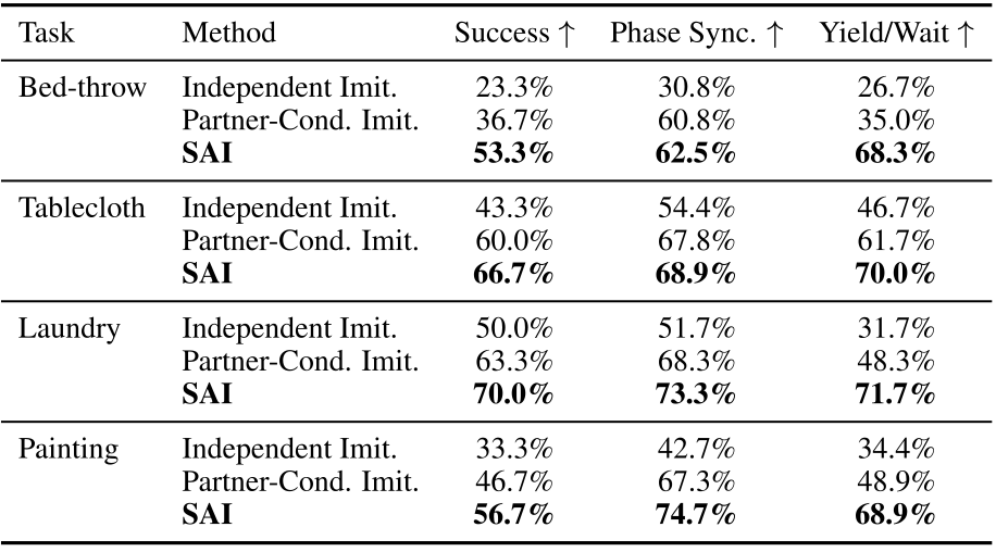
Accessible original table, complete values and event definitions
| Task | Method | Success | Phase Sync. | Yield/Wait |
| Bed-throw | Independent Imit. | 23.3% | 30.8% | 26.7% |
| Partner-Cond. Imit. | 36.7% | 60.8% | 35.0% | |
| SAI | 53.3% | 62.5% | 68.3% | |
| Tablecloth | Independent Imit. | 43.3% | 54.4% | 46.7% |
| Partner-Cond. Imit. | 60.0% | 67.8% | 61.7% | |
| SAI | 66.7% | 68.9% | 70.0% | |
| Laundry | Independent Imit. | 50.0% | 51.7% | 31.7% |
| Partner-Cond. Imit. | 63.3% | 68.3% | 48.3% | |
| SAI | 70.0% | 73.3% | 71.7% | |
| Painting | Independent Imit. | 33.3% | 42.7% | 34.4% |
| Partner-Cond. Imit. | 46.7% | 67.3% | 48.9% | |
| SAI | 56.7% | 74.7% | 68.9% |
5.2 Q2: Does SAI induce yielding under partner delay? Yes!
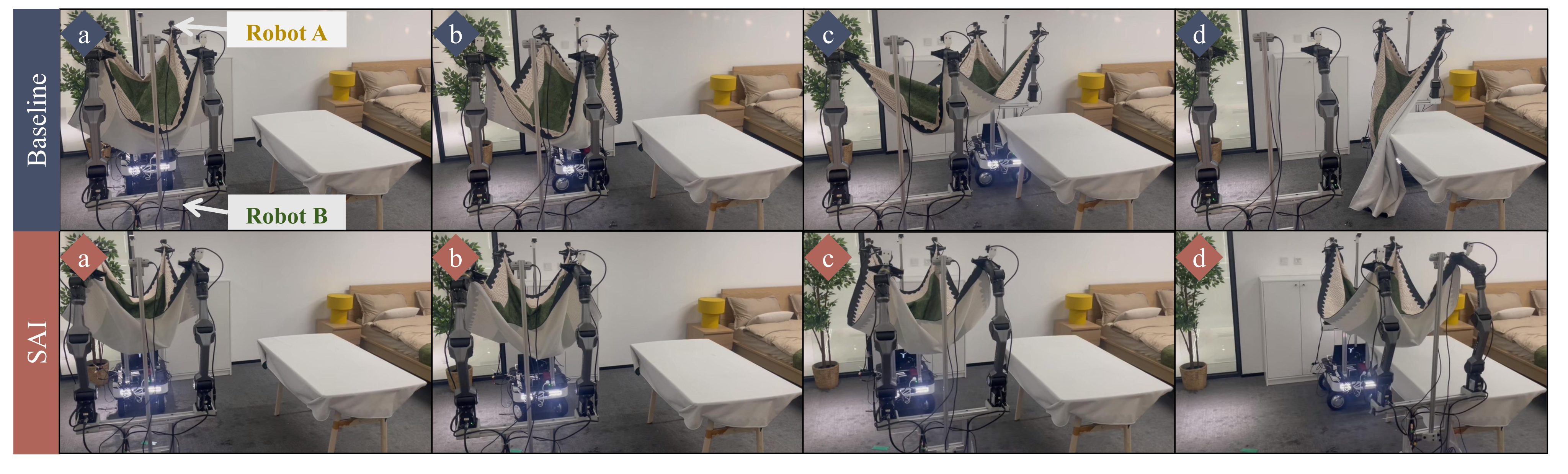
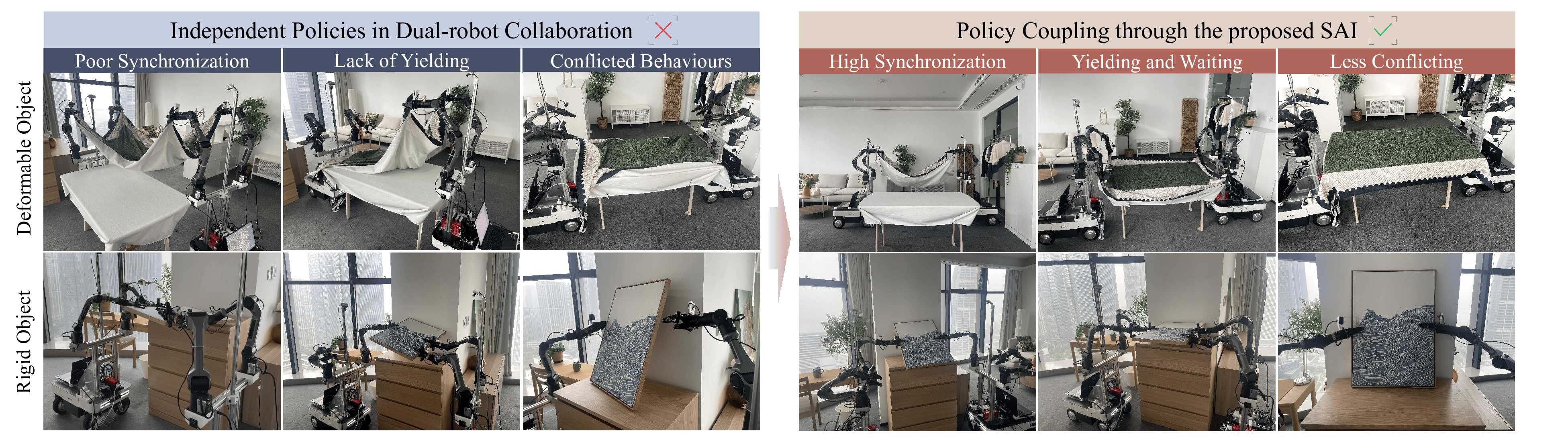
In Tablecloth Spreading, an operator pausesB during joint deployment. The illustrated independent policy keeps pulling, whileSAI slows, waits and resumes. Figure 4 retains all before/after panels. This is a controlled qualitative delay illustration accompanying aggregate Yield/Wait results. The paper does not specify the pause duration, number of dedicated delay trials or a separate delay-response success denominator, so the snapshots should not be converted into a new quantitative benchmark.
5.3 Q3: Do history and cascading components in the policy improve reliability? Yes!
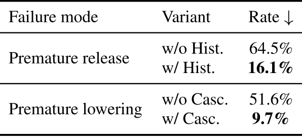
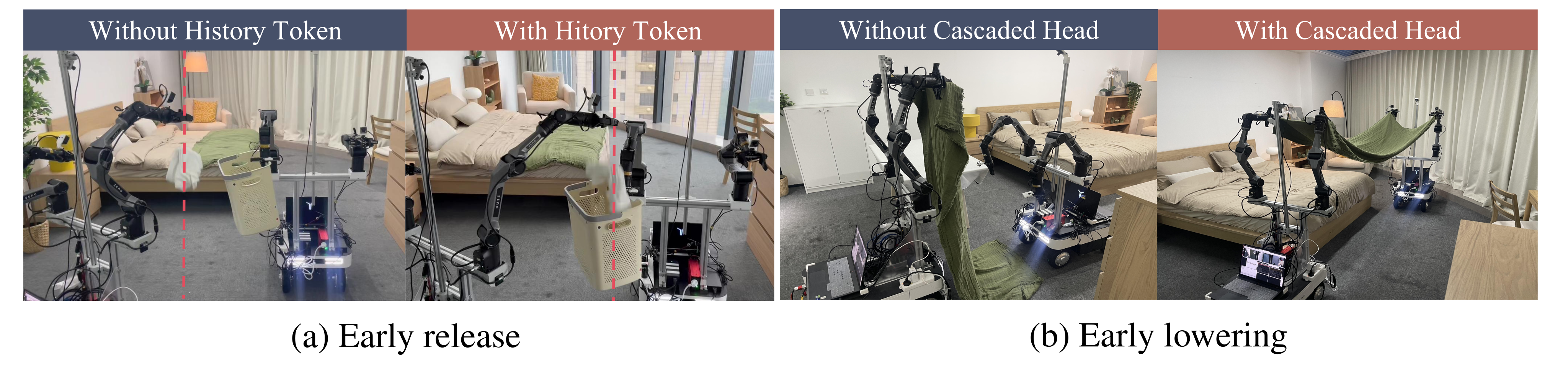
History reduces premature release from 64.5%to 16.1%; the cascaded head reduces premature lowering from 51.6%to 9.7%. AppendixC clarifies 31 targeted high-risk rollout segments per condition, rather than full-task trials from the beginning. These are 20/31 versus 5/31 and 16/31 versus 3/31 after rounding. They support reliability at the tested transitions. Since the curriculum baselines already share these components, the ablations address a different question from the full coordination comparison.
Accessible original table, complete values and event definitions
| Failure mode | Variant | Rate |
| Premature release | w/o Hist. | 64.5% |
| w/ Hist. | 16.1% | |
| Premature lowering | w/o Casc. | 51.6% |
| w/ Casc. | 9.7% |
5.4 Q4: Is SAI agnostic to specific imitation-learning backbones? Yes!
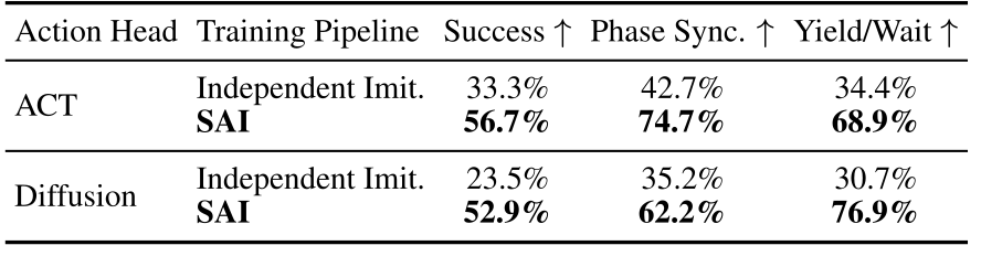
On Painting Transport, ACT success rises 33.3→56.7% with 30 rollouts/condition; Diffusion Policy rises 23.5→52.9% with 34. This supports compatibility with two tested backbones. The original Diffusion event metrics are retained, but AppendixC's stated shared checkpoint/opportunity definitions do not reconcile 35.2/62.2%phase and 30.7/76.9%yield with straightforward integer event totals from 34 rollouts. The paper does not provide an alternative aggregation or exclusions, so exact Q 4 event counts cannot be reconstructed from the stated protocol.
6 Conclusions and Limitations
The staged partner curriculum improves the reported four-task outcomes and qualitative response to a paused partner. It requires useful standalone primitives, observable partner progress and failures correctable by one robot at a time. Simultaneous two-robot corrections fall outside theA-centric design. Stage 3 coverage remains limited; more correction may help rare failures but can encourage unnecessary waiting. No formal stability, collision-clearance or out-of-distribution safety guarantee is established.
Original project figures and demonstration video
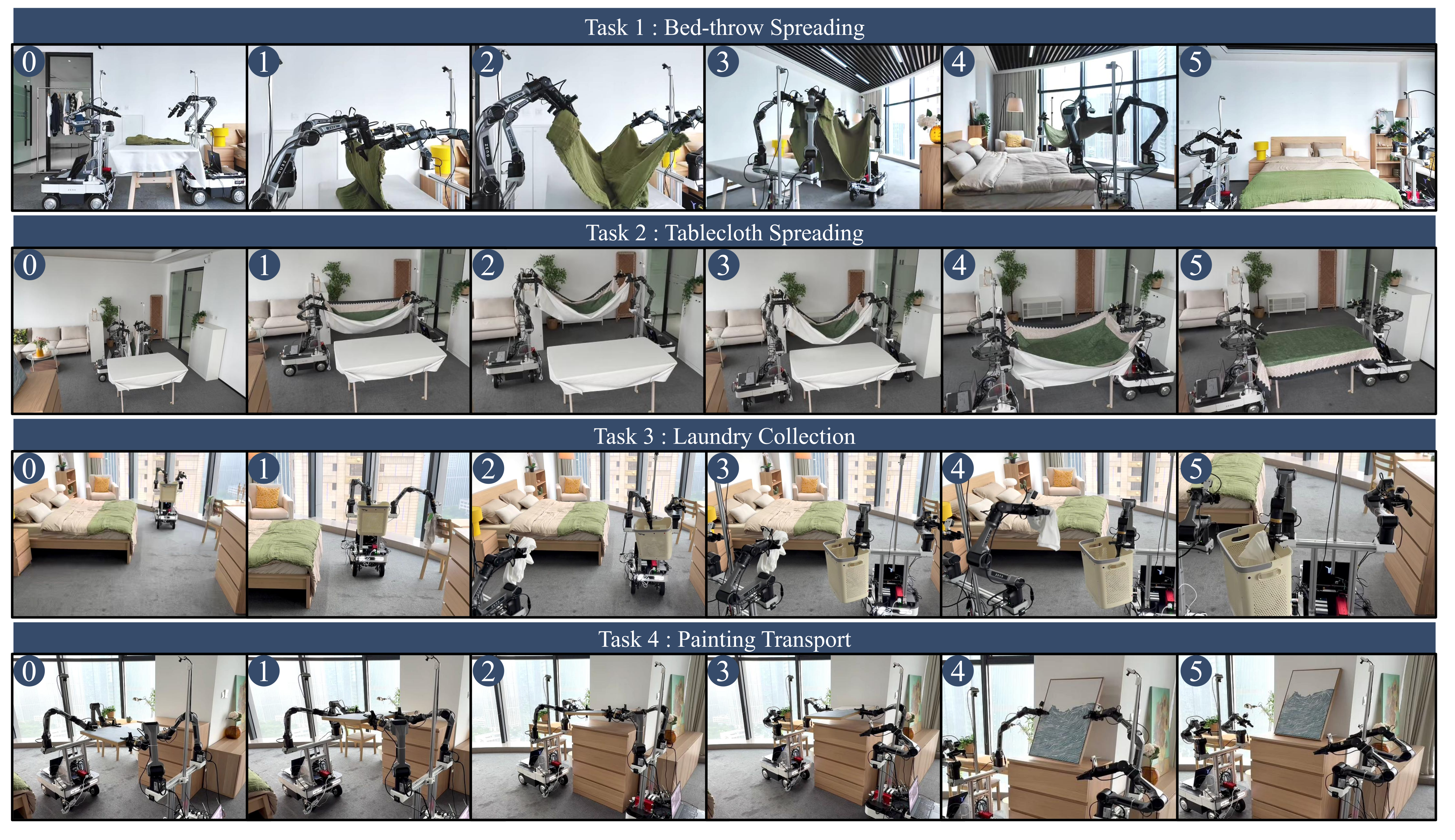
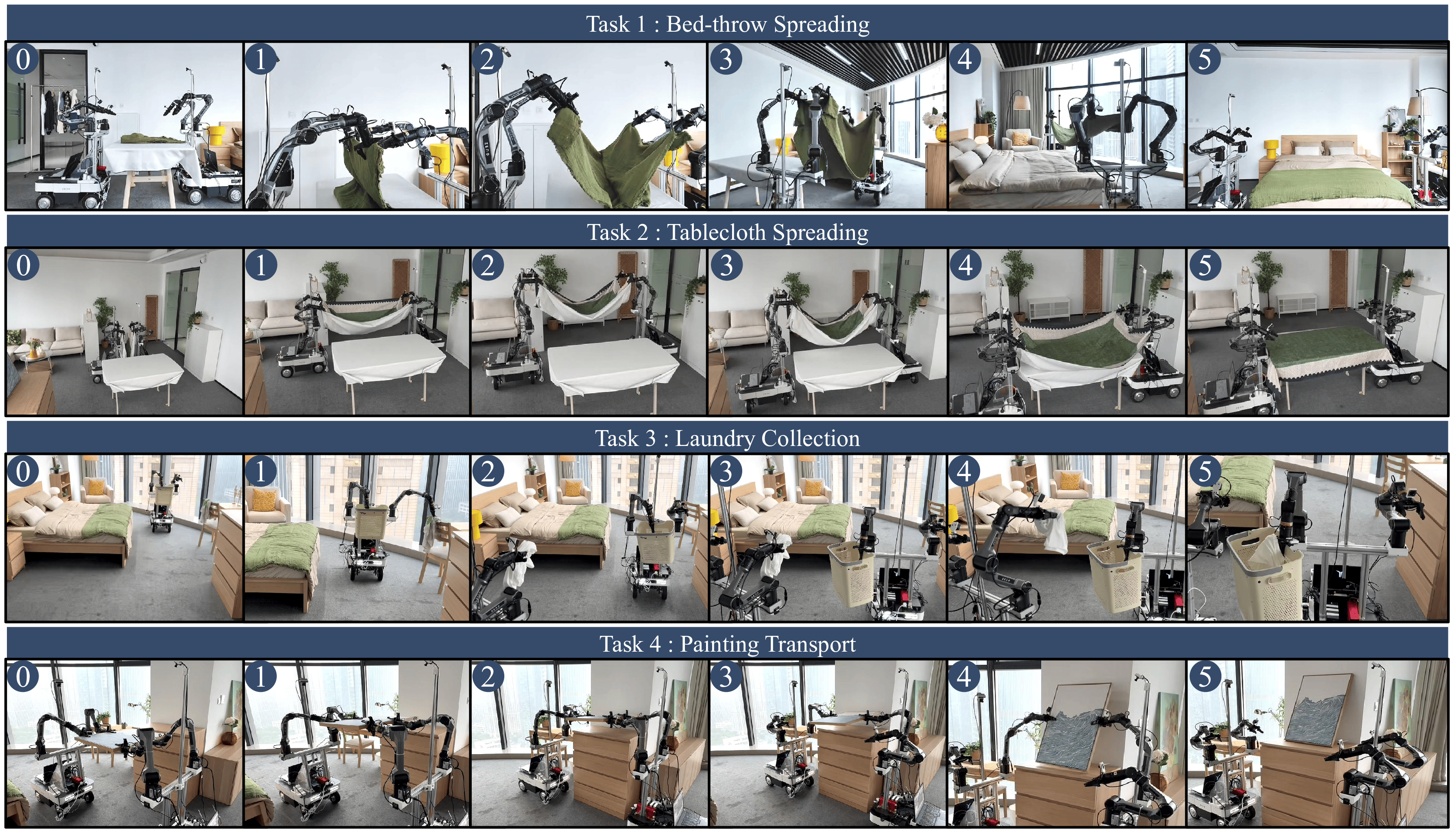
The three original project figures are preserved locally with unchanged source bytes and source URLs. The official demonstration video remains linked on YouTube; it is not described as a local recording. These illustrations complement the paper's six complete figures. Montage frames and repeated video views are not additional independent evaluation trials.
Appendix A Implementation Details and Reproducibility
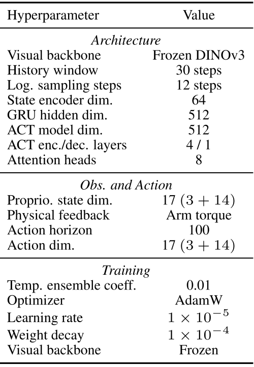
The implementation appendix supplies architecture, sensor/action spaces and training settings. These details define what 'decentralized' and 'local observation' mean in the experiment. All original notation and the complete hyperparameter table remain alongside the shortened notes. Hardware torque and a shared external camera contribute interaction information without an explicit communication protocol.
A.1 Network Architecture Details
Frozen DINOv3 ViT-Base features receive a 1×1 projection and 2 Dsinusoidal positions. Twelve log-spaced frames from a 30-step window fuse multi-view visual features with 64-dimensional state latents. A single-layer 512-unitGRU yields the history token, with padding masks for unavailable frames. Two-layer MLP heads predict base then arm/gripper actions. Base conditioning encourages coherent execution but does not encode an explicit partner-action model.
Original mathematical definitions, policy details and evaluation protocol
Visual Encoder. We use a frozen DINOv3 (ViT-Base) backbone [33] to extract spatial features from RGB observations, including the shared top camera and egocentric wrist cameras. The feature maps are projected with a convolution and flattened into image tokens before entering the transformer encoder. Two-dimensional sinusoidal positional embeddings are added to preserve spatial information.
Original mathematical definitions, policy details and evaluation protocol
History encoder. To provide temporal context for long-horizon decisions, we maintain a history window of steps. For efficiency, we select 12 historical frames with logarithmic temporal sampling, using denser samples near the current timestep and sparser samples further in the past. For each sampled timestep, multi-view visual features are pooled and projected, while the full-body state is encoded by an MLP into a 64-dimensional latent. The visual and state latents are concatenated, passed through a fusion MLP, and encoded by a single-layer GRU with hidden dimension 512. Padding masks are used when historical frames are unavailable. The final GRU hidden state is used as the history token .
Original mathematical definitions, policy details and evaluation protocol
Cascaded whole-body action head. The ACT decoder outputs action-query embeddings. Instead of predicting all action dimensions with a single flat head, we use a cascaded structure. A 2-layer MLP first predicts the mobile-base action , corresponding to . The predicted base intent is then concatenated with the decoder query and passed to a second 2-layer MLP to predict the arm-gripper action . This factorization conditions arm and gripper commands on the imminent base motion and improves whole-body action consistency.
A.2 State and Action Space Definitions
Each observation includes top/wrist RGB,17-dimensional base-plus-arm/gripper proprioception and measured arm torque. Each action is 17-dimensional:3 base velocities(vx,vy,ω)plus 14 arm/gripper commands. Action chunks have horizon 100 and exponential temporal ensembling coefficient 0.01. A shared top camera can observe partner/object progress; absence of messaging should not be confused with absence of shared scene information or physical feedback.
Accessible original table, complete values and event definitions
| Hyperparameter | Value |
| Architecture | |
| Visual backbone | Frozen DINOv3 |
| History window | 30 steps |
| Log. sampling steps | 12 steps |
| State encoder dim. | 64 |
| GRU hidden dim. | 512 |
| ACT model dim. | 512 |
| ACT enc./dec. layers | 4 / 1 |
| Attention heads | 8 |
| Obs. and Action | |
| Proprio. state dim. | 17 |
| Physical feedback | Arm torque |
| Action horizon | 100 |
| Action dim. | 17 |
| Training | |
| Temp. ensemble coeff. | 0.01 |
| Optimizer | AdamW |
| Learning rate | |
| Weight decay | |
| Visual backbone | Frozen |
Original mathematical definitions, policy details and evaluation protocol
The policy predicts an action chunk of horizon . Each action step has dimension , consisting of a 3D base command and a 14D arm-gripper command. During execution, overlapping chunks are combined with exponential temporal ensembling using coefficient .
A.3 Training Details and Hyperparameters
AdamW uses learning rate 10⁻⁵ and weight decay 10⁻⁴. Table 4 retains model dimension 512,4 encoder/1 decoder layers and 8 attention heads. Stage 3 binary loss masks select corrected chunk components to avoid overwriting untouched actions. Nominal replay helps preserve prior competence. Quantitative intervention weighting, full training schedules and complete demonstration counts are not specified, limiting exact reproduction of the data-budget comparison.
Original mathematical definitions, policy details and evaluation protocol
All policies are trained with AdamW. During Stage 3, interventions may correct only part of the action space, such as stopping the base while maintaining arm posture. We therefore use binary action-loss masks for intervention samples, so gradients are applied only to explicitly corrected action dimensions. This prevents sparse corrective labels from overwriting nominal behavior in unaffected dimensions.
Appendix B Partner Masking and Randomization
Offline partner segmentation, dilation and masked appearance replacement aim to reduceA's reliance on human-specific visual identity. The process is used during training/data loading, not policy inference. Source transformations preserve the surrounding workspace while changing pixels in the detected human region. The paper does not separately quantify the contribution of each augmentation or segmentation errors.
Offline partner-region detection.
An off-the-shelf instance segmenter estimates the human region, and Equation 4 dilates it with a circular kernel to cover boundaries/shadows. The model choice and numerical dilation radius are not specified here. This masks human appearance rather than removing every implicit interaction cue. The complete original mathematical definitions remain available, including the distinction between estimated and dilated masks.
Original mathematical definitions, policy details and evaluation protocol
For each raw observation , we use an off-the-shelf instance segmentation model to obtain a binary human-region mask . To cover boundary artifacts, thin uncovered regions, and nearby shadows, we dilate the mask with a circular structuring element:
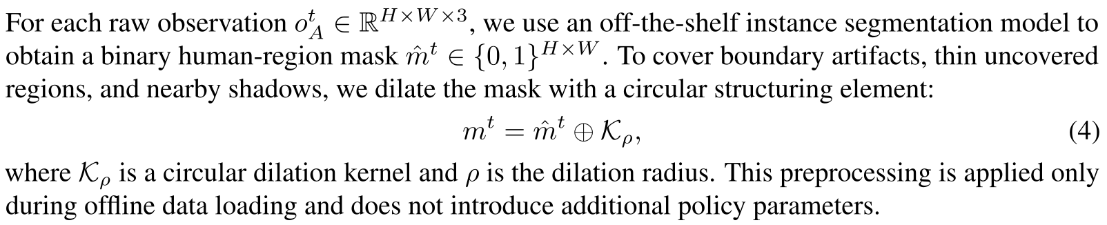
Original selectable mathematical display
Equation 4
| (4) |
Original mathematical definitions, policy details and evaluation protocol
where is a circular dilation kernel and is the dilation radius. This preprocessing is applied only during offline data loading and does not introduce additional policy parameters.
Partner-region randomization.
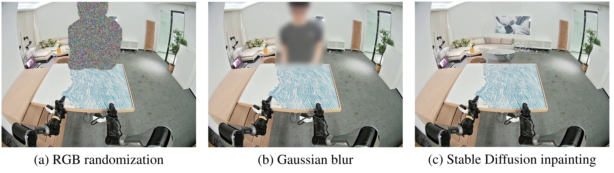
Equation 5 blends unchanged scene pixels with a random replacement inside the partner mask. The alternatives are independent RGB noise, strong Gaussian blur and mask-guided Stable Diffusion inpainting. Figure 6 preserves all three examples and labels. Generated fills may change local cues, so the method regularizes appearance rather than certifying semantic invariance. These operations add no inference-time segmentation requirement in the described pipeline.
Original mathematical definitions, policy details and evaluation protocol
Given the dilated mask , we construct an augmented observation:

Original selectable mathematical display
Equation 5
| (5) |
Original mathematical definitions, policy details and evaluation protocol
where is a stochastic replacement operator applied only inside the masked partner region. The goal is not to remove all interaction evidence, but to make human-specific appearance cues unreliable during policy learning. This encourages the policy to rely less on the visual identity of the human partner and more on task-relevant scene cues, such as object geometry, deformation, contact progress, and workspace configuration. During offline training-time data loading, randomly samples one of the following partner-region transformations:
Appendix C Evaluation Protocol and Rollout Statistics
AppendixC specifies rollout counts, event denominators and ordered checkpoint definitions. It is essential for interpreting the main percentages. Thirty-rollout task success,31 targeted ablation segments and 34 Diffusion-policy rollouts represent different experiment populations. All seven tables, including the complete long checkpoint table, remain readable and selectable.
General protocol.
Success is rollout-level; PhaseSync and Yield/Wait are event-level descriptive percentages from the same rollouts. Later checkpoints not reached after failure count as failed. The authors say thresholds/stage definitions are fixed across methods, but numerical timing tolerances are not supplied. Event counts do not justify treating checkpoints within a rollout as statistically independent samples.

Accessible original table, complete values and event definitions
| Experiment | Evaluation scope | Conditions | Rollouts / condition |
| Q1 | Per-task comparison | 4 tasks 3 methods | 30 |
| Q3 | Policy ablations | Failure-specific variants | 31 |
| Q4 | Backbone compatibility | Diffusion on Painting | 34 |
Q1: per-task evaluation.
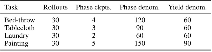
Q 1 uses 30 rollouts for every task/method. Phase denominators are 120 bed-throw,90 tablecloth,60 laundry and 150 painting; yielding denominators are 60/60/60/90. Table 1 percentages are compatible with integer counts at these denominators. This reconstructability supports reading the reported values correctly, while leaving training-repeat variability and annotator/protocol details unquantified.
Accessible original table, complete values and event definitions
| Task | Rollouts | Phase ckpts. | Phase denom. | Yield denom. |
| Bed-throw | 30 | 4 | 120 | 60 |
| Tablecloth | 30 | 3 | 90 | 60 |
| Laundry | 30 | 2 | 60 | 60 |
| Painting | 30 | 5 | 150 | 90 |
Phase Sync.
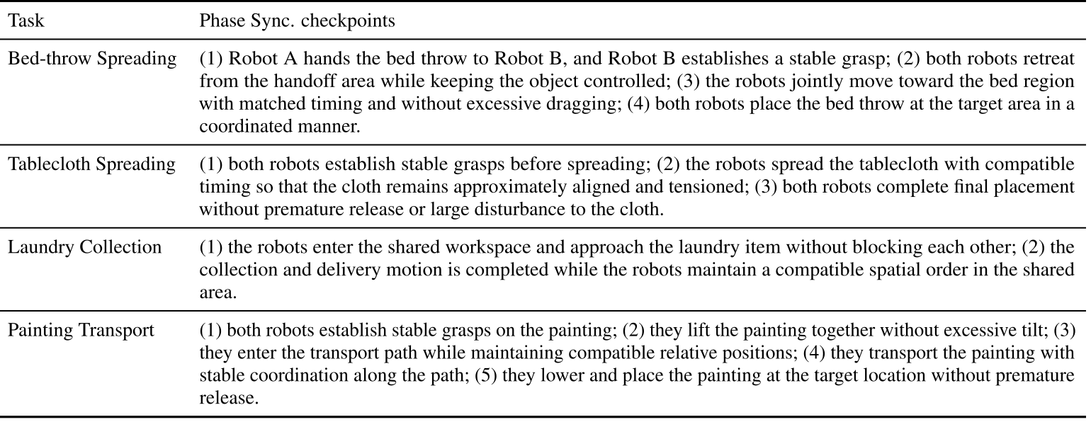
Ordered checkpoints cover handoff/retreat/transport/placement for bed-throw; coordinated grasp/spread/place for tablecloth; workspace approach and delivery for laundry; and grasp/lift/enter/transport/place for painting. Table 7 retains the full definitions, including absence of disruptive interaction. Synchronization requires both timing agreement and controlled object behavior. The paper states task-specific fixed tolerances without listing their numerical thresholds.
Original mathematical definitions, policy details and evaluation protocol
For each task, we divide the cooperative process into ordered event stages. These stages define the checkpoints used to compute Phase Sync.. The Phase Sync. checkpoints for each task are listed in Table 7. For a task with checkpoints per rollout and evaluated rollouts, the denominator is . The numerator is the number of checkpoints for which both robots reach and complete the corresponding stage within the predefined timing tolerance and without causing a task-disrupting interaction. Thus, Phase Sync. is computed as the percentage of synchronized checkpoints over all evaluated checkpoints. If a rollout fails before reaching a later stage, all unreached checkpoints are counted as failed. Stage definitions and timing thresholds are fixed per task and kept identical across all evaluated methods. For example, Painting Transport has five checkpoints per rollout; with 30 rollouts, the Phase Sync. denominator is .
Yield/Wait.
A yielding opportunity is correct if a robot slows, waits, yields, adjusts pose or resumes only when its partner is ready. These are behavioral events in a shared task, not a separate set of whole-rollout successes. Table 6 gives fixed per-task totals across methods. Exact opportunity scheduling and the temporal boundary for judging a response are not fully detailed.
Accessible original table, complete values and event definitions
| Task | Phase Sync. checkpoints |
| Bed-throw Spreading | (1) Robot A hands the bed throw to Robot B, and Robot B establishes a stable grasp; (2) both robots retreat from the handoff area while keeping the object controlled; (3) the robots jointly move toward the bed region with matched timing and without excessive dragging; (4) both robots place the bed throw at the target area in a coordinated manner. |
| Tablecloth Spreading | (1) both robots establish stable grasps before spreading; (2) the robots spread the tablecloth with compatible timing so that the cloth remains approximately aligned and tensioned; (3) both robots complete final placement without premature release or large disturbance to the cloth. |
| Laundry Collection | (1) the robots enter the shared workspace and approach the laundry item without blocking each other; (2) the collection and delivery motion is completed while the robots maintain a compatible spatial order in the shared area. |
| Painting Transport | (1) both robots establish stable grasps on the painting; (2) they lift the painting together without excessive tilt; (3) they enter the transport path while maintaining compatible relative positions; (4) they transport the painting with stable coordination along the path; (5) they lower and place the painting at the target location without premature release. |
Q3: policy-component ablations.
Q 3 uses 31 targeted segments near high-risk release/lowering transitions. Laundry release tests whether the garment is dropped before a valid receiving state. Lowering tests whether the arm descends before the base finishes transport. These local failure rates explain the architectural ablation numbers but should not be merged with Q 1's 30 full-rollout success rates.
Q4: backbone compatibility.
Q 4 uses Painting Transport, with ACT reusing 30 rollout conditions and Diffusion Policy using 34. The source states the same event definitions. With 5 phase checkpoints per rollout,170 events would not round to the printed 35.2/62.2%; with 3 yield opportunities,102 events would not produce 30.7/76.9%. Unreported exclusions, weighting or repeated runs could account for this. The edition preserves all source values and flags the missing aggregation detail rather than inventing counts or inferring a code fault.