At a glance
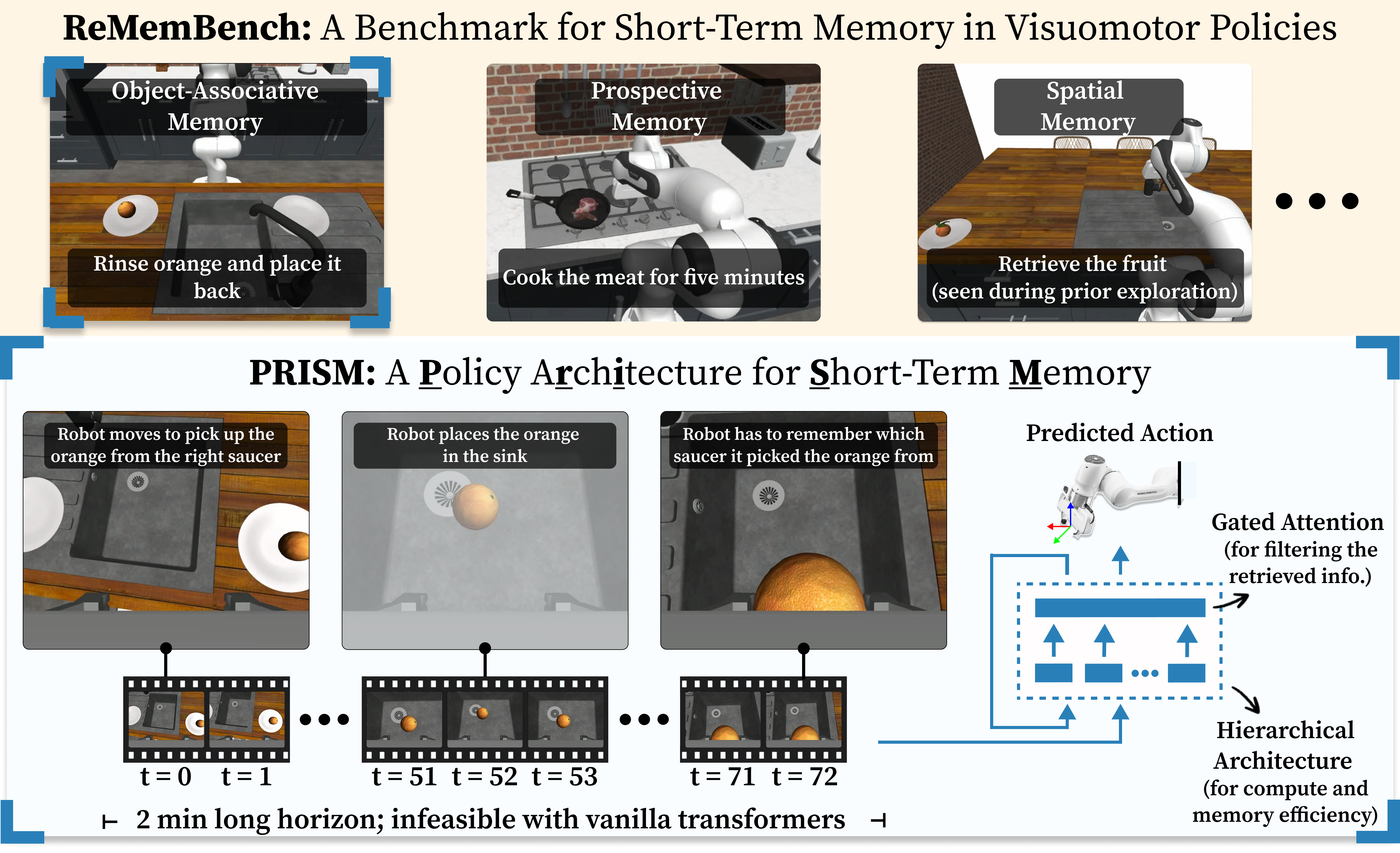
PRISM adds input-conditioned attention gates and hierarchical token compression to a causal visuomotor policy. It uses recent sensory and action history to address partial observability while reducing the cost of long contexts. ReMemBench supplies eight household tasks covering four memory categories. The main matched baseline comparison uses four of those tasks: PRISM averages 41% success there, versus 36% for the strongest baseline, while its all-eight-task average is 32%. A physical wash-and-return task reaches 30% versus 15% for the past-token-prediction baseline. These gains leave substantial failure rates.
I Introduction
A current image cannot reveal where an occluded object was placed, which container an object came from, or how long a stove has been on. Simply extending a transformer’s context adds irrelevant inputs and expensive visual tokens. PRISM addresses these problems through feature-wise gating after attention and compression before global temporal attention. Its memory is a sliding window of recent interaction, not a persistent record spanning different days or episodes.
| Benchmark | Domain | Episode Length | Short-term memory categories | |||
| Spatial | Prospective | Object-Associative | Object-Set | |||
| ALFRED [20] | Manipulation | 1000 | ✓ | ✗ | ✗ | ✗ |
| Habitat MultiON [21] | Navigation | 2500 | ✓ | ✗ | ✗ | ✗ |
| FindingDory [22] | Navigation + manipulation | 3500 | ✓ | ✓ | ✗ | ✗ |
| Memory Maze [17] | Navigation | 4000 | ✓ | ✗ | ✗ | ✗ |
| Memory Gym [23] | Synthetic gridworlds | -1 | ✓ | ✗ | ✓ | ✗ |
| POPGym [24] | Synthetic games | 1024 | ✓ | ✗ | ✓ | ✓ |
| MemoryBench [18] | Manipulation | 12 | ✓ | ✗ | ✓ | ✗ |
| Mikasa-Robo [25] | Manipulation | 180 | ✓ | ✓ | ✗ | ✗ |
| RoboMME [26] | Manipulation | 1300 | ✓ | ✗ | ✓ | ✓ |
| ReMemBench | Navigation + manipulation | 2500 | ✓ | ✓ | ✓ | ✓ |
II Related Work
Related work spans recurrent memory, attention architectures, robot policies, and benchmarks that require recall.
Short-Term Memory in Machine Learning
Recurrent networks retain history in a fixed hidden state; transformers expose stored tokens directly but increase context costs. Gating, sparse or hierarchical attention, and segment recurrence offer ways to control information flow and resource use. PRISM adapts gating and hierarchical attention to closed-loop imitation learning.
Short-Term Memory in Visuomotor Policies
Robot policies often condition on only recent frames. Alternatives store spatial states, select keyframes, compress trajectories, or add auxiliary reconstruction objectives. Past-Token Prediction [15] is an important comparison. PRISM changes the policy backbone and uses the standard behavior-cloning objective, without a separate memory-reconstruction loss.
Memory Benchmarks
Benchmarks differ in whether memory is explicitly necessary or merely helpful alongside perception and exploration. ReMemBench organizes longer navigation-and-manipulation episodes around spatial, prospective, object-associative, and object-set memory. Its teleoperated dataset targets imitation learning, while other suites emphasize shorter episodes or other learning settings. These differences complicate direct cross-benchmark claims.
III PRISM : A P olicy A r ch i tecture for S hort-Term M emory
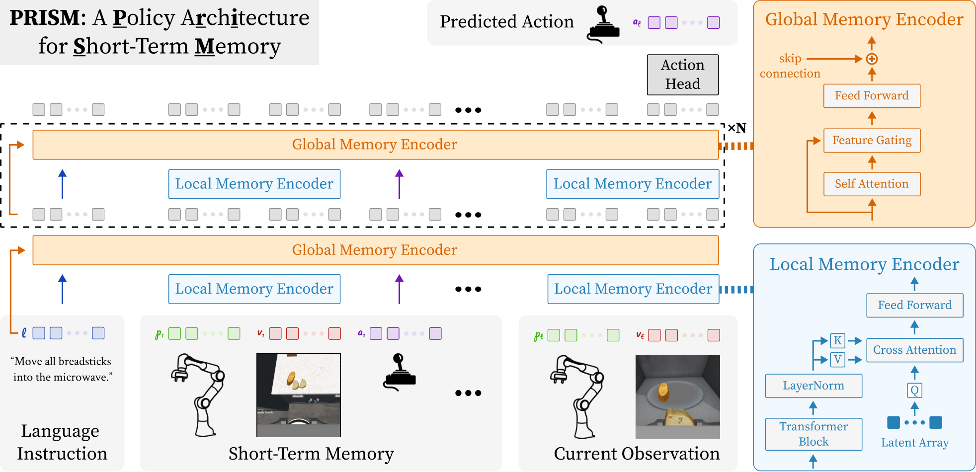
PRISM combines a conventional history-conditioned policy formulation with two architectural changes: filtering retrieved features and compressing the tokens used for global memory.
III-A Formulation, Background, and Challenges
The policy learns from instructed expert trajectories under partial observability and predicts action chunks from recent observations and actions.
Problem Formulation
Each demonstration pairs a language instruction with observations and expert actions. The policy conditions on the available interaction history rather than treating the current observation as a fully observable state.
Equation
Training Objective
Behavior cloning maximizes the likelihood of demonstrated actions. The action head predicts a chunk of future actions, preserving the original loss and policy equations below.
Equation
Evaluation
At inference, the instruction is a static prefix and new observation/action tokens enter the context. Once the configured memory budget is reached, the oldest interaction steps are discarded. Evaluation varies object identities and placements within the specified tasks.
Model Architecture
Image, proprioceptive, past-action, and language encoders create causally ordered tokens with positional information. A transformer processes the truncated history, and an action head reads an observation hidden state to parameterize the next action chunk. The language encoder is pretrained.
Equations 1
| (1) |
Challenges
Long contexts create two distinct difficulties: irrelevant history can correlate with actions in the training data, and storing/attending to many visual tokens increases compute and memory. The following components address information flow and resource use respectively.
III-B Selecting Relevant Features
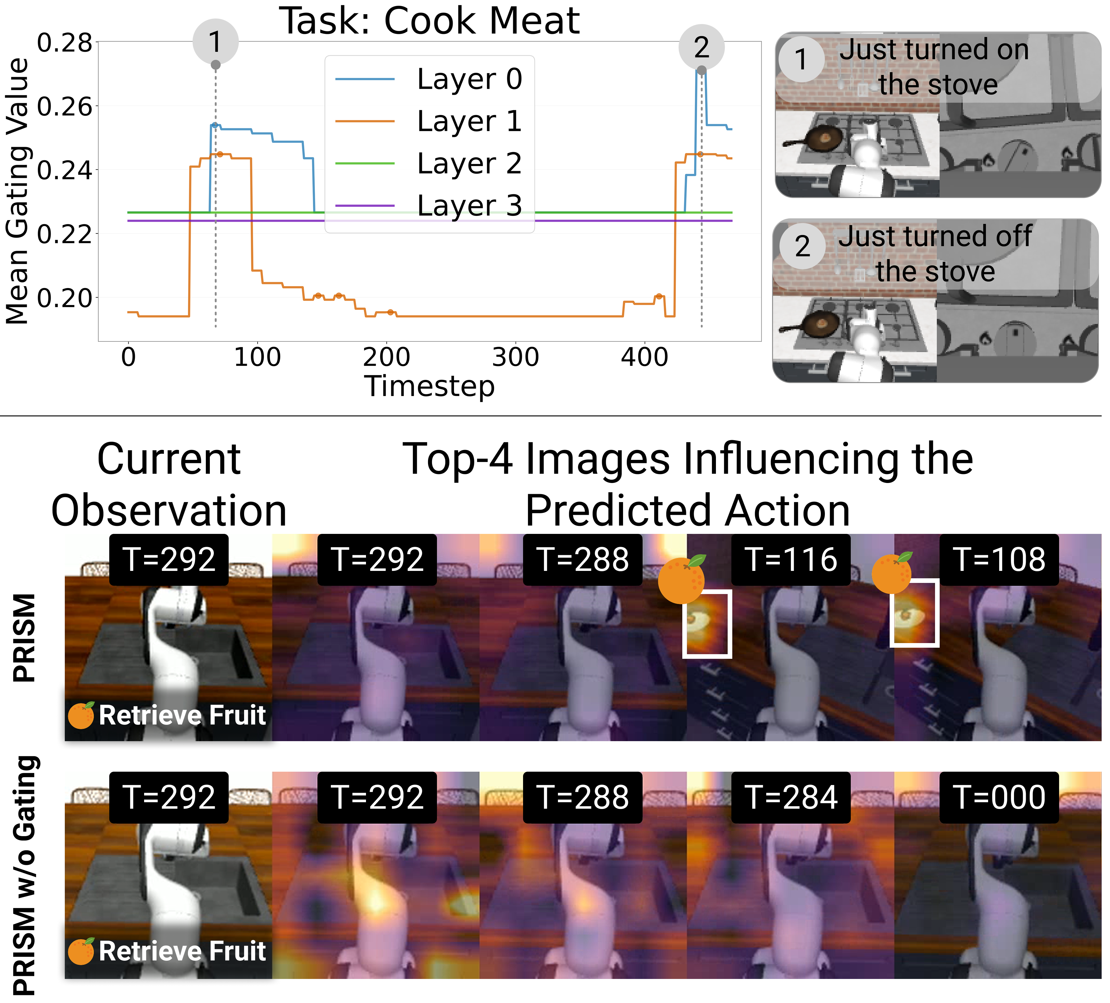
Following gated attention [12], a sigmoid multilayer perceptron maps current input features to an element-wise gate on the attention output. Gating occurs after value aggregation, before the output projection and residual connection. It can suppress retrieved feature dimensions without removing old frames or directly selecting a subset of stored timesteps.
The ablations support useful filtering, although the architecture alone does not guarantee removal of spurious correlations. The feature-conditioned gate is more expressive than a single learned scalar per layer.
Equations
III-C Reducing Memory and Compute Footprint
A local encoder summarizes the current sensory tokens, and global attention integrates these compact summaries over time. Global information is then broadcast back and combined with original local features through a residual skip, preserving detailed current inputs. The hierarchy reduces the length of global attention and the cached history. Its theoretical savings concern the global component; practical end-to-end gains also depend on local encoding, visual processing, and implementation overhead.
Equations
Summary.
Together, gating controls the retrieved representation and hierarchy makes longer contexts affordable. Both are trained as part of the imitation policy without an auxiliary memory objective.
IV ReMemBench: A Benchmark for Short-Term Memory in Visuomotor Policies
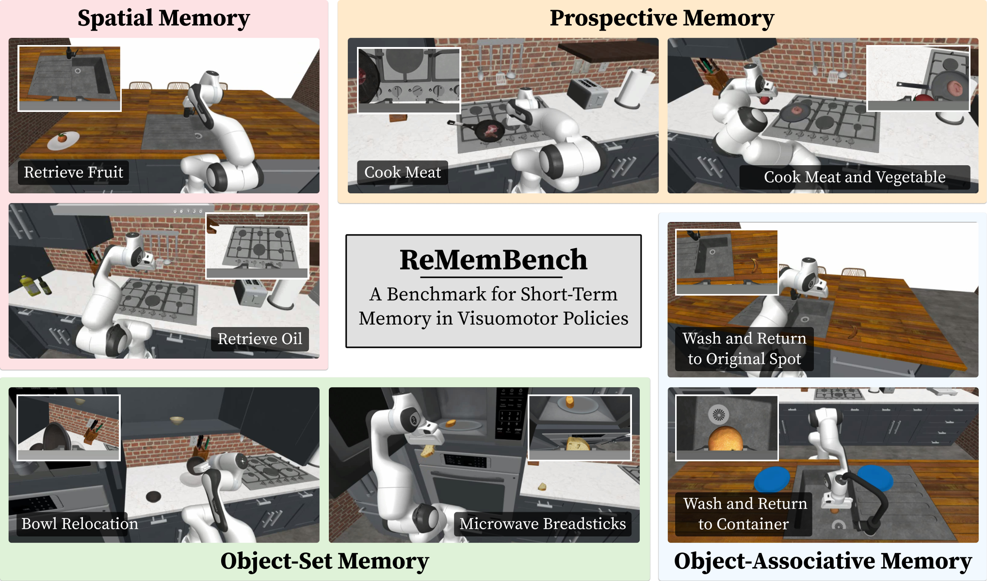
ReMemBench extends RoboCasa [16] with eight tasks and fifty teleoperated demonstrations per task. Spatial tasks retrieve a fruit or oil bottle whose location must be remembered. Prospective tasks turn a stove off after a delay or time the addition of a second ingredient. Associative tasks wash an object and return it to its original container or countertop position. Set-memory tasks move all breadsticks into a microwave or all bowls, excluding distractor plates, into a cabinet.
Object identities, placements, counts, or timing requirements vary across trials. The suite combines recall with difficult perception and control, so failure does not by itself isolate a defective memory mechanism.
V Experiments
The principal baseline table evaluates four representative tasks with twenty trials per task across three seeds. PRISM averages 0.41 ± 0.04, versus 0.36 ± 0.02 for the scene-memory transformer, 0.28 for past-token prediction, 0.25 for Mamba, and 0.12 for the long short-term memory model. PRISM’s strongest relative gain is prospective timing; the scene-memory transformer is better on the spatial and object-set tasks. The separate all-eight-task PRISM row is 0.32 ± 0.08 and has no corresponding all-eight-task baseline rows.
On a physical wash-and-return adaptation trained from one hundred demonstrations, success is 30% for PRISM, 15% for past-token prediction, and 0% without memory. The source does not specify the number of physical test trials. This is evidence from one task, with most attempts still failing.
On four RoboCasa atomic tasks, memory raises success from 0.32 to 0.43. On the five listed LIBERO suites, the average rises from 0.77 to 0.89. Published baseline numbers are taken from earlier works rather than a fully matched training comparison. The RoboCasa table labels the GR00T baseline N1-2B, whereas the abstract/introduction call it N1-3B; the reported 0.32 score is retained without resolving that naming discrepancy. Although no large robot-policy pretraining is used, PRISM does use pretrained visual and language encoders.
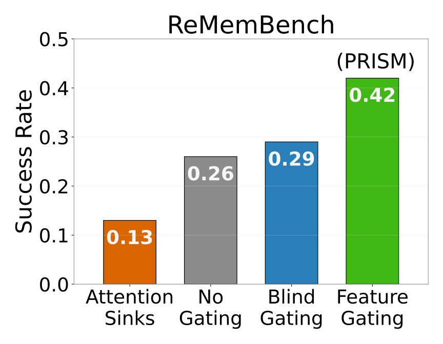
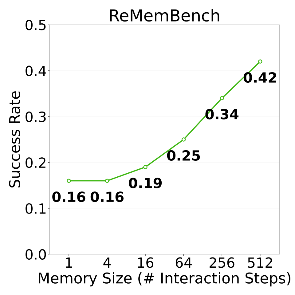
Increasing the memory window from one to 512 steps raises the plotted success from 0.16 to 0.42. Feature-wise gating obtains 0.42, versus 0.29 for blind gating, 0.26 without gating, and 0.13 with attention sinks. These ablation values should not be substituted for the main table’s separately reported 0.41 result.
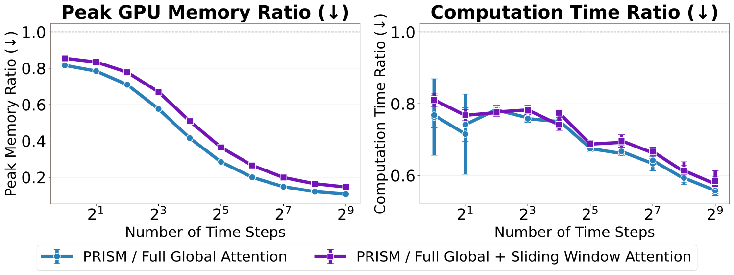
At 512 steps, the reported peak-memory and compute-time ratios are 0.20 and 0.60 relative to the compared full-attention designs. The appendix measures parameter-normalized repeated unit blocks, so these are architecture microbenchmarks, not whole-policy robot latency or throughput measurements.

| Method | Success Rate |
| GR00T-N1-2B | 0.32 |
| Diffusion Policy | 0.26 |
| PRISM (no memory) | 0.32 |
| PRISM () | 0.43 |
VI Limitations and Conclusion
Success remains low on the full memory benchmark, and perception, control, and recall can all limit performance. The method stores a recent window within an episode; persistent long-term memory and retrieval across a robot’s lifetime remain future work. Larger video-based memory pretraining is also proposed rather than evaluated. The results support a useful architecture and challenging benchmark, while not establishing dominance on every task or memory setting.
VII Acknowledgements
The authors acknowledge feedback and resources from the Robotics and AI Institute and Texas Advanced Computing Center, along with federal research support. Two authors conducted much of the work during institute internships.
VIII Appendix
The appendices examine attention sharpness and dropping, gating controls, another benchmark, compression, complexity, and implementation.
IX Effect of Attention Scale Factor (Sharpness)
On the Retrieve Fruit task, making attention very flat reduces success to 0.22 at scale 0.125, compared with 0.64 at scales 1 and 2. Sharper settings vary non-monotonically, with 0.54 at scale 4 and 0.62 at 8. This single-task sweep supports sensitivity to weak selectivity; it is not a benchmark-wide average or a guarantee that increasing sharpness improves performance.
X Effect of Attention Dropping
Dropping attention tokens with probability 0.1 raises average success from 0.45 to 0.49 with gating and from 0.26 to 0.39 without it. Gating remains helpful in both conditions. These appendix runs use a different reported baseline level from the main 0.41 table; the source does not fully reconcile the settings, so their values remain distinct.
| Method | Spatial | Prospective | Associative | Object-Set | Average |
| PRISM w/o Gating | 0.08 | 0.35 | 0.30 | 0.30 | 0.26 |
| PRISM w/o Gating (Attn Drop) | 0.44 | 0.80 | 0.10 | 0.20 | 0.39 |
| PRISM | 0.40 | 0.80 | 0.25 | 0.35 | 0.45 |
| PRISM (Attn Drop) | 0.60 | 0.64 | 0.30 | 0.40 | 0.49 |
XI Effect of Gating Module
A scalar gate and a feature-wise gate both include sigmoid nonlinearities and have similar parameter counts: 86 million versus 90 million. Feature-wise gating reaches 0.45 versus 0.28 for the scalar version. This narrows the explanation beyond simply adding any nonlinearity, though the capacity and architecture are not exactly identical.
| Method | Spatial | Prospective | Associative | Object-Set | Average |
| Blind Gating | 0.35 | 0.30 | 0.25 | 0.20 | 0.28 |
| Feature Gating (PRISM) | 0.40 | 0.80 | 0.25 | 0.35 | 0.45 |
XII Evaluation on Mikasa-Robo
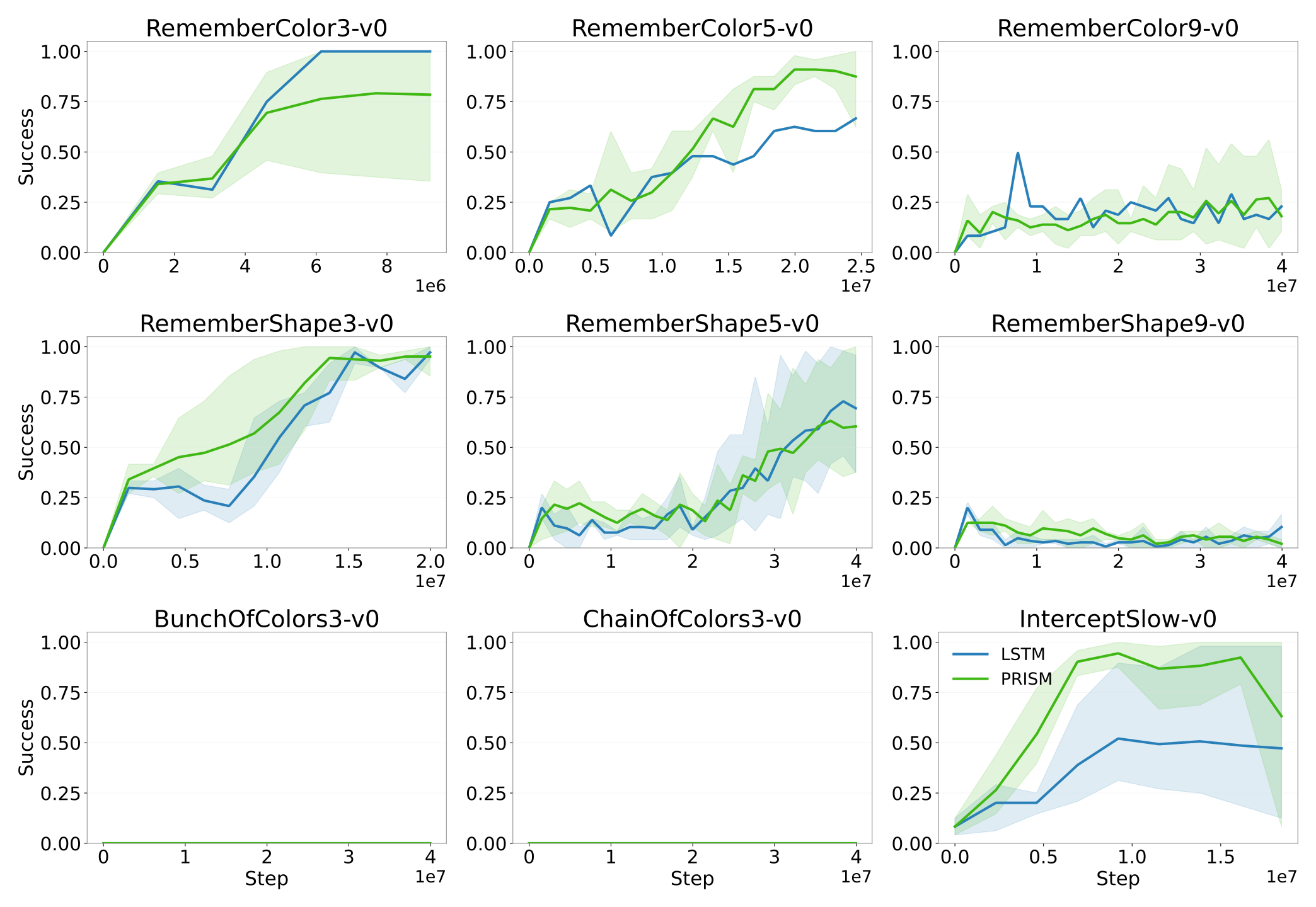
On Mikasa-Robo, PRISM improves some tasks but is comparable overall to the long short-term memory baselines. The authors attribute the difference from ReMemBench to shorter horizons, fewer distractors, and information concentrated in early frames. These are plausible explanations requiring further controlled study, rather than established causal findings.
XIII Analysis of the compression factor ( m )
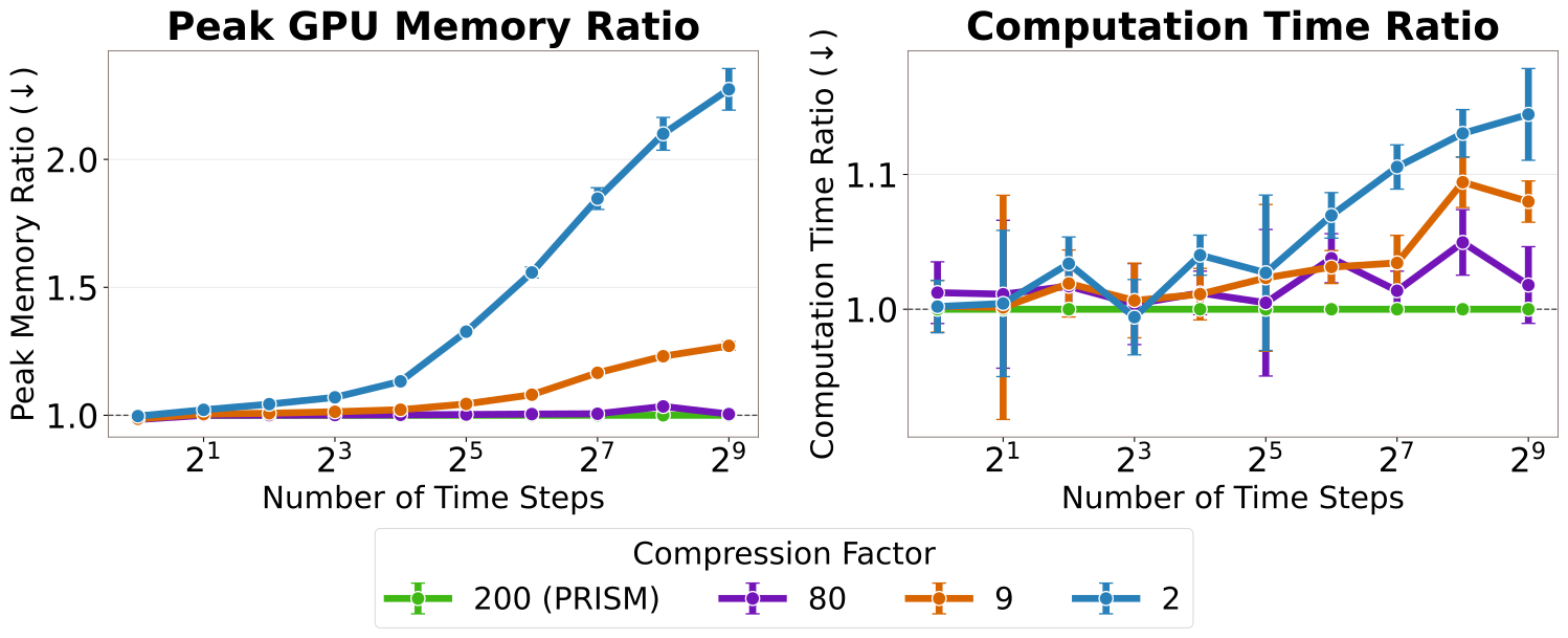
Compression factors near 2, 9, 80, and 200 yield average success of 0.31, 0.40, 0.41, and 0.45. The experiments share a 384 H100 GPU-hour budget; the less-compressed models complete fewer gradient steps, so the comparison mixes representation and optimization-budget effects. At 512 steps, the most compressed configuration uses 13% less compute and 56% less peak memory than the least compressed in the reported unit-block measurements.
| Compression () | Spatial | Prospective | Associative | Object-Set | Average |
| 0.30 | 0.40 | 0.28 | 0.24 | 0.31 | |
| 0.40 | 0.56 | 0.24 | 0.40 | 0.40 | |
| 0.40 | 0.60 | 0.24 | 0.40 | 0.41 | |
| (PRISM) | 0.40 | 0.80 | 0.25 | 0.35 | 0.45 |
XIV Memory and Compute Footprint
The complexity analysis separates local processing from attention over the compressed temporal sequence.
Training.
Training cost contains a local term linear in sequence length and a quadratic global term over the compressed tokens. Reducing the global sequence can save activations, but optimized attention implementations already reduce that memory cost, limiting realized savings relative to simple asymptotic estimates.
Equation
Evaluation.
At inference, compact summaries reduce the global key/value cache and the tokens attended to at each step by approximately the compression factor. This does not imply the same factor of improvement for the full policy, whose other components remain.
Baselines
The compute comparison runs one architecture block twenty times, records wall-clock duration and peak memory, and normalizes measurements by parameter count. Full global attention and a global-plus-sliding-window hybrid are the baselines. This protocol bounds interpretation of the efficiency plots.
XV Implementation Details
Implementation details specify the actual token compression, demonstration counts, and training budget.
PRISM Architecture Details
Two cameras supply 396 visual tokens, proprioception one, and the previous action one. The 397 sensory tokens compress to one summary, leaving two tokens per step and a factor of 199. The backbone follows a LLaMA-style transformer; the action head is a two-layer perceptron. Visual features come from frozen pretrained CrossMAE [63].
Data Collection
A human collects fifty space-mouse demonstrations per ReMemBench task and one hundred for the physical task. These are the imitation data used in the reported setups, separate from encoder pretraining.
| Config | Value |
| Optimizer | AdamW |
| Base learning rate | |
| Effective batch size | 256 |
| Weight decay | |
| Warmup epochs | |
| Total epochs | |
| Action prediction horizon | |
| Proprioception noise (std) | |
| Brightness augmentation | |
| Contrast augmentation | |
| Number of cameras |
Training Details
Training uses about 384 H100 GPU-hours for the eight ReMemBench tasks and 192 for four RoboCasa atomic tasks. The retained table specifies AdamW with learning rate 0.0005, batch size 256, 200 epochs, two warmup epochs, and a 32-step action horizon, along with image and proprioceptive augmentation.