Overview
This edition follows the complete twenty-four-page, 14 October 2026 v2, including both full system prompts, all seven traffic prompts and their generated programs, and the complete machine-learning appendix. The rules are the study’s modeling examples, not independently verified statements of traffic law.
At a glance
TraCS combines a frozen motion predictor with probabilistic traffic rules and a learned decision about whether to use them. It reweights six existing trajectory candidates without moving their points. On Argoverse 2, the three tested backbones obtain small average improvements in Brier-style prediction metrics and larger conditional gains in their highest-error scenarios. The result concerns forecasting and calibration; it does not establish safe closed-loop driving or recover a correct path missing from the candidate set.
1 Introduction
Motion predictors learn common traffic behavior but may exploit shortcuts or underrepresent uncommon road users. TraCS supplies a separate description of desired behavior, grounded in uncertain spatial relations, then learns when that description helps a particular predictor. Its three components are probabilistic rule construction, symbolic trajectory scoring and contextual trust gating.
The experiments attach this machinery to DeMo, Polaris and QCNet. Frozen prediction weights do not mean a training-free addition: a separate gate is fitted for each backbone, and the full gate accesses its penultimate representations.
2 Related Work
Motion Prediction in Ground Mobility.
Classical Bayesian tracking maintains uncertainty over state, whereas modern interaction-aware predictors learn multiple future paths from scene context. Language-based trajectory models and NeSyMoF offer other ways to add structured knowledge. TraCS keeps the original trajectory generator and changes only its candidate probabilities, so its scope and failure modes differ from generating or refining paths.
Neuro-Symbolic Representation and Reasoning.
ProbLog, DeepProbLog, NeurASP and neural-probabilistic ASP connect logic with uncertain or learned predicates. The paper uses the Resin reactive reasoning system to combine declarative rules with continuously updated spatial evidence. Exact reasoning is relative to the encoded program and probability model; it does not certify that the natural-language rule was faithfully translated.
Agentic Program Synthesis.
Earlier LLM-to-ASP work, LLASP and solver-assisted language models motivate a coding loop. Here a compiler checks syntax and an LLM judge critiques semantics before another attempt. These checks provide feedback, not a formal equivalence proof between the prompt and generated program.

3 Trajectory Compliance-Shaping for Motion Predictions
The pipeline samples uncertain map geometry, evaluates state and transition relations, encodes natural-language rules over those relations, scores each proposed trajectory, and combines symbolic and neural scores through a learned gate. Figure 1 retains the complete information flow.
3.1 Transitional Statistical Spatial Relations
Building on StaR Maps, the method repeatedly transforms uncertain feature geometry and evaluates a relation at a queried state. Binary relations become Bernoulli probabilities; real-valued relations such as distance are represented by fitted distributions. Transitional relations additionally depend on velocity and a time increment, so they can describe entering, crossing or following a feature.
This probabilistic grounding represents the selected geometric uncertainty model. Relations derived from common sampled geometry can be dependent; multiplying probabilistic facts requires the joint assumptions of the logic model, rather than following automatically from their separate marginals.
Equation 1
| (1) |
3.2 Agentic Traffic Regulation Modeling
The coding agent receives a fixed vocabulary of map features, motion relations and sensor quantities. It writes a Resin program, receives compiler and judge feedback, and iterates until acceptance or its budget is exhausted. The experiments conjoin the programs for all supplied constraints.
Appendix A retains the exact prompts and programs. The judge is explicitly allowed to accept approximate core logic when the vocabulary lacks details such as turn signals or pedestrian intent. Semantic acceptance is therefore weaker than complete real-world rule fidelity, and a syntactically valid program may still express a different boundary or agent scope.
3.3 Neuro-Symbolic Trajectory Scoring
Weighted model counting produces state-level compliance under the specified logic and probabilistic atoms. A trajectory score is the geometric mean of its sampled state scores, then normalized across candidates. This is a ranking score; it is not the joint probability that an entire trajectory remains compliant.
The log-linear fusion is equivalent to normalizing p_neural × p_symbolic^w. The uniform-reference term is common to every candidate and cancels in normalization. With w=0 the original distribution is recovered; with w=1 the distributions form a product. Uniform symbolic scores leave the predictor unchanged, but “comparably low” compliance must mean similar relative scores: merely making every absolute score small does not make their normalized scores uniform. Handling an all-zero score vector is not specified.
Equations 2–4
| (2) |
| (3) |
| (4) |
3.4 Model Alignment and Trust Gating
A trust network predicts when symbolic reweighting is useful from hand-crafted score/context features and optional backbone embeddings. Supervision searches a grid of 1,000 fusion weights for the lowest expected ADE on each training scene, then fits a soft binary-cross-entropy target.
Deployment thresholds the learned output into a binary gate: either full symbolic fusion or exact fallback to the neural probabilities. The threshold is selected per backbone on validation data. Thus the reported system does not continuously attenuate rules using the raw trust score, and the gate is an empirical forecast-quality decision rather than a safety certificate.
Equations 5–7
| (5) |
| (6) |
| (7) |
4 Experiments
Evaluation uses Argoverse 2, six proposals per focal agent, three frozen backbones and ten gate-training seeds. The AV2 validation split trains and validates the gate; the held-out test split contains 24,984 focal-agent scenarios.
Program compilation averages 21.04 seconds and 5,998 tokens. Reported inference is 1.86±0.29 Hz, while the final fusion operation alone runs at 6,060 Hz. The fast multiplication/normalization stage should not be mistaken for the complete reasoning pipeline’s rate.
4.1 Agentic Codification for TraCS
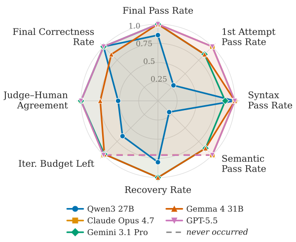
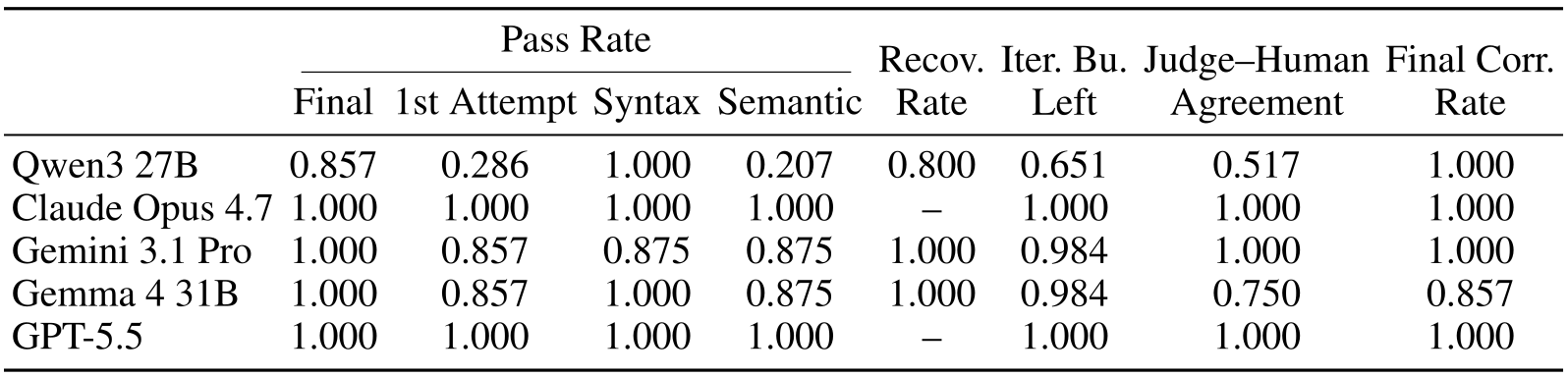
Figure 2 and Table 4 compare five language models on the seven supplied traffic-rule cases. Compiler syntax success, judge acceptance and final human correctness are separate outcomes. For example, Qwen3 27B has syntax pass rate 1.0 but semantic pass rate 0.207; Gemma 4 31B has final pass rate 1.0 but final correctness 0.857.
Claude Opus 4.7 and GPT-5.5 receive 1.0 on the reported first-attempt and final correctness measures. This small vocabulary-specific sample demonstrates variation in translation quality; it is not a broad validation of legal reasoning or unrestricted road scenarios.
Original selectable table
| bMinADE6 (↓) | bMinADE1 (↓) | bMinFDE1 (↓) | |||||
| Backbone | Mode | Base | +TraCS | Base | +TraCS | Base | +TraCS |
| DeMo | Overall | 1.3185 | 1.3172 (0.1%) | 2.1900 | 2.1842 (0.3%) | 4.5940 | 4.5887 (0.1%) |
| Bus | 1.5107 | 1.5073 (0.2%) | 2.5072 | 2.4661 (1.6%) | 4.8436 | 4.7718 (1.5%) | |
| Cyclist | 1.3356 | 1.3305 (0.4%) | 1.9574 | 1.9493 (0.4%) | 3.7022 | 3.7014 (0.0%) | |
| Motorcyclist | 1.5473 | 1.5450 (0.1%) | 2.6472 | 2.6258 (0.8%) | 5.3926 | 5.3562 (0.7%) | |
| Pedestrian | 1.0041 | 1.0016 (0.2%) | 1.2375 | 1.2121 (2.1%) | 1.9985 | 1.9690 (1.5%) | |
| Vehicle | 1.3318 | 1.3307 (0.1%) | 2.2468 | 2.2440 (0.1%) | 4.7807 | 4.7800 (0.0%) | |
| Polaris | Overall | 1.2713 | 1.2696 (0.1%) | 2.1131 | 2.1075 (0.3%) | 4.4036 | 4.4043 (0.0%) |
| Bus | 1.4685 | 1.4680 (0.0%) | 2.4212 | 2.4074 (0.6%) | 4.6466 | 4.6806 (0.7%) | |
| Cyclist | 1.2977 | 1.2957 (0.2%) | 1.8204 | 1.8187 (0.1%) | 3.3874 | 3.3959 (0.3%) | |
| Motorcyclist | 1.4241 | 1.4172 (0.5%) | 2.3567 | 2.3432 (0.6%) | 4.7648 | 4.7657 (0.0%) | |
| Pedestrian | 0.9565 | 0.9534 (0.3%) | 1.1383 | 1.1218 (1.4%) | 1.8903 | 1.8736 (0.9%) | |
| Vehicle | 1.2846 | 1.2830 (0.1%) | 2.1740 | 2.1695 (0.2%) | 4.5890 | 4.5895 (0.0%) | |
| QCNet | Overall | 1.2477 | 1.2476 (0.0%) | 2.0693 | 2.0643 (0.2%) | 4.6856 | 4.6765 (0.2%) |
| Bus | 1.4119 | 1.4147 (0.2%) | 2.3010 | 2.2628 (1.7%) | 4.7257 | 4.6768 (1.0%) | |
| Cyclist | 1.2634 | 1.2657 (0.2%) | 1.7129 | 1.7020 (0.6%) | 3.4995 | 3.4858 (0.4%) | |
| Motorcyclist | 1.3736 | 1.3747 (0.1%) | 2.2972 | 2.2786 (0.8%) | 5.2616 | 5.2346 (0.5%) | |
| Pedestrian | 0.9522 | 0.9522 (0.0%) | 1.0634 | 1.0586 (0.5%) | 1.8676 | 1.8621 (0.3%) | |
| Vehicle | 1.2612 | 1.2610 (0.0%) | 2.1367 | 2.1332 (0.2%) | 4.9029 | 4.8953 (0.2%) | |
4.2 Motion Forecasting on TraCS
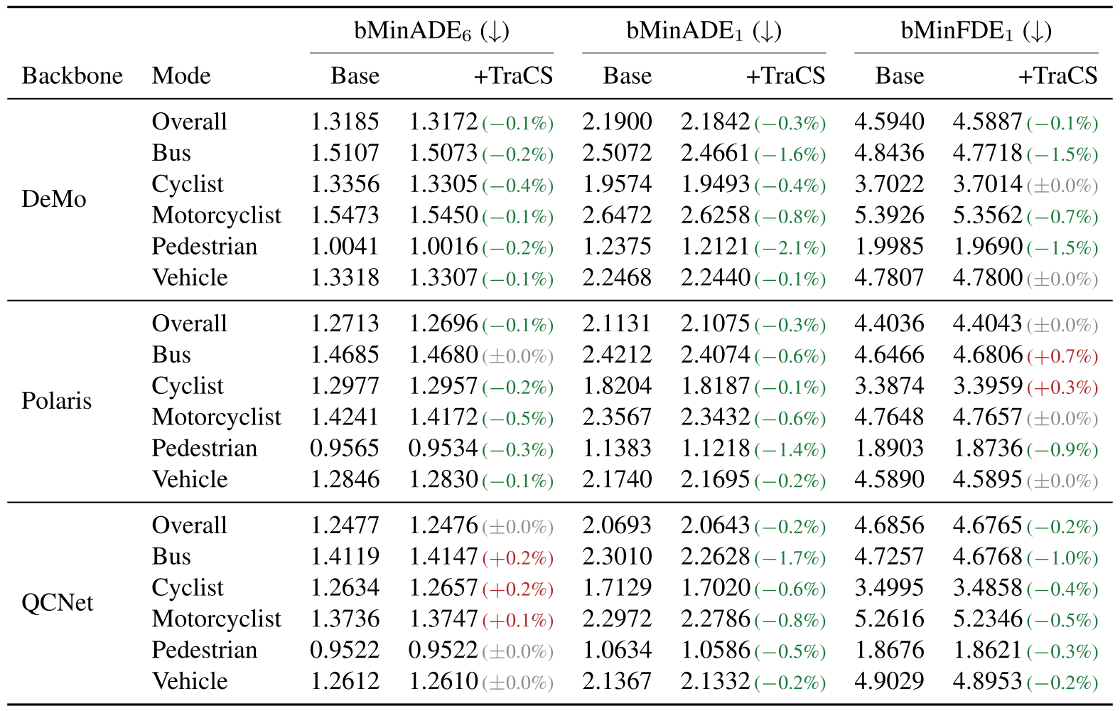
All eighteen backbone-by-class bMinADE₁ cells in Table 1 improve. The prose and Table 2 report population changes of −0.0039, −0.0061 and −0.0047 for DeMo, Polaris and QCNet; equal-class-weight improvements are −0.0145, −0.0100 and −0.0173. The authors report paired tests and hierarchical bootstrap intervals excluding zero.
There is an unresolved numerical difference: subtracting the displayed overall bMinADE₁ values in Table 1 gives −0.0058, −0.0056 and −0.0050, rather than the prose/Table 2 changes. Both original tables are retained. Improvements also depend on the metric: Polaris bus/cyclist bMinFDE₁ worsens, and several QCNet bMinADE₆ entries worsen. Omitted deterministic K=1 metrics are described as within ±0.3% of baseline. Reweighting cannot improve the geometry of the fixed candidate set.
4.3 TraCS-based Tail-Risk Mitigation
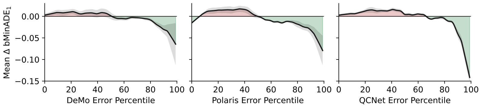
Figure 3 conditions on each backbone’s prediction-error percentile. The lowest 60–70% of scenes change little on average, while the worst decile improves by −0.044, −0.054 and −0.088 bMinADE₁, reported as 8.9–18.7 times the population mean gain.
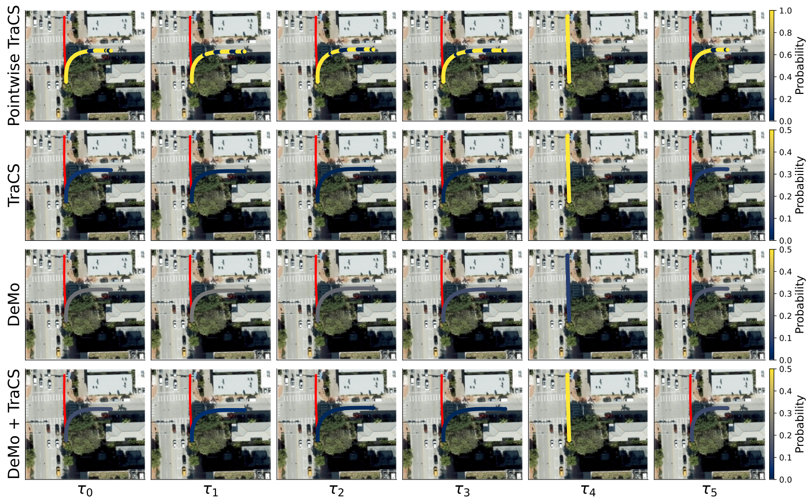
These are smoothed conditional average forecast changes, not a worst-case safety bound or a guarantee for each high-error scene. Figure 4 illustrates one DeMo bus case: symbolic evidence moves the correct straight candidate τ₄ from lowest to highest probability. No planner rollout or collision-rate evaluation establishes the downstream driving benefit.
4.4 Impact per Mode of Mobility
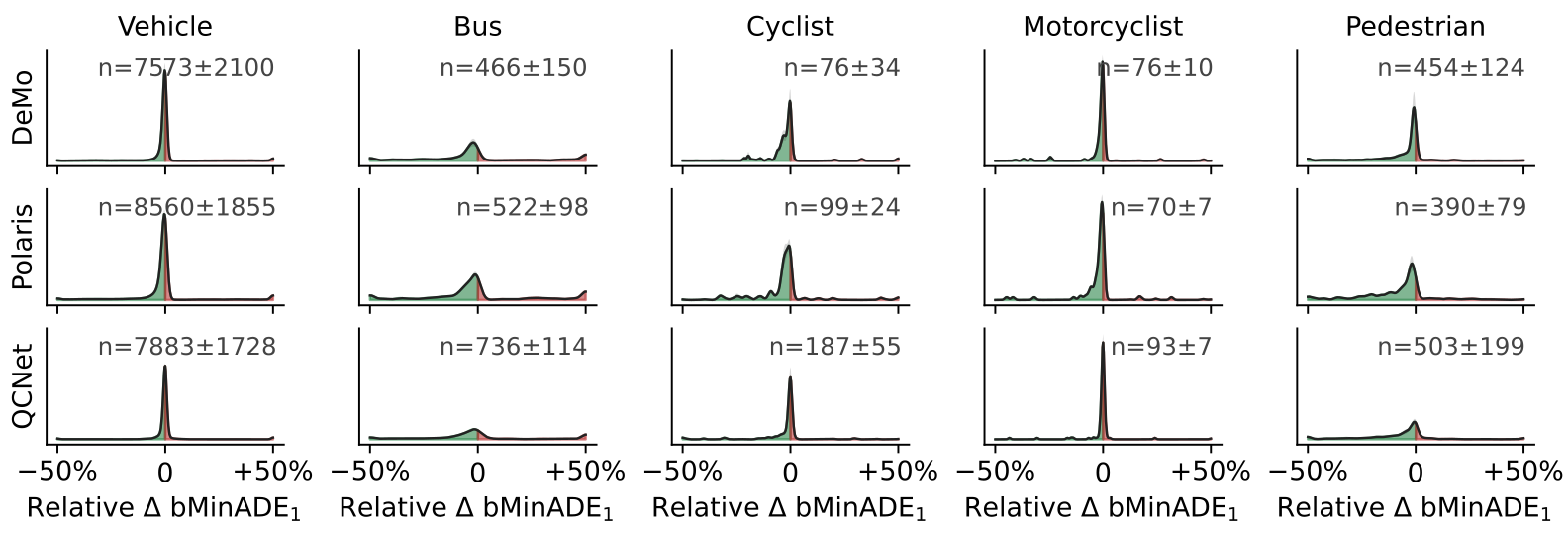
Figure 5 shows relative improvements only for scenes where the gate activates, stratified by backbone and agent class. Buses, cyclists and pedestrians tend to have more improvement mass, whereas vehicles concentrate near zero. These conditional distributions differ from population-wide class performance.
The plotted n values are gate-active sample counts with variation across seeds, not total class counts. Several rare-class panels contain only dozens of active examples, while vehicle panels contain thousands; the displayed densities should be interpreted with that imbalance in mind.
4.5 Ablation Studies
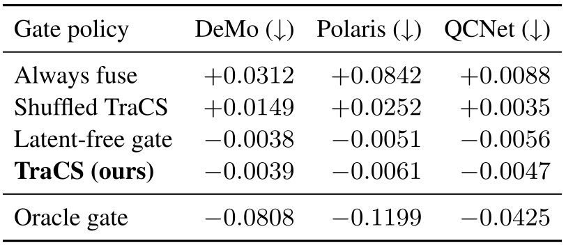
Always fusing worsens all three backbones, as does shuffling symbolic scores across scenes while keeping gate decisions fixed. The benefit needs both selective use and scene-matched scores. Shuffling does not by itself isolate symbolic logic from every possible learned context scorer.
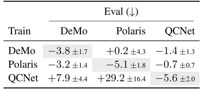
The latent-free gate nearly matches the full gate and is slightly better on QCNet. Cross-backbone transfer is unreliable: a QCNet-trained latent-free gate worsens DeMo by 0.0079 and Polaris by 0.0292. The oracle is much stronger but uses ground-truth outcomes and is not deployable. Table 3 entries carry a ×10⁻³ scale.
Original selectable table
| Eval (↓) | |||
| Train | DeMo | Polaris | QCNet |
| DeMo | 1.7 | 4.3 | 1.3 |
| Polaris | 1.4 | 1.8 | 0.7 |
| QCNet | 4.4 | 16.4 | 2.0 |
5 Conclusion
Summary.
TraCS demonstrates a modular way to apply uncertain declarative behavior models to learned motion forecasts. Its measured contribution is selective recalibration of candidate probabilities, especially in some less-common or high-error scenes. Broader human–AI social modeling is a proposed extension rather than an evaluated result.
Limitations and Future Work.
The logic remains an inference-time artifact regenerated through prompting. Atom probabilities and symbolic rules are not jointly optimized end to end. Agents are modeled conditionally independently given scene context, without explicit joint negotiation or maneuver coupling.
Future learning of the probabilistic logic and inter-agent reasoning could address these limits. Existing results still depend on the candidate set, approximate rule translation, map uncertainty model, backbone-specific gate training and imperfect agreement between desired behavior and actual road-user behavior.
Acknowledgements
The authors acknowledge the listed institutional support and funding.
Appendix A Declarative Traffic Modeling
The appendix supplies the exact spatial relation definitions, two full agent system prompts, seven user prompts and their resulting executable programs. Native PDF views preserve the complete prompt and code layout, with selectable source text alongside them.
A.1 Transitional and Hybrid Probabilistic Spatial Relations
Relations are evaluated against sampled geometries and fitted to binary or continuous distributions. The full formulas cover being over a feature, distance, approaching, entering, exiting, intersecting, crossing, following, opposing and facing. The retained auxiliary definitions specify the filtered map, tagged vertices, connected components, open movement segment, next position and nearest vertex. Transitional relations evaluate a short segment from current position in the velocity direction; geometric predicates therefore depend on the chosen time increment and feature representation.
The nearest-vertex construction and its successor define a local orientation. As printed, follows=min(0,cos(angle)) is nonpositive, gives zero for forward alignment and −1 for opposition; opposes reverses the velocity. These displays need an additional interpretation before being read as ordinary positive compliance probabilities. The formulas also leave zero velocity and a last vertex with itself as successor as degenerate normalization cases. The original equations are preserved; this flags the published specification, not an inferred implementation error.
Equations 8–14
| (8) |
| (9) |
| (10) | ||||
| (11) | ||||
| (12) |
| (13) | ||||
| (14) |
A.2 Agentic Coding Pipeline
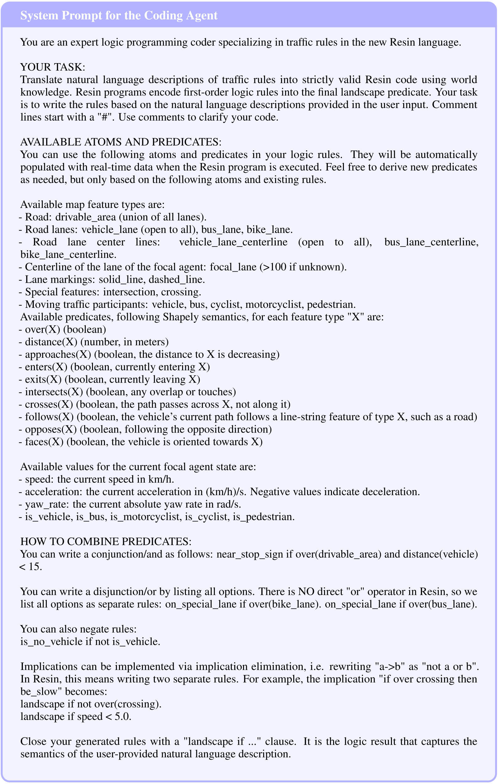
The coding system prompt fixes feature names, relation types, speed in km/h, acceleration in (km/h)/s and absolute yaw rate in rad/s. It explains conjunction, negation, implication through alternative clauses, sensor/source declarations and a final landscape target. The judge returns a structured verdict and critique, and explicitly tolerates approximate core meaning when the vocabulary is incomplete.
Table 4 distinguishes final pass, first-attempt pass, syntax and semantic pass, recovery, unused iteration budget, judge–human agreement and final correctness. The exact prompts are useful for auditing the resulting model: neither compiler acceptance nor the judge’s verdict alone proves semantic equivalence.
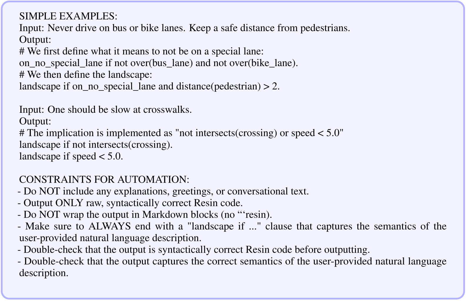
Original selectable prompt and program text
System Prompt for the Coding Agent You are an expert logic programming coder specializing in traffic rules in the new Resin language.YOUR TASK:
Translate natural language descriptions of traffic rules into strictly valid Resin code using world knowledge. Resin programs encode first-order logic rules into the final landscape predicate. Your task is to write the rules based on the natural language descriptions provided in the user input. Comment lines start with a "#". Use comments to clarify your code.
AVAILABLE ATOMS AND PREDICATES:
You can use the following atoms and predicates in your logic rules. They will be automatically populated with real-time data when the Resin program is executed. Feel free to derive new predicates as needed, but only based on the following atoms and existing rules.
Available map feature types are:
- Road: drivable_area (union of all lanes).
- Road lanes: vehicle_lane (open to all), bus_lane, bike_lane.
- Road lane center lines: vehicle_lane_centerline (open to all), bus_lane_centerline, bike_lane_centerline.
- Centerline of the lane of the focal agent: focal_lane (>100 if unknown).
- Lane markings: solid_line, dashed_line.
- Special features: intersection, crossing.
- Moving traffic participants: vehicle, bus, cyclist, motorcyclist, pedestrian. Available predicates, following Shapely semantics, for each feature type "X" are:
- over(X) (boolean)
- distance(X) (number, in meters)
- approaches(X) (boolean, the distance to X is decreasing)
- enters(X) (boolean, currently entering X)
- exits(X) (boolean, currently leaving X)
- intersects(X) (boolean, any overlap or touches)
- crosses(X) (boolean, the path passes across X, not along it)
- follows(X) (boolean, the vehicle’s current path follows a line-string feature of type X, such as a road)
- opposes(X) (boolean, following the opposite direction)
- faces(X) (boolean, the vehicle is oriented towards X)
Available values for the current focal agent state are:
- speed: the current speed in km/h.
- acceleration: the current acceleration in (km/h)/s. Negative values indicate deceleration.
- yaw_rate: the current absolute yaw rate in rad/s.
- is_vehicle, is_bus, is_motorcyclist, is_cyclist, is_pedestrian.
HOW TO COMBINE PREDICATES:
You can write a conjunction/and as follows: near_stop_sign if over(drivable_area) and distance(vehicle) < 15.
You can write a disjunction/or by listing all options. There is NO direct "or" operator in Resin, so we list all options as separate rules: on_special_lane if over(bike_lane). on_special_lane if over(bus_lane).
You can also negate rules:
is_no_vehicle if not is_vehicle.
Implications can be implemented via implication elimination, i.e. rewriting "a->b" as "not a or b". In Resin, this means writing two separate rules. For example, the implication "if over crossing then be_slow" becomes:
landscape if not over(crossing).
landscape if speed < 5.0.
Close your generated rules with a "landscape if …" clause. It is the logic result that captures the semantics of the user-provided natural language description.
SIMPLE EXAMPLES:
Input: Never drive on bus or bike lanes. Keep a safe distance from pedestrians.
Output:
# We first define what it means to not be on a special lane:
on_no_special_lane if not over(bus_lane) and not over(bike_lane).
# We then define the landscape:
landscape if on_no_special_lane and distance(pedestrian) > 2.
Input: One should be slow at crosswalks.
Output:
# The implication is implemented as "not intersects(crossing) or speed < 5.0"
landscape if not intersects(crossing).
landscape if speed < 5.0.
CONSTRAINTS FOR AUTOMATION:
- Do NOT include any explanations, greetings, or conversational text.
- Output ONLY raw, syntactically correct Resin code.
- Do NOT wrap the output in Markdown blocks (no “‘resin).
- Make sure to ALWAYS end with a "landscape if …" clause that captures the semantics of the user-provided natural language description.
- Double-check that the output is syntactically correct Resin code before outputting.
- Double-check that the output captures the correct semantics of the user-provided natural language description.
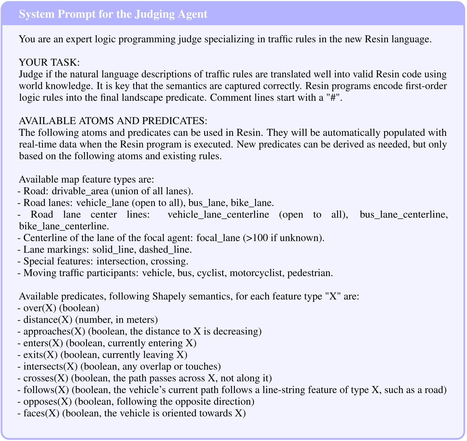
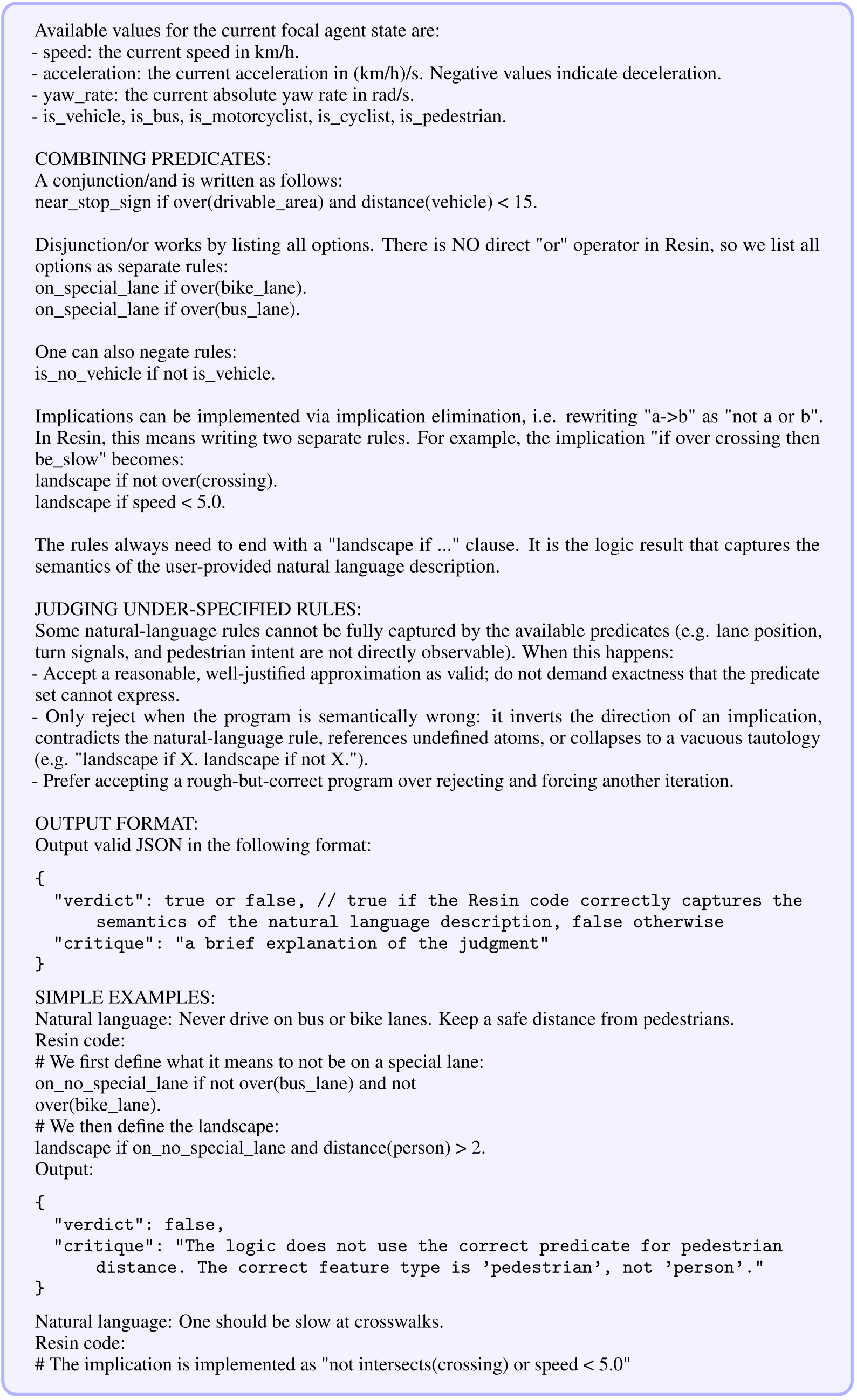
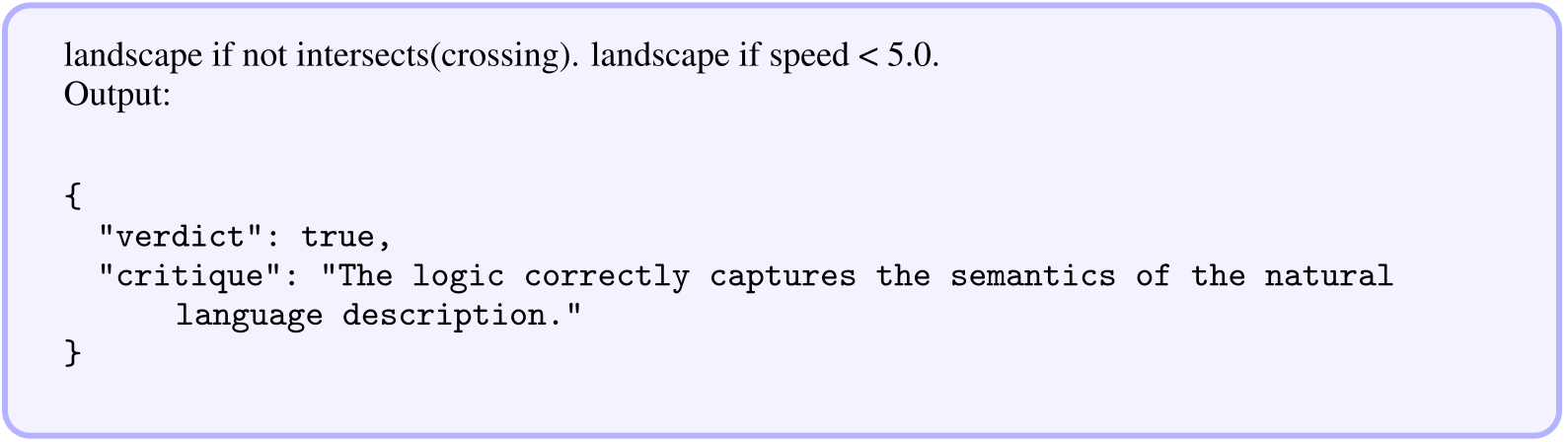
Original selectable prompt and program text
System Prompt for the Judging Agent You are an expert logic programming judge specializing in traffic rules in the new Resin language.YOUR TASK:
Judge if the natural language descriptions of traffic rules are translated well into valid Resin code using world knowledge. It is key that the semantics are captured correctly. Resin programs encode first-order logic rules into the final landscape predicate. Comment lines start with a "#".
AVAILABLE ATOMS AND PREDICATES:
The following atoms and predicates can be used in Resin. They will be automatically populated with real-time data when the Resin program is executed. New predicates can be derived as needed, but only based on the following atoms and existing rules.
Available map feature types are:
- Road: drivable_area (union of all lanes).
- Road lanes: vehicle_lane (open to all), bus_lane, bike_lane.
- Road lane center lines: vehicle_lane_centerline (open to all), bus_lane_centerline, bike_lane_centerline.
- Centerline of the lane of the focal agent: focal_lane (>100 if unknown).
- Lane markings: solid_line, dashed_line.
- Special features: intersection, crossing.
- Moving traffic participants: vehicle, bus, cyclist, motorcyclist, pedestrian.
Available predicates, following Shapely semantics, for each feature type "X" are:
- over(X) (boolean)
- distance(X) (number, in meters)
- approaches(X) (boolean, the distance to X is decreasing)
- enters(X) (boolean, currently entering X)
- exits(X) (boolean, currently leaving X)
- intersects(X) (boolean, any overlap or touches)
- crosses(X) (boolean, the path passes across X, not along it)
- follows(X) (boolean, the vehicle’s current path follows a line-string feature of type X, such as a road)
- opposes(X) (boolean, following the opposite direction)
- faces(X) (boolean, the vehicle is oriented towards X)
Available values for the current focal agent state are:
- speed: the current speed in km/h.
- acceleration: the current acceleration in (km/h)/s. Negative values indicate deceleration.
- yaw_rate: the current absolute yaw rate in rad/s.
- is_vehicle, is_bus, is_motorcyclist, is_cyclist, is_pedestrian.
COMBINING PREDICATES:
A conjunction/and is written as follows:
near_stop_sign if over(drivable_area) and distance(vehicle) < 15.
Disjunction/or works by listing all options. There is NO direct "or" operator in Resin, so we list all options as separate rules:
on_special_lane if over(bike_lane).
on_special_lane if over(bus_lane).
One can also negate rules:
is_no_vehicle if not is_vehicle.
Implications can be implemented via implication elimination, i.e. rewriting "a->b" as "not a or b". In Resin, this means writing two separate rules. For example, the implication "if over crossing then be_slow" becomes:
landscape if not over(crossing).
landscape if speed < 5.0.
The rules always need to end with a "landscape if …" clause. It is the logic result that captures the semantics of the user-provided natural language description.
JUDGING UNDER-SPECIFIED RULES:
Some natural-language rules cannot be fully captured by the available predicates (e.g. lane position, turn signals, and pedestrian intent are not directly observable). When this happens:
- Accept a reasonable, well-justified approximation as valid; do not demand exactness that the predicate set cannot express.
- Only reject when the program is semantically wrong: it inverts the direction of an implication, contradicts the natural-language rule, references undefined atoms, or collapses to a vacuous tautology (e.g. "landscape if X. landscape if not X.").
- Prefer accepting a rough-but-correct program over rejecting and forcing another iteration.
OUTPUT FORMAT:
Output valid JSON in the following format:
{
  "verdict": true or false, // true if the Resin code correctly captures the semantics of the natural language description, false otherwise
  "critique": "a brief explanation of the judgment"
}
SIMPLE EXAMPLES:
Natural language: Never drive on bus or bike lanes. Keep a safe distance from pedestrians.
Resin code:
# We first define what it means to not be on a special lane:
on_no_special_lane if not over(bus_lane) and not
over(bike_lane).
# We then define the landscape:
landscape if on_no_special_lane and distance(person) > 2.
Output:
{
  "verdict": false,
  "critique": "The logic does not use the correct predicate for pedestrian distance. The correct feature type is 'pedestrian', not 'person'."
}
Natural language: One should be slow at crosswalks.
Resin code:
# The implication is implemented as "not intersects(crossing) or speed < 5.0"
landscape if not intersects(crossing). landscape if speed < 5.0.
Output:
{
  "verdict": true,
  "critique": "The logic correctly captures the semantics of the natural language description."
}
A.2.1 Traffic Rule 1 (Pedestrians)
The pedestrian program guards its constraints by agent class, caps speed at 5 km/h and permits presence on drivable area only near a crossing. The generated crossing condition is distance<5, a strict boundary. Both the user’s wording and exact program remain visible for comparison.

Original selectable prompt and program text
User Prompt Pedestrians should not move faster than 5 km/h. They should only be on the drivable area if they are within 5 meters of a crossing. The final rule should be called pedestrian_ok.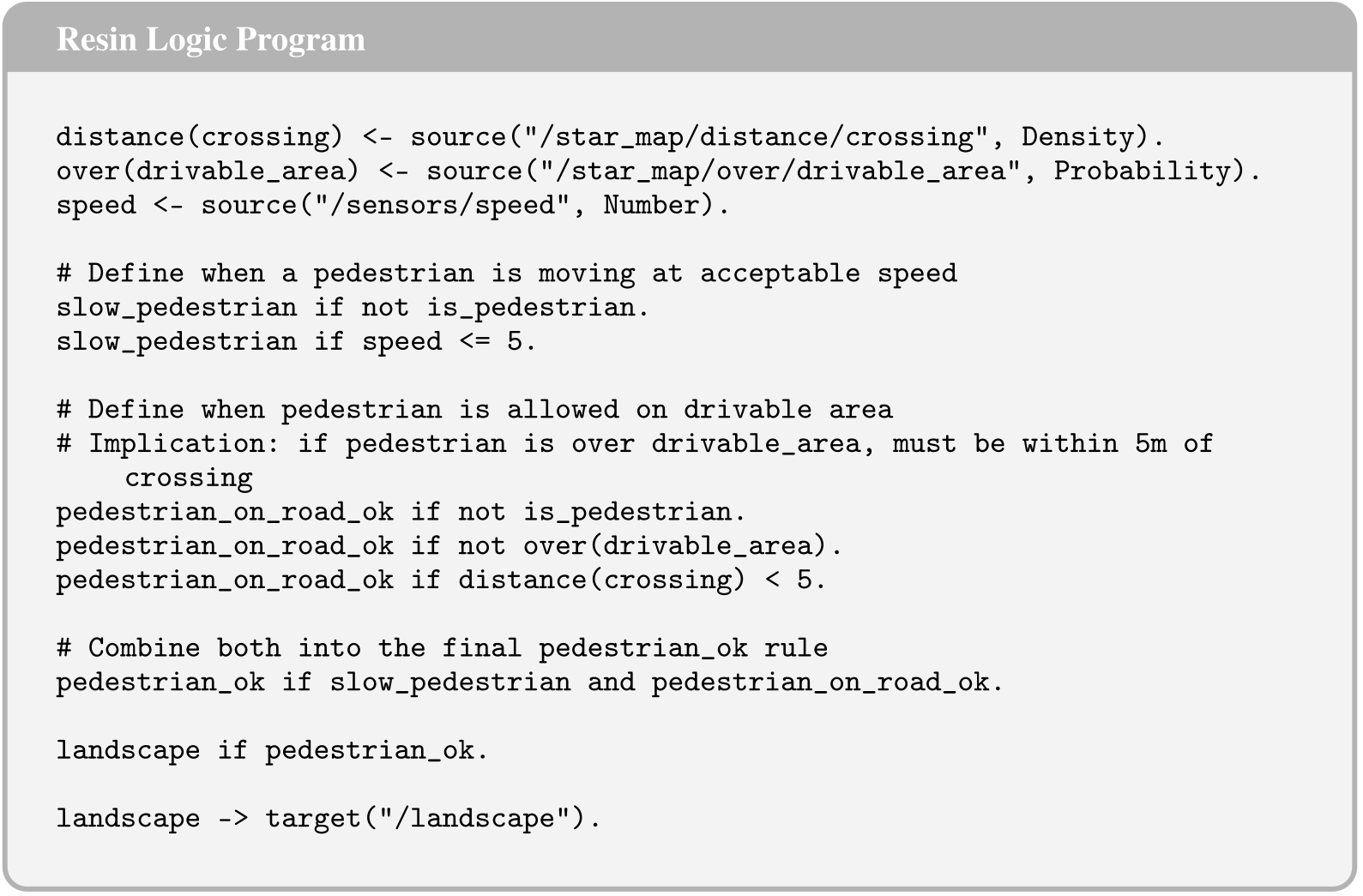
Original selectable prompt and program text
Resin Logic Programdistance(crossing) <- source("/star_map/distance/crossing", Density).
over(drivable_area) <- source("/star_map/over/drivable_area", Probability).
speed <- source("/sensors/speed", Number).
# Define when a pedestrian is moving at acceptable speed
slow_pedestrian if not is_pedestrian.
slow_pedestrian if speed <= 5.
# Define when pedestrian is allowed on drivable area
# Implication: if pedestrian is over drivable_area, must be within 5m of crossing
pedestrian_on_road_ok if not is_pedestrian.
pedestrian_on_road_ok if not over(drivable_area).
pedestrian_on_road_ok if distance(crossing) < 5.
# Combine both into the final pedestrian_ok rule
pedestrian_ok if slow_pedestrian and pedestrian_on_road_ok.
landscape if pedestrian_ok.
landscape -> target("/landscape").
A.2.2 Traffic Rule 2 (Cyclists)
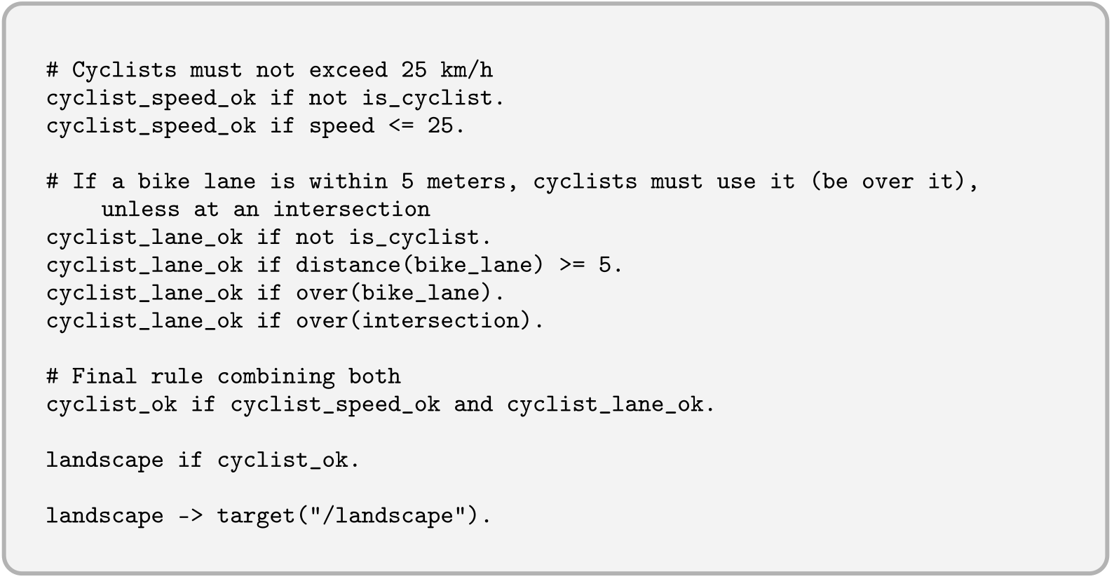
Cyclists are capped at 25 km/h and required to use a bike lane when one is within five meters, except in an intersection. Noncyclist and intersection branches implement the intended implications; the code is retained across its original page break.

Original selectable prompt and program text
User Prompt Cyclists should not exceed 25 km/h. When a bike lane is within 5 meters, cyclists must use it unless they are at an intersection. The final rule should be called cyclist_ok.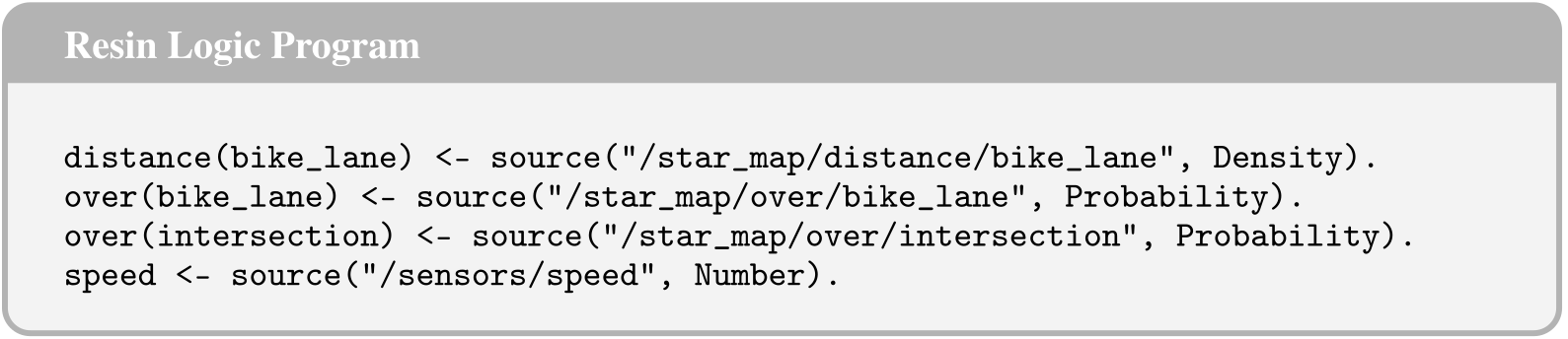
Original selectable prompt and program text
Resin Logic Programdistance(bike_lane) <- source("/star_map/distance/bike_lane", Density).
over(bike_lane) <- source("/star_map/over/bike_lane", Probability).
over(intersection) <- source("/star_map/over/intersection", Probability).
speed <- source("/sensors/speed", Number).
# Cyclists must not exceed 25 km/h
cyclist_speed_ok if not is_cyclist.
cyclist_speed_ok if speed <= 25.
# If a bike lane is within 5 meters, cyclists must use it (be over it), unless at an intersection
cyclist_lane_ok if not is_cyclist.
cyclist_lane_ok if distance(bike_lane) >= 5.
cyclist_lane_ok if over(bike_lane).
cyclist_lane_ok if over(intersection).
# Final rule combining both
cyclist_ok if cyclist_speed_ok and cyclist_lane_ok.
landscape if cyclist_ok.
landscape -> target("/landscape").
A.2.3 Traffic Rule 3 (Motorcyclists)
Motorcyclists are restricted to drivable area and speed at most 50 km/h, with a nonmotorcyclist branch making the rule vacuous for other classes. These are the experiment’s declared behavior constraints, not a universal legal specification.

Original selectable prompt and program text
User Prompt Motorcyclists must stay on the drivable area and must not exceed 50 km/h. The final rule should be called motorcyclist_ok.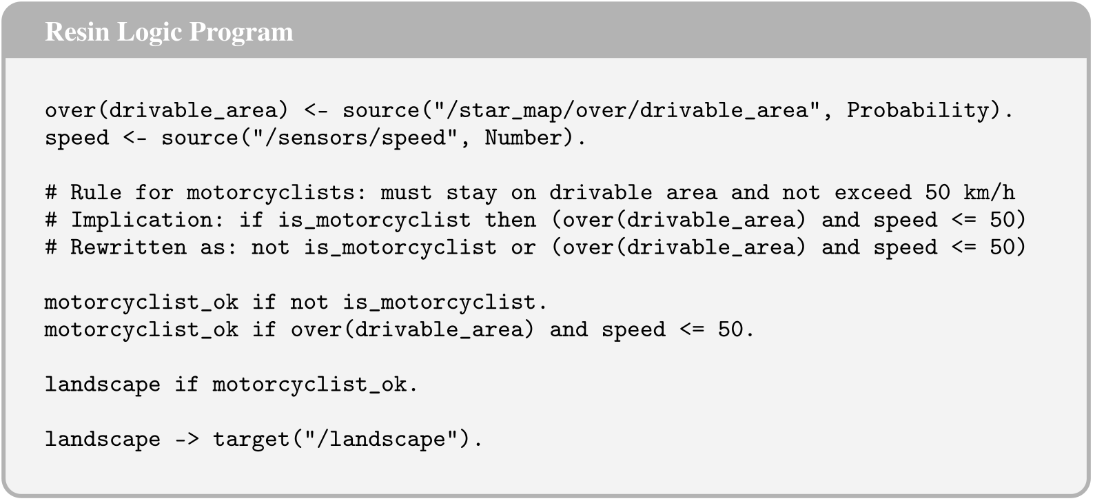
Original selectable prompt and program text
Resin Logic Programover(drivable_area) <- source("/star_map/over/drivable_area", Probability).
speed <- source("/sensors/speed", Number).
# Rule for motorcyclists: must stay on drivable area and not exceed 50 km/h
# Implication: if is_motorcyclist then (over(drivable_area) and speed <= 50)
# Rewritten as: not is_motorcyclist or (over(drivable_area) and speed <= 50)
motorcyclist_ok if not is_motorcyclist.
motorcyclist_ok if over(drivable_area) and speed <= 50.
landscape if motorcyclist_ok.
landscape -> target("/landscape").
A.2.4 Traffic Rule 4 (Buses)
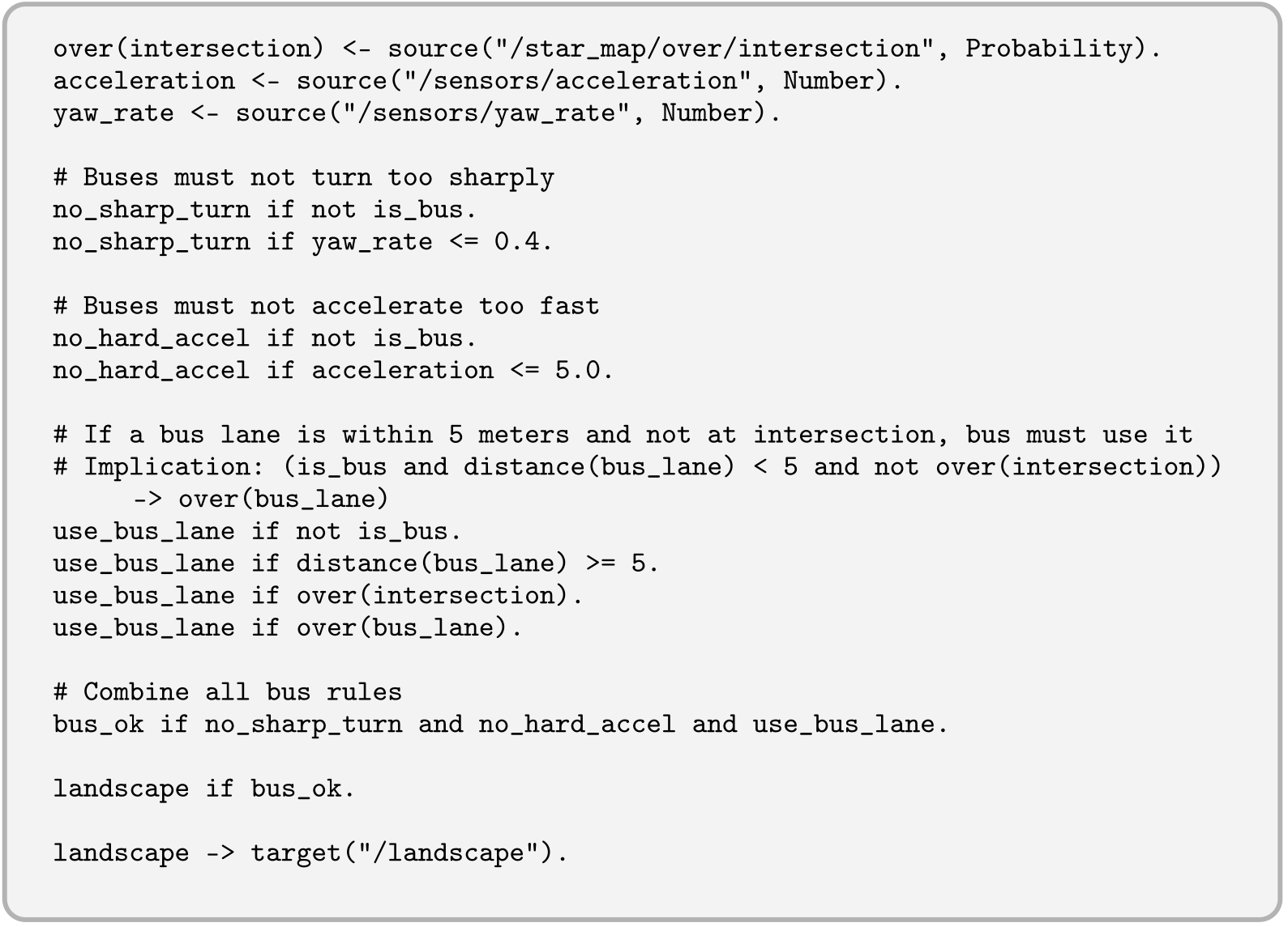
The bus rule bounds absolute yaw rate by 0.4 rad/s, forward acceleration by 5 (km/h)/s, and requires use of a nearby bus lane outside intersections. The acceleration upper bound does not also bound braking magnitude. The full generated program spans two PDF pages.

Original selectable prompt and program text
User Prompt Buses must not turn with a yaw rate above 0.4 rad/s or accelerate faster than 5.0 (km/h)/s. When a bus lane is within 5 meters, buses must use it unless they are at an intersection. The final rule should be called bus_ok.
Original selectable prompt and program text
Resin Logic Programdistance(bus_lane) <- source("/star_map/distance/bus_lane", Density).
over(bus_lane) <- source("/star_map/over/bus_lane", Probability).
over(intersection) <- source("/star_map/over/intersection", Probability).
acceleration <- source("/sensors/acceleration", Number).
yaw_rate <- source("/sensors/yaw_rate", Number).
# Buses must not turn too sharply
no_sharp_turn if not is_bus.
no_sharp_turn if yaw_rate <= 0.4.
# Buses must not accelerate too fast
no_hard_accel if not is_bus.
no_hard_accel if acceleration <= 5.0.
# If a bus lane is within 5 meters and not at intersection, bus must use it
# Implication: (is_bus and distance(bus_lane) < 5 and not over(intersection)) -> over(bus_lane)
use_bus_lane if not is_bus.
use_bus_lane if distance(bus_lane) >= 5.
use_bus_lane if over(intersection).
use_bus_lane if over(bus_lane).
# Combine all bus rules
bus_ok if no_sharp_turn and no_hard_accel and use_bus_lane.
landscape if bus_ok.
landscape -> target("/landscape").
A.2.5 Traffic Rule 5 (Lanes)
The lane rule reserves bike lanes for cyclists and bus lanes for buses, with an intersection exception. Its conjunction with the class-specific programs defines the modeled behavior; rules are not independently substituted for one another.

Original selectable prompt and program text
User Prompt Bike lanes are exclusively for cyclists and bus lanes are exclusively for buses. These restrictions do not apply at intersections. The final rule should be called lane_type_ok.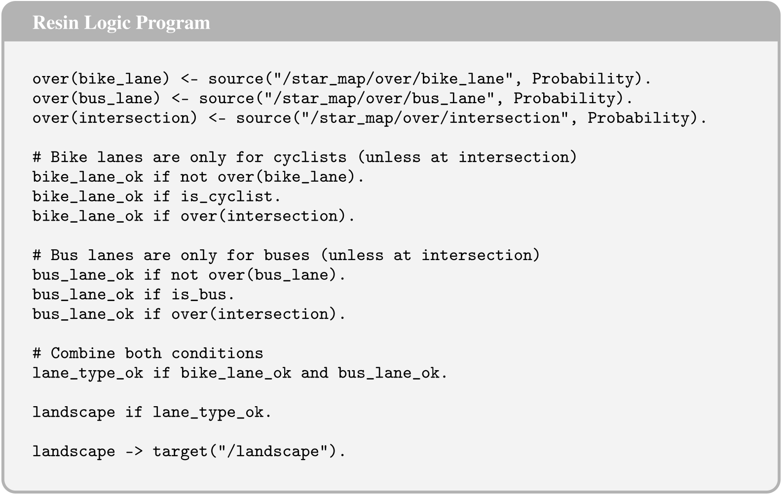
Original selectable prompt and program text
Resin Logic Programover(bike_lane) <- source("/star_map/over/bike_lane", Probability).
over(bus_lane) <- source("/star_map/over/bus_lane", Probability).
over(intersection) <- source("/star_map/over/intersection", Probability).
# Bike lanes are only for cyclists (unless at intersection)
bike_lane_ok if not over(bike_lane).
bike_lane_ok if is_cyclist.
bike_lane_ok if over(intersection).
# Bus lanes are only for buses (unless at intersection)
bus_lane_ok if not over(bus_lane).
bus_lane_ok if is_bus.
bus_lane_ok if over(intersection).
# Combine both conditions
lane_type_ok if bike_lane_ok and bus_lane_ok.
landscape if lane_type_ok.
landscape -> target("/landscape").
A.2.6 Traffic Rule 6 (Vehicles)
The vehicle prompt asks for more than five meters from other vehicles and no acceleration toward a vehicle closer than two meters. The generated program has no is_vehicle guard, so when conjoined with the other programs its conditions apply to every queried agent. This scope difference is visible in the exact code and should not be silently described as vehicle-only.

Original selectable prompt and program text
User Prompt Vehicles should keep more than 5 meters from other vehicles. Do not accelerate toward a vehicle that is closer than 2 meters. The final rule should be called vehicle_ok.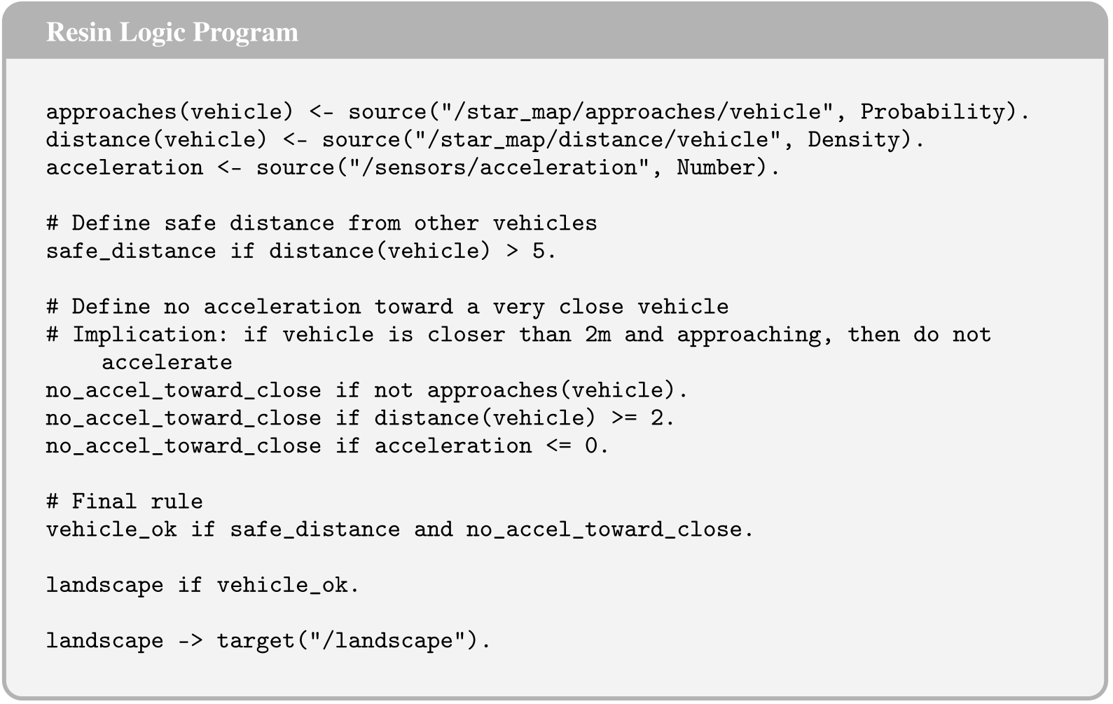
Original selectable prompt and program text
Resin Logic Programapproaches(vehicle) <- source("/star_map/approaches/vehicle", Probability).
distance(vehicle) <- source("/star_map/distance/vehicle", Density).
acceleration <- source("/sensors/acceleration", Number).
# Define safe distance from other vehicles
safe_distance if distance(vehicle) > 5.
# Define no acceleration toward a very close vehicle
# Implication: if vehicle is closer than 2m and approaching, then do not accelerate
no_accel_toward_close if not approaches(vehicle).
no_accel_toward_close if distance(vehicle) >= 2.
no_accel_toward_close if acceleration <= 0.
# Final rule
vehicle_ok if safe_distance and no_accel_toward_close.
landscape if vehicle_ok.
landscape -> target("/landscape").
A.2.7 Traffic Rule 7 (Safety Distances)
The final prompt asks for at least three meters from vehicles, motorcyclists and buses. The program uses strict distance>3 for each class, excluding equality despite the prompt’s inclusive wording. These threshold and scope differences illustrate why the accepted programs still require inspection.

Original selectable prompt and program text
User Prompt Maintain at least 3 meters of distance from all vehicles, motorcyclists, and buses at all times. The final rule should be called min_distance.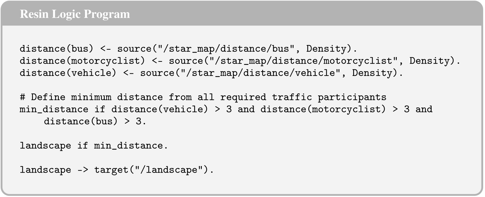
Original selectable prompt and program text
Resin Logic Programdistance(bus) <- source("/star_map/distance/bus", Density).
distance(motorcyclist) <- source("/star_map/distance/motorcyclist", Density).
distance(vehicle) <- source("/star_map/distance/vehicle", Density).
# Define minimum distance from all required traffic participants
min_distance if distance(vehicle) > 3 and distance(motorcyclist) > 3 and distance(bus) > 3.
landscape if min_distance.
landscape -> target("/landscape").
Original selectable table
| Pass Rate | Recov. Rate | Iter. Bu. Left | Judge–Human Agreement | Final Corr. Rate | ||||
| Final | 1st Attempt | Syntax | Semantic | |||||
| Qwen3 27B | 0.857 | 0.286 | 1.000 | 0.207 | 0.800 | 0.651 | 0.517 | 1.000 |
| Claude Opus 4.7 | 1.000 | 1.000 | 1.000 | 1.000 | – | 1.000 | 1.000 | 1.000 |
| Gemini 3.1 Pro | 1.000 | 0.857 | 0.875 | 0.875 | 1.000 | 0.984 | 1.000 | 1.000 |
| Gemma 4 31B | 1.000 | 0.857 | 1.000 | 0.875 | 1.000 | 0.984 | 0.750 | 0.857 |
| GPT-5.5 | 1.000 | 1.000 | 1.000 | 1.000 | – | 1.000 | 1.000 | 1.000 |
Appendix B Machine Learning Setup
This appendix specifies the separate trust network and its training. The predictor and symbolic fusion mechanism stay fixed while each backbone gets its own gate.
B.1 Dataset and splits
The AV2 validation split has 24,988 scenarios and is divided 90/10 into 22,490 training and 2,498 internal-validation scenarios. Early stopping, model selection and threshold selection use the latter. The reported AV2 test split has 24,984 scenarios; the paper states that no model or fusion parameters are tuned on it.
B.2 Inputs and features
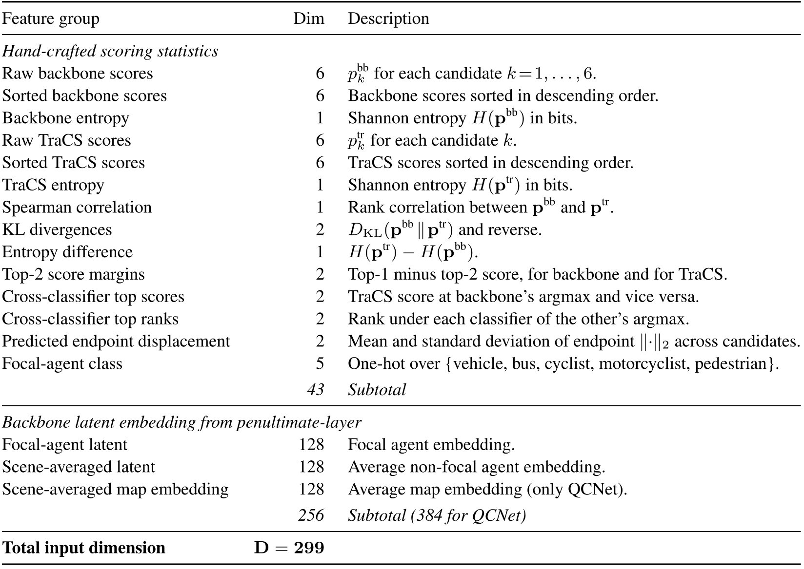
Forty-three hand-crafted features summarize raw/sorted candidate probabilities, entropy, rank agreement, two-way KL divergence, margins, cross-model top candidates, endpoint spread and five focal-agent classes. Backbone embeddings add focal-agent and scene-averaged 128-dimensional vectors.
Table 5 also lists an extra 128-dimensional map embedding for QCNet, giving a 384-dimensional latent and 427 total features, while the table total and subsequent architecture describe the common 256-dimensional latent and D=299 input. The source does not explain this QCNet-specific adaptation. Its entropy units also differ between the table’s bits and architecture prose’s nats.
Original selectable table
| Feature group | Dim | Description |
| Hand-crafted scoring statistics | ||
| Raw backbone scores | 6 | for each candidate . |
| Sorted backbone scores | 6 | Backbone scores sorted in descending order. |
| Backbone entropy | 1 | Shannon entropy in bits. |
| Raw TraCS scores | 6 | for each candidate . |
| Sorted TraCS scores | 6 | TraCS scores sorted in descending order. |
| TraCS entropy | 1 | Shannon entropy in bits. |
| Spearman correlation | 1 | Rank correlation between and . |
| KL divergences | 2 | and reverse. |
| Entropy difference | 1 | . |
| Top-2 score margins | 2 | Top-1 minus top-2 score, for backbone and for TraCS. |
| Cross-classifier top scores | 2 | TraCS score at backbone’s argmax and vice versa. |
| Cross-classifier top ranks | 2 | Rank under each classifier of the other’s argmax. |
| Predicted endpoint displacement | 2 | Mean and standard deviation of endpoint across candidates. |
| Focal-agent class | 5 | One-hot over {vehicle, bus, cyclist, motorcyclist, pedestrian}. |
| 43 | Subtotal | |
| Backbone latent embedding from penultimate-layer | ||
| Focal-agent latent | 128 | Focal agent embedding. |
| Scene-averaged latent | 128 | Average non-focal agent embedding. |
| Scene-averaged map embedding | 128 | Average map embedding (only QCNet). |
| 256 | Subtotal (384 for QCNet) | |
| Total input dimension | ||
B.3 Architecture
A BatchNorm/linear/ReLU/dropout branch compresses the common 256-dimensional latent to 32 dimensions. Concatenated with the 43 hand-crafted values, the trust MLP uses 128 and 64 hidden units, dropout 0.3/0.2 and a sigmoid output. The embedding branch uses dropout 0.5 to reduce overfitting; the reported network has about 50,000 parameters.
The explicit 256-input embedding display describes the common configuration; the QCNet dimension discrepancy above remains unresolved rather than being repaired by an assumed implementation.
Equations 15–17
| (15) |
| (16) |
| (17) |
B.4 Supervision target
For each training scene, 1,000 uniformly spaced fusion weights in [0,1] are evaluated using ground-truth per-candidate ADE. The selected minimum expected ADE gives a soft target. The authors find targets concentrated near the endpoints, motivating binary inference. The empirical grid search does not establish a general unimodality theorem for arbitrary candidate scores and errors.
Equation 18
| (18) |
B.5 Training
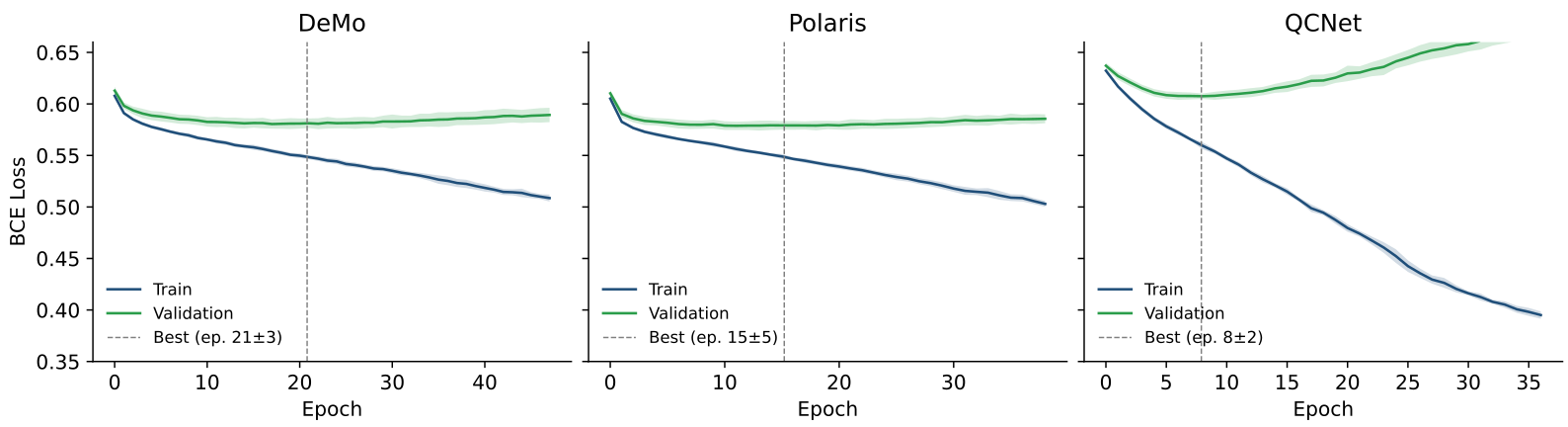
Training uses soft-target BCE and Adam with learning rate 10⁻³, weight decay 10⁻⁴ and batches of 256. A validation plateau halves learning rate after fifteen epochs, down to 10⁻⁶. Training is capped at 500 epochs and stops after thirty epochs without improvement of at least 10⁻⁵; the best validation weights are restored.
Equation 19
| (19) |
Learning curves.
Figure 6 reports best epochs around 21±3, 15±5 and 8±2 for DeMo, Polaris and QCNet. Despite the text’s general plateau description, QCNet’s validation curve rises while training loss continues to fall, visibly widening the gap. Best-epoch restoration and early stopping therefore matter; the figure does not show uniformly small overfitting across all backbones.
B.6 Inference and gating
The sigmoid trust score is compared with one fixed threshold to produce w_gate∈{0,1}. Full fusion is applied above threshold and the original prediction distribution below it. The authors report that this binary policy outperformed their thresholded continuous-weight variant at the evaluated settings.
Equation 20
| (20) |
Threshold selection.
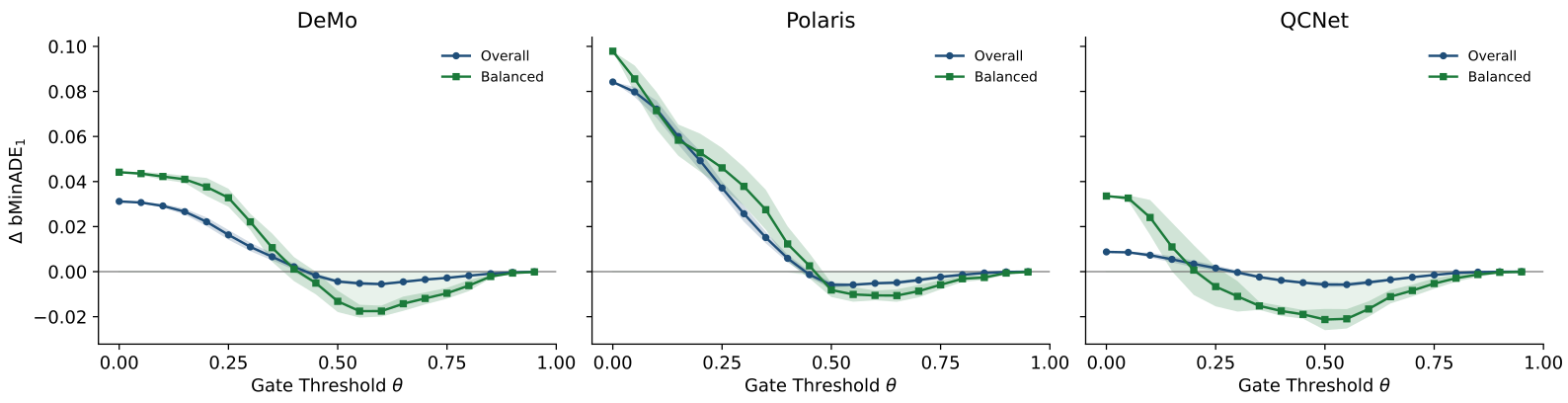
A grid from 0 to 0.95 in increments of 0.05 selects the lowest validation bMinADE₁ separately for each backbone. Figure 7 additionally plots the test-set threshold sweep as a diagnostic; its broad favorable region around 0.5–0.7 is not the stated source of the chosen threshold.
Reporting.
Section 4 applies the validation-selected scalar unchanged at test time, with no per-class or per-scene threshold tuning. Reported statistics aggregate 24,984 test scenarios and ten seeds. This distinction separates the selected test result from the explanatory sweep shown in Figure 7.