Reading guide
All twenty-one pages, nine complete figures, three tables, seventeen numbered equation groups, two proof displays, both theorem statements, the full proof and sixty-one references are covered. CORD-SLS combines a contact-aware simulator with robust output-feedback planning; analytical policy gradients are a separate learning experiment. Its safety statements require valid finite-horizon tubes, calibrated disturbances and bounded state-estimation error. The hardware's fixed 3 cm radius with 87% calibration coverage does not itself establish a specified trajectory-level confidence guarantee.
At a glance
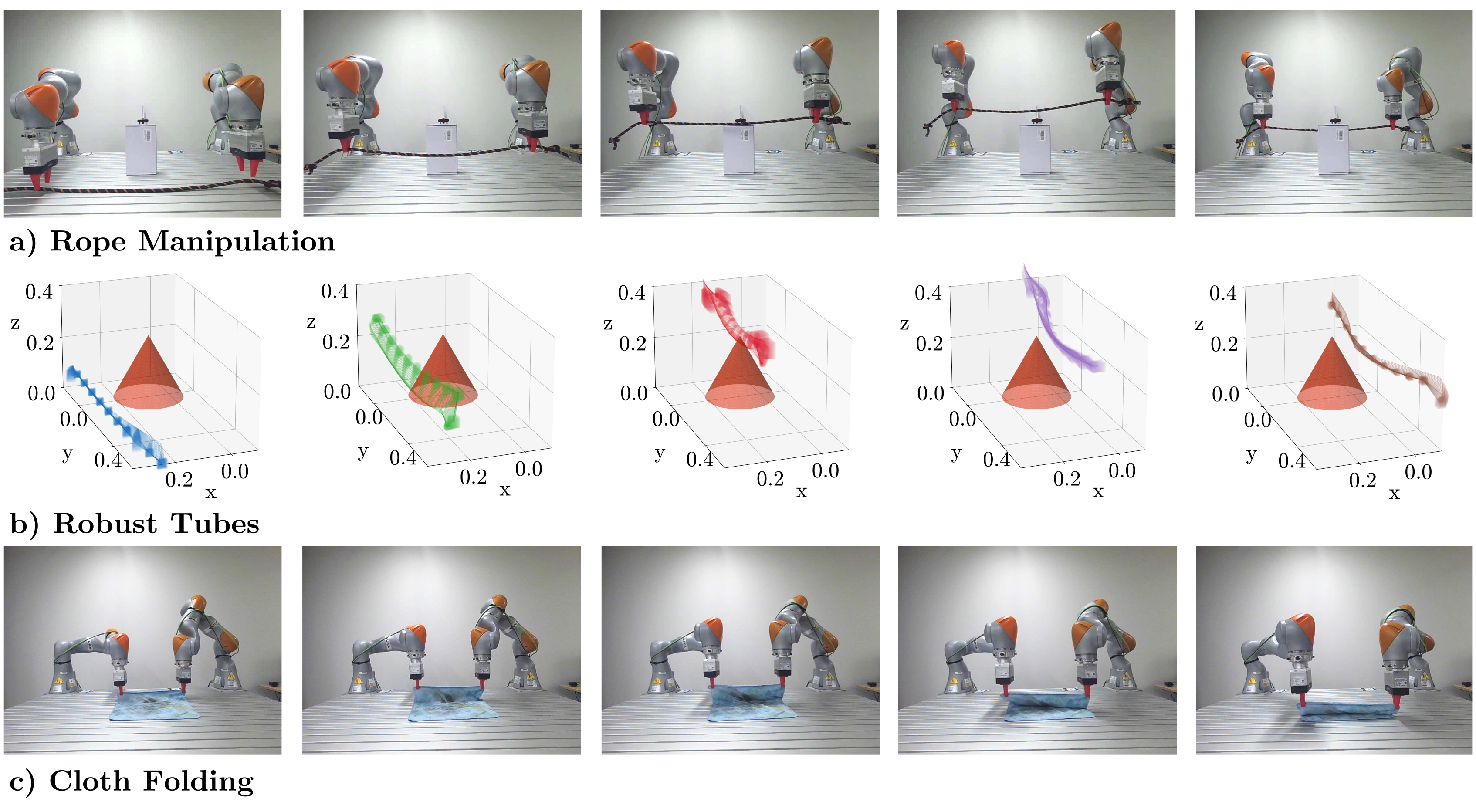
A GPU-parallel simulator supplies contact-seeking surrogate gradients while preserving nonsmooth forward rollouts. Parallel system-level synthesis propagates model and measurement uncertainty to tighten constraints. The experiments compare rope and cloth planning, policy learning and a small hardware demonstration. Main-table planning takes 50–70 ms for rope and 711–758 ms for cloth, while policy inference is faster. The useful result is efficient contact-aware planning with explicitly conditional robustness, rather than an unconditional safety certificate for every deployed perception and replanning pipeline.
1 Introduction
Rope and cloth have many coordinates, intermittent contact and uncertain state estimates. Nominal plans may fail when these uncertainties are ignored, while sparse-contact RL is difficult to explore. The framework combines differentiable contact discovery, output-feedback reachable tubes and aggregate residual calibration. Each part addresses a different problem: the simulator supports optimization, SLS bounds specified disturbances, and conformal prediction supplies a statistical radius under its stated data assumptions.
2 Related Work
Related work spans deformable simulation, differentiable contact, learned/geometric planners and robust control. CORD-SLS integrates these components rather than replacing physical modeling or state estimation. Runtime comparisons depend on simulator representation, compilation and hardware; a faster quasi-static model does not imply greater fidelity to transient deformation.
Deformable Object Simulation
Position-based methods trade fidelity for tractability, while rod/shell models represent richer bending, twisting and friction. The paper uses a convex contact relaxation and surrogate smoothing to obtain useful optimization directions. DEFORM, DaXBench and smoothing-error reachable tubes are relevant comparisons. The chosen elastic model captures stretch and bending; it does not explicitly retain all twisting degrees of freedom of the rod baseline.
Planning
The method extends GPU-SLS from state to output feedback, drawing on Vision-SLS. Prior abstractions and learned models can plan useful motions but do not automatically bound contact and perception error. The new integration still depends on a known state representation, task costs/constraints and valid uncertainty assumptions. Recursive feasibility under repeated replanning is a separate issue discussed in AppendixD.
3 Problem Statement
Equation 1 models bounded process disturbances and delayed noisy observations, and Equation 2 defines the planner's simulator. The state includes deformable nodes and actuated coordinates. The desired output-feedback controller may use observation history, while safety is expressed over state/control constraints. The original HTML entirely omits Equation 1 a/b; both equations are restored from the PDF with selectable mathematical text. Full-state visual reconstruction in the hardware implementation is an additional modeling choice, not direct ground-truth state access.
Original mathematical definitions, assumptions and evaluation protocol
We consider a known state representation for a deformable object of interest (e.g., 3D positions of links for rope, or of mesh node positions for cloth) actuated by control input and governed by uncertain dynamics (1a), where . To account for perception latency, we model the system as being observed with uncertain time-delayed measurements according to an observation map (1b),

Original selectable mathematical display
Equations 1a–1b
| (1a) | |
| (1b) |
Original mathematical definitions, assumptions and evaluation protocol
where and and and are bounded disturbances. We aim to design 1) a differentiable deformable object simulator that approximates the dynamics (1a) while remaining friendly for planning and learning, and 2) an efficient and robust planning and control algorithm that uses this simulator to solve reachability-aware MPC problems for safe deformable object manipulation. We consider two specific problems:

Original selectable mathematical display
Equation 2
| (2) |
Original mathematical definitions, assumptions and evaluation protocol
Problem 2. Reachability-informed MPC for robust deformable manipulation. Optimize a nominal length- state and control trajectory that is feasible for the simulator dynamics (2), together with a causal output-feedback controller , where stabilizes the true deformable dynamics (1a) about using the history of observations, and ensures closed-loop satisfaction of state and control constraints .
4 Method
The approach has four components: implicit deformable simulation, GPU-parallel output-feedback SLS, analytical policy gradients and conformal residual calibration. Their guarantees and timings should be assessed separately. Smoothing improves optimization directions, but a surrogate gradient is not the exact derivative of the nonsmooth rollout. A calibrated one-step residual radius is not automatically an infinite-horizon or recursively feasible control guarantee.
4.1 Differentiable Deformable Object Simulator with Contact Smoothing
Equations 3–7 define a quasi-static nodal model, stiff holonomic attachments and a two-stage implicit/contact solve. Convex friction-cone constraints approximate contact; they do not make every nonlinear elastic problem globally convex. Equations 8–10 differentiate implicit/KKT systems, reusing forward factorizations. Backward solves and vector–Jacobian products still have computational cost: the claim of no extra cost should be read as avoiding new factorization, not free differentiation. Equations 3/6 print M divided by the squared time step, whereas Equation 7 prints M in its Hessian; the original convention is retained and needs reconciliation when reproducing the implementation. Contact smoothing biases gradients only; forward predictions remain nonsmooth. It helps discover contact without guaranteeing every gradient step solves the physical task.
Original mathematical definitions, assumptions and evaluation protocol
Consider a nodal system with nodes, whose 3D coordinates, together with the actuated degrees of freedom (DoFs), form the configuration vector , where . For an elastic energy , the corresponding internal elastic force is given by . Under a quasi-static assumption, the system satisfies

Original selectable mathematical display
Equation 3
| (3) |
Original mathematical definitions, assumptions and evaluation protocol
where is the mass matrix, are the external generalized forces, including gravity acting on the nodal system and actuation forces applied to the actuated DoFs, is the th constraint force, is the discrete timestep, and is the corresponding constraint Jacobian. Both the elastic and constraint forces are evaluated at the next time step, yielding an implicit time-stepping scheme for improved numerical stability. For holonomic constraints, such as a gripper rigidly interacting with the nodal system, we suppose an active constraint enforces the gripper attachment. The next configuration and constraint force must satisfy the complementarity condition

Original selectable mathematical display
Equation 4
| (4) |
Original mathematical definitions, assumptions and evaluation protocol
where the constraint Jacobian is defined as . For contact constraints, we adopt Anitescu’s convex relaxation [53]. Here, the next step configuration and contact force satisfy

Original selectable mathematical display
Equation 5
| (5) |
Original mathematical definitions, assumptions and evaluation protocol
where is the signed distance of contact pair , is the friction cone, and is its dual cone.
Original mathematical definitions, assumptions and evaluation protocol
Simulation Solver We solve the dynamics in (3) subject to the holonomic and contact constraints in (4) and (5) using a two-stage procedure. The first stage computes the system response under the holonomic constraints, while the second stage resolves contact interactions. In the first stage, we solve for an intermediate configuration satisfying

Original selectable mathematical display
Equation 6
| (6) |
Original mathematical definitions, assumptions and evaluation protocol
where denotes the number of holonomic constraints, and is a diagonal stiffness matrix associated with the th holonomic constraint. When the constraint is active, is chosen sufficiently large to enforce (4); otherwise, . (6) is solved using Newton’s method and implicitly defines a mapping from the current configuration to the intermediate configuration . In the second stage, we solve the optimization problem

Original selectable mathematical display
Equation 7
| (7) | ||||
Original mathematical definitions, assumptions and evaluation protocol
The KKT conditions of (7) recover the contact constraint in (5) together with , which corresponds to a linearization of the dynamics about the intermediate configuration . Given a pair, solving (6)–(7) gives the next configuration . The solvers for (6)–(7) are implemented in JAX, allowing GPU-accelerated matrix factorizations.
Original mathematical definitions, assumptions and evaluation protocol
Differentiating Through Simulation To obtain gradients through the dynamics, we differentiate through the optimization problems in (6) and (7). Rather than differentiating through the unrolled iterative solvers, we employ implicit differentiation. For the first-stage problem (6), let denote the inputs to the dynamics. Differentiating the implicit equation defining yields

Original selectable mathematical display
Equation 8
| (8) |

Original selectable mathematical display
Equation 9
| (9) |
Original mathematical definitions, assumptions and evaluation protocol
where denotes the KKT matrix of the optimization problem. The simulator can thus be treated as a differentiable layer. For a scalar objective , the adjoint with respect to is given by

Original selectable mathematical display
Equation 10
| (10) |
Original mathematical definitions, assumptions and evaluation protocol
This expression naturally defines a custom backward pass for the simulator layer. Starting from the adjoint of , we first solve a linear system involving and compute a vector-Jacobian product with to obtain the adjoint of . We then solve a second linear system involving and compute a vector-Jacobian product with to obtain the adjoint of . Since the factorization of and are byproducts of the forward solve, the backward pass incurs no additional cost.
Original mathematical definitions, assumptions and evaluation protocol
To address this issue, we adopt the idea of surrogate gradients [54], in which the gradient used for planning is replaced by a surrogate estimator that does not correspond to the true gradient obtained by differentiating through the physical rollout. This introduces a controlled bias in exchange for improved gradient information in regimes where the true gradient is uninformative. The holonomic constraint in (4) is active only when , at which point a nonzero stiffness matrix is used in (6) to enforce the constraint. This switching between inactive and active constraints introduces both discontinuities and vanishing gradients. To smooth this transition, we redefine as , where is a smoothing parameter. As , this formulation approaches the original indicator-like activation behavior.
Original mathematical definitions, assumptions and evaluation protocol
The contact constraint in (5), which encodes non-contact, stiction, and sliding regimes, similarly introduces discontinuous and vanishing gradients. We smooth this by relaxing the complementarity condition in (5) to , which recovers the original complementarity constraint when . The smoothed dynamics is used solely for gradient computation and the nonsmooth dynamics are used for forward rollouts, preserving model accuracy.
4.2 Simulator-Informed GPU-Parallel Output Feedback SLS
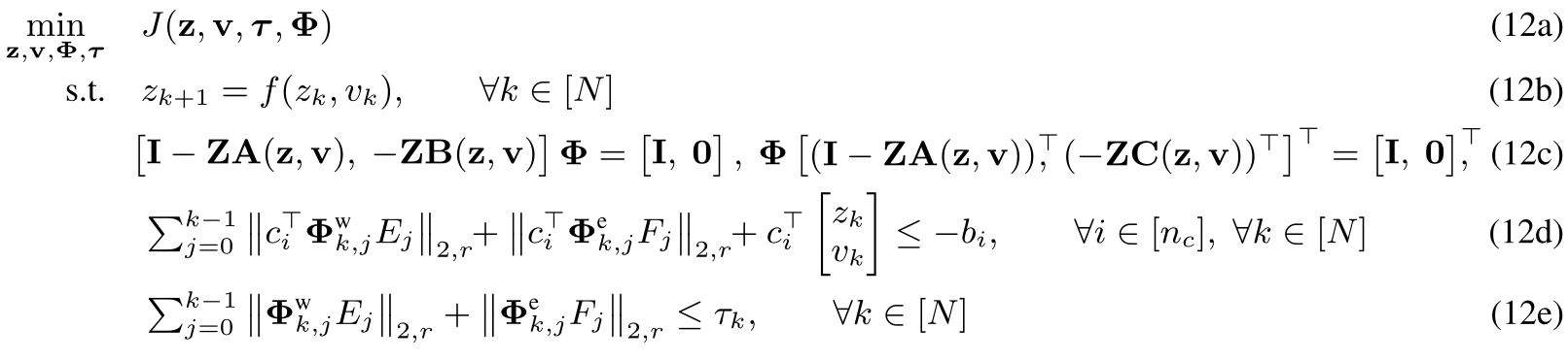
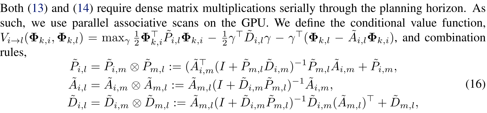
Equations 11–12 formulate finite-horizon robust output feedback and its SLS approximation, using nominal linearizations and row-wise norm bounds to tighten constraints. Equations 13–17 preserve the complete Kalman/observer recursions and associative combination rules, including all five rows of Equation 12. GPU scans reduce serial horizon dependence, while dense state-space operations and memory remain. The text describes affine constraints and refers nonlinear treatment to prior work. Any claimed tube certificate requires valid uncertainty/remainder treatment and successful synthesis; merely plotting a tube or computing a surrogate Jacobian does not establish those prerequisites for arbitrary nonlinear contact dynamics.
Original mathematical definitions, assumptions and evaluation protocol
To plan robust output feedback policies for the deformable object, we wish to approximately solve the idealized optimization (11) to obtain the output-feedback policy ,

Original selectable mathematical display
Equation 11
| (11) | ||||||||
Original mathematical definitions, assumptions and evaluation protocol
where , denotes the set of possible initial conditions, defines the safe set. While we consider nonlinear constraints in Sec. 5, to simplify notation, we describe the method for the case of affine constraints. Nonlinear constraints can be robustly enforced following the approach of [55]. The dynamics and observations are as defined in (1). To efficiently solve (11), we extend GPU-SLS [49], which is limited to state-feedback (i.e., requires perfect state knowledge), to the output-feedback setting by building on [52]. Following [52], the output-feedback SLS synthesis problem can be written as,
Original selectable mathematical display
Equations 12a–12e
| (12a) | ||||
| s.t. | (12b) | |||
| (12c) | ||||
| (12d) | ||||
| (12e) | ||||
Original mathematical definitions, assumptions and evaluation protocol
where and denote the linearizations of the dynamics and observation models about the nominal trajectory , denotes the row-wise two norm, and and are the corresponding linearized state and observation disturbance scalings. The matrix denotes the block downshift operator, with on the first subdiagonal and zeros elsewhere. The closed-loop response operators and characterize the propagation of process and observation disturbances, respectively, via constraint (12c), and defines the reachable tube width. (12d)–(12e) compute output-feedback reachable tubes under disturbances and , and use them to tighten the constraints so the closed-loop reachable set remains inside . To solve (12), [52] decomposes the optimization into three stages: 1) a nominal trajectory generation , 2) state feedback controller optimization , and lastly 3) an output feedback controller optimization . The first two stages are handled directly by GPU-SLS [49]. We therefore focus on the parallel implementation of the third stage by expressing the observer recursions as associative operators, enabling GPU-parallel prefix scans. An optimal solution of the output controller can be found by one backward Kalman recursion,

Original selectable mathematical display
Equation 13
| (13) | ||||
Original mathematical definitions, assumptions and evaluation protocol
where denotes the initial state uncertainty, and independent forward propagations,

Original selectable mathematical display
Equation 14
| (14) |
Original mathematical definitions, assumptions and evaluation protocol
The matrices and can then be assembled by using and

Original selectable mathematical display
Equation 15
| (15) |
Original selectable mathematical display
Equation 16
| (16) | ||||

Original selectable mathematical display
Equation 17
| (17) |
Original mathematical definitions, assumptions and evaluation protocol
We can then recover Kalman gains through a forward parallel associative scan using (16)–(17) to recover , and then from (13). To retrieve , we use a similar procedure and define the conditional observer propagation for each disturbance injection with combination rule and initialization . We obtain the solution to (14) by a forward parallel associative scan, , and , solving the observer-dependent closed-loop response in logarithmic time, analogous to the complexity of GPU-SLS.
4.3 Accelerating Model-Based RL via Analytical Policy Gradients (APG)
The simulator supports expert-data generation and an analytical policy-gradient learning variant, APG. These learned policies are evaluated separately from the reachability-constrained SLS controller and do not inherit its constraint guarantees. The PPO lift baseline is warm-started with ten CORD-SLS demonstrations; without that assistance it fails to discover contact within the stated interaction budget. Training curves address cost/sample efficiency, whereas main-table endpoints use matched total interaction budgets.
4.4 Calibrated Reachability Guarantees via Conformal Prediction (CP)
Calibration measures the aggregate next perceived-state residual, combining dynamics and perception effects. It does not independently identify latent process noise. Under closed-loop/calibration-score exchangeability, the formal method allocates trajectory miscoverage across steps and selects the augmented finite-sample quantile, returning infinity when too few samples support the requested level. The theorem then assumes valid perceived-state/control containment and inflates state tubes by a deterministic perception-error boundρ. This bound must cover reconstructed-state error, including tracking and occlusion effects, rather than sensor depth noise alone. With 100 samples, a finite formal radius requires per-step miscoverage at least 1/101; for an illustrative 95% guarantee over 10 steps, the stated index is 101 and hence infinity. This arithmetic limits what the calibration can certify; it is not evidence of a robot failure. Random-control calibration alone does not demonstrate the assumed closed-loop exchangeability.
Original mathematical definitions, assumptions and evaluation protocol
The SLS formulation in Sec. 4.2 requires uncertainty sets for the closed-loop dynamics and observation model to certify safety for the real system (1). On hardware, however, independent labels for the true process disturbance or state-estimation error are typically unavailable. Instead, we measure the discrepancy between the model-predicted next observation and the next observation returned by perception, and use CP to calibrate an aggregate one-step prediction error in the controller coordinates. In our implementation (Sec. 5), the perception estimates the full rope state from RGB-D images. Thus, in (1b), we take , so with , where is a worst-case measurement-error bound from camera accuracy specifications. We define the perceived state as the noisy full-state estimate used by the controller. Although the physical system evolves on latent , our SLS implementation plans over ; the CP-calibrated residual certifies tubes for , which are conservatively inflated by to obtain true-state tubes.
Original mathematical definitions, assumptions and evaluation protocol
Let be a held-out calibration set of perceived-state transitions, where is the next perceived state; equivalently, a sample is . We define nonconformity scores , and let be the sorted scores. For trajectory-level miscoverage over horizon , set and , with if the index exceeds . The CP set for the next perceived state is . We instantiate SLS on the perceived-state surrogate , with . This is a calibrated model of the full-state estimate used by the controller, rather than an independently identified process-noise model for the latent state . Let and denote the resulting perceived-state and control reachable tubes. Assuming exchangeability between closed-loop residual scores and the calibration scores, CP and robust SLS ensure (proof in App. A):
Original mathematical definitions, assumptions and evaluation protocol
Accordingly, we define the true-state tube as . Thus, to enforce true-state safety constraints , it suffices to impose the tightened perceived-state condition . State-dependent uncertainty bounds can be incorporated by replacing the scalar radius with a calibrated state-dependent bound, e.g., by adapting [56] to the perceived-state setting.
5 Results
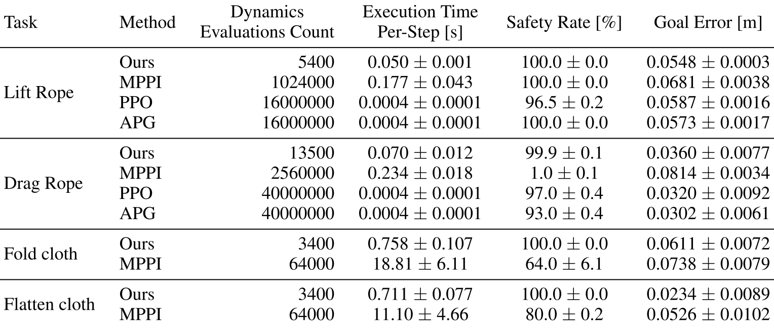
The experiments evaluate contact discovery, simulated safety/goal error, learning curves, output-feedback rollouts and hardware feasibility. Dynamics-evaluation counts, online planning time, offline training interactions and policy inference time have different meanings. Safety percentages in a benchmark do not substitute for verifying the formal assumptions. The complete tables retain results that favor other methods on selected accuracy, speed or goal metrics.
Accessible original table, complete values and grouped headers
| Task | Method |
|
|
Safety Rate [%] | Goal Error [m] | ||||
| Lift Rope | Ours | 5400 | 0.050 0.001 | 100.0 0.0 | 0.0548 0.0003 | ||||
| MPPI | 1024000 | 0.177 0.043 | 100.0 0.0 | 0.0681 0.0038 | |||||
| PPO | 16000000 | 0.0004 0.0001 | 96.5 0.2 | 0.0587 0.0016 | |||||
| APG | 16000000 | 0.0004 0.0001 | 100.0 0.0 | 0.0573 0.0017 | |||||
| Drag Rope | Ours | 13500 | 0.070 0.012 | 99.9 0.1 | 0.0360 0.0077 | ||||
| MPPI | 2560000 | 0.234 0.018 | 1.0 0.1 | 0.0814 0.0034 | |||||
| PPO | 40000000 | 0.0004 0.0001 | 97.0 0.4 | 0.0320 0.0092 | |||||
| APG | 40000000 | 0.0004 0.0001 | 93.0 0.4 | 0.0302 0.0061 | |||||
| Fold cloth | Ours | 3400 | 0.758 0.107 | 100.0 0.0 | 0.0611 0.0072 | ||||
| MPPI | 64000 | 18.81 6.11 | 64.0 6.1 | 0.0738 0.0079 | |||||
| Flatten cloth | Ours | 3400 | 0.711 0.077 | 100.0 0.0 | 0.0234 0.0089 | ||||
| MPPI | 64000 | 11.10 4.66 | 80.0 0.2 | 0.0526 0.0102 |
Simulation Benchmark Comparison
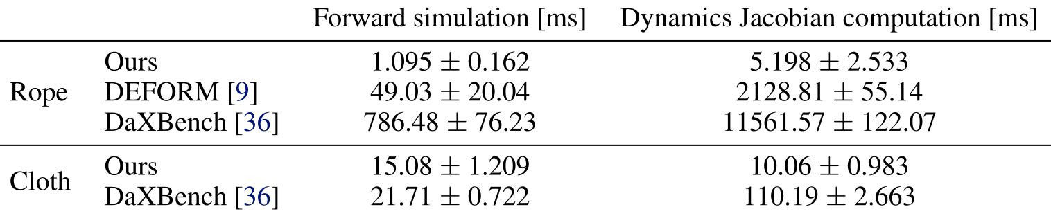
AppendixF compares forward/Jacobian runtimes for a 20-node rope and 100-node cloth, then evaluates settled hardware rope prediction using a different 10-link configuration. Maximum speedups are setting-specific: rope forward 1.095 ms versus DaXBench 786.48 ms is about 718×, while Jacobian 5.198 ms versus 11561.57 ms is about 2224×. Cloth speedups are much smaller. DEFORM has lower prediction error than CORD-SLS, so the speed benefit comes with a fidelity tradeoff rather than uniform accuracy superiority.
Original mathematical definitions, assumptions and evaluation protocol
See App. F for baseline comparisons of our differentiable simulator against prior simulators [9, 36] in terms of accuracy and runtime. We show that our simulator achieves comparable accuracy while accelerating forward simulation and Jacobian computation by up to 700 and 2000, respectively. This efficiency, along with the integration of contact smoothing, enables real-time control rates and low goal error in our deformable object planning experiments, which we discuss next.
Planning Benchmark Comparison on Deformable Manipulation Tasks
Table 1 gives rope planner times 50/70 ms versus MPPI 177/234 ms and cloth 758/711 ms versus 18.81/11.10 seconds. Learned policies infer in.4 ms, faster than the online planner. CORD-SLS reports 100/99.9/100/100% safety across lift/drag/fold/flatten, but drag PPO/APG achieve lower goal error at 97/93% safety. APG's cost improvement is not improved safety over PPO in that task. Cloth has no RL comparison. Different tasks need their own costs/constraints; the common optimizer's reuse is not an unchanged learned multitask policy. Rollout-count/uncertainty semantics for Table 1 are not fully specified, so no new significance claim is inferred.
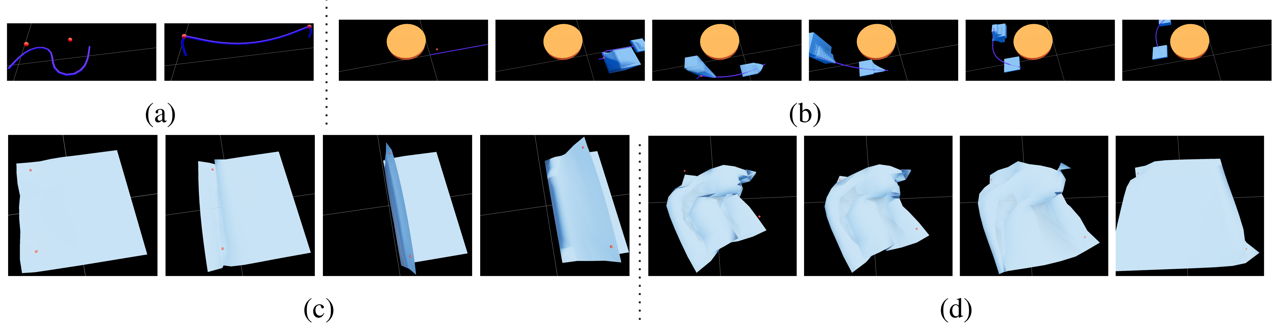
Original selectable panel captions and notation
(a)
(b)
(c)
(d)
Output Feedback
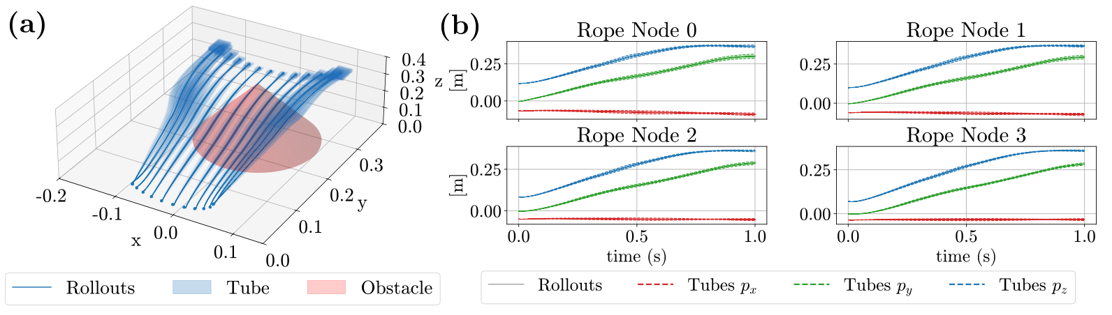
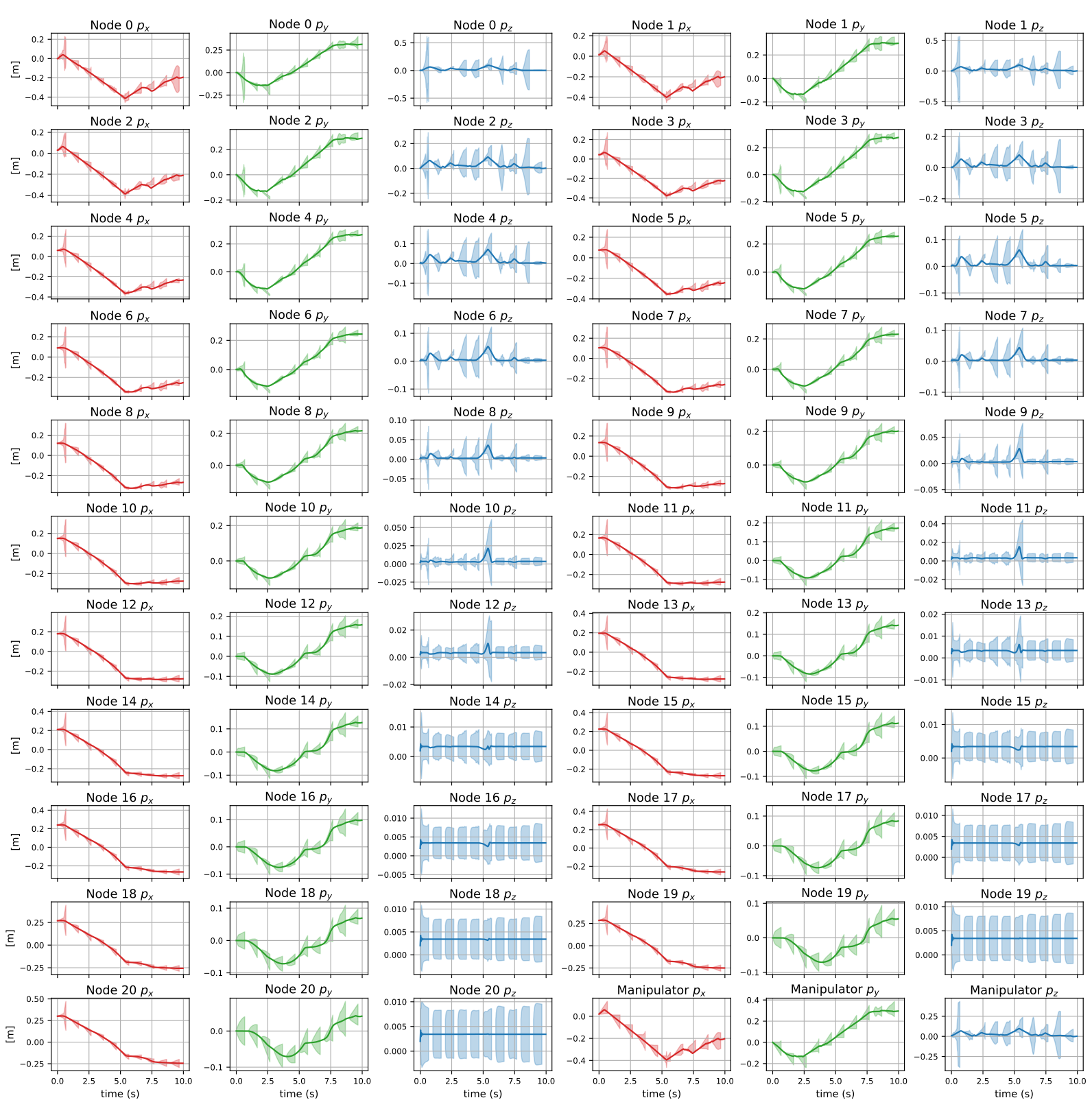
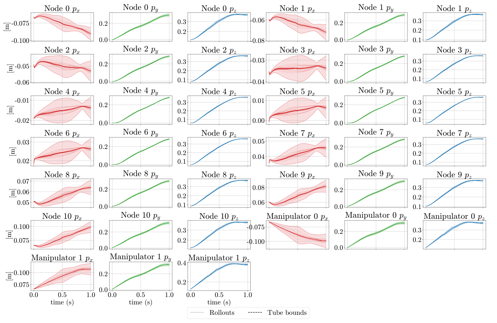
Figures 3/9 show output-feedback rope rollouts under simulated process and measurement disturbances, with the full 39-state tube grid retained. They illustrate containment for the synthesized finite-horizon observer/controller and sampled disturbances. This evidence differs from executing a sequence of newly replanned controllers or certifying unseen perception failures.
Hardware
Hardware uses two KUKA iiwa arms, RGB-D keypoint reconstruction and separate perception/solver GPUs. The paper collects 100 random-control transitions and chooses a rounded.03 m radius covering 87% of calibration residuals. That is empirical in-sample coverage, not the formal trajectory-level quantile guarantee. Two tasks demonstrate rope obstacle traversal and cloth folding; no repeated-trial success denominator or measured trajectory-level confidence is supplied. Four project movies are two views of these behaviors, not four independent statistical trials. Hardware solve time below 20 ms and slower perception differ from Table 1's benchmark timings.
6 Discussion, Limitations, and Conclusion
The useful contribution is an integrated fast simulator and robust-planning interface with a clear finite-horizon containment argument. Experimental results show feasible contact-rich rope/cloth control and favorable planning costs in selected settings. Conclusions about certified real-world safety remain conditional on calibration, full-state estimation error bounds, nonlinear tube validity and the actual controller used during the horizon.
Limitations
The paper identifies contact-smoothing error, occlusion/topology-sensitive perception and memory growth with state dimension/horizon as limitations. Proposed remedies—smoothing-error tubes, better sensing/learned observations and low-rank responses—are future or referenced extensions. The reported implementation does not thereby acquire these additional protections.
Original hardware recordings and interactive rollouts
All four original WebM hardware recordings are preserved locally with unchanged source bytes and derived poster frames. Side/front camera pairs depict rope and cloth behavior. Original interactive Viser simulations and the overview video remain linked at their source hosts; the edition does not claim local copies of those viewers. Interactive rollouts are simulation illustrations, while multiple camera views do not expand the hardware trial count.
Appendix A Proofs
Both the main theorem and its appendix restatement are preserved in full, together with the proof. The proof uses q=perceived-state minus measurement error: on a valid perceived-state containment event, adding the error ball contains the true state. It carries the assumed event's probability lower bound forward. It does not independently prove the antecedent SLS containment, exchangeability, a numeric hardwareρ bound or recursive feasibility. The two original proof displays remain alongside their selectable source.
Theorem A.1 (True-state containment from perceived-state conformal tubes).
Let with , and define . Suppose conformal calibration and robust SLS synthesis yield perceived-state and control tubes and satisfying . Then the true state and control trajectories satisfy .
Proof.
On the event that and for all , we have
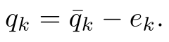
Original selectable mathematical display
Equation
Since ,

Original selectable mathematical display
Equation
for all . The perceived-state containment event has probability at least , so the inflated true-state containment event has the same probability lower bound. ∎
Appendix B Perception
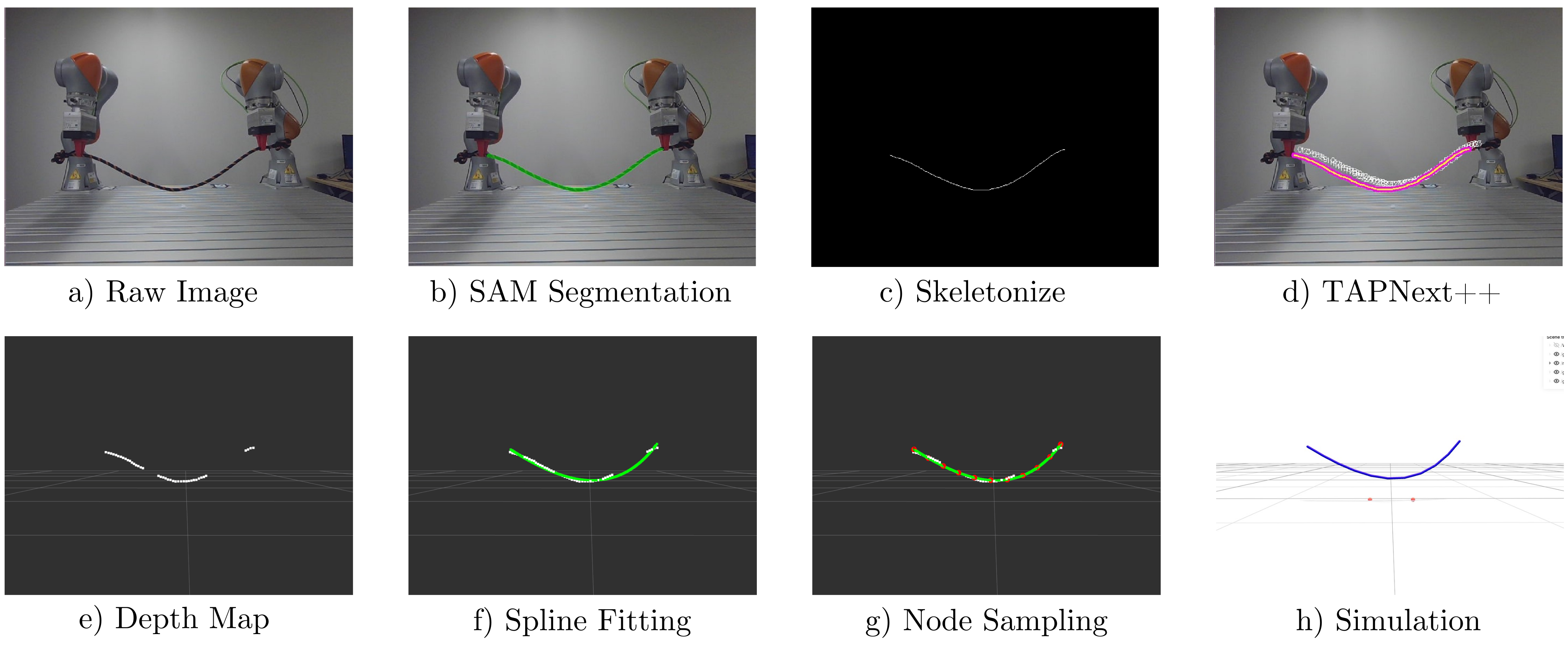
Two Orbbec Gemini 336 L cameras are calibrated to the robot workstation. An RTX4090 handles perception/robot communication and an RTX4070 Ti Super runs the solver, connected through ROS2/Ethernet. The visual state is reconstructed through segmentation, tracking, depth and structural assumptions, so camera specifications alone need not bound the entire reconstructed state. Both perception diagrams retain every panel.
B.1 Rope
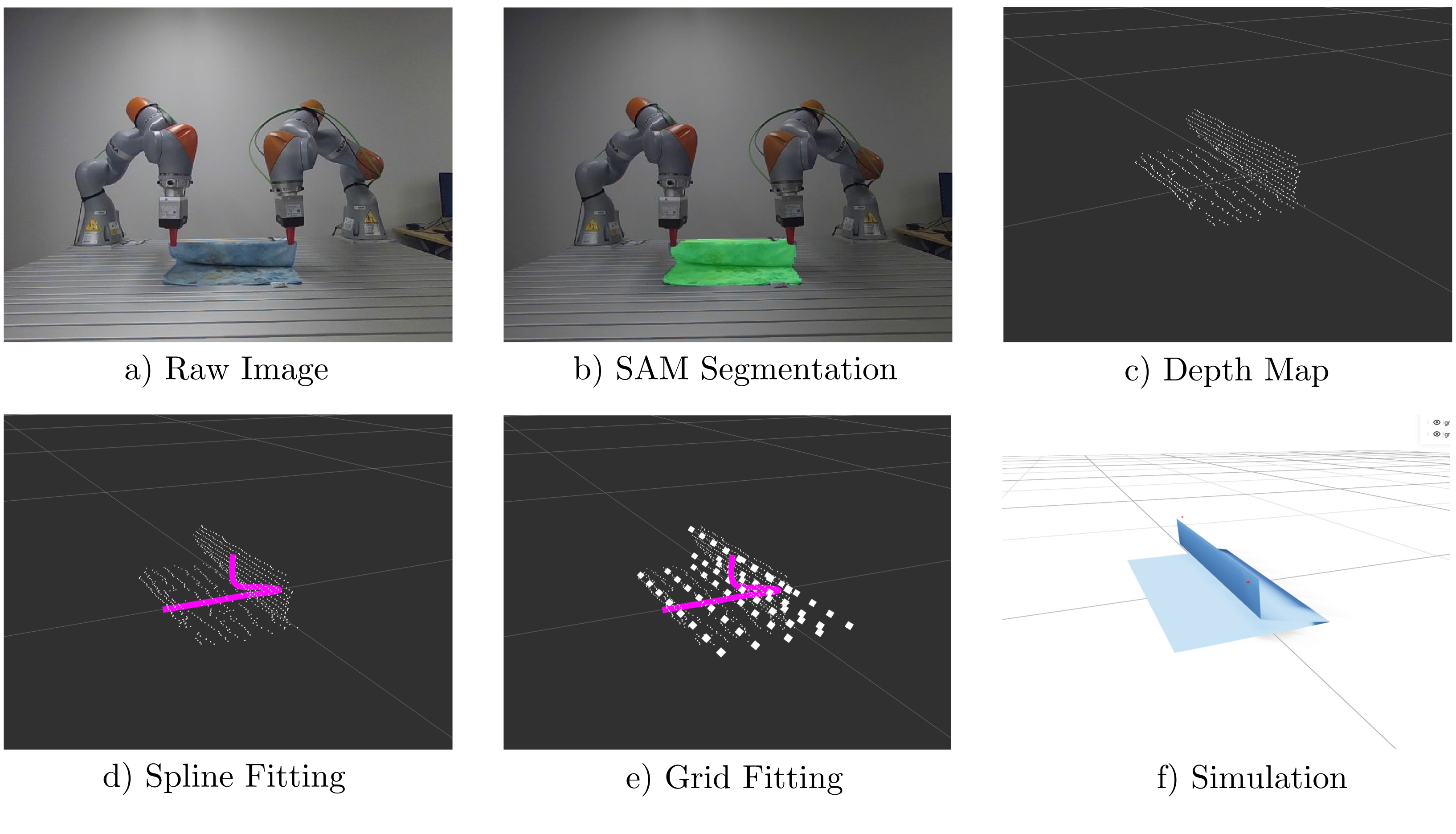
The braided rope is about 1 cm thick and 1.5 m long, tied to an effective.8 m span and modeled with 10 links on hardware. SAM3 with the rope prompt initializes/re-grounds a skeleton tracker; TAPNext++ tracks between updates, then depth/splines reconstruct ordered 3 D nodes. Re-grounding every 1/5 seconds gives roughly 15/25 Hz tracking, slower than the under 20 ms solver. A faster post-grasp reconstruction instead assumes gravitational sag from gripper poses and known length. Its speed benefit depends on that shape assumption and is distinct from continuously observing every node.
B.2 Cloth
The 38×38 cm cloth uses an 8×8 node lattice plus grippers for 198 state coordinates, unlike the 300-DoF simulation benchmark. Perception assumes each row is straight across cloth width, reconstructs a centerline/boundary spline and fills occluded geometry using known length. The optimization constrains gripper x/z differences within 5 cm to support this simplification. This task-specific prior makes folding tractable but limits claims about arbitrary wrinkles, topology or general occluded cloth estimation.
Original mathematical definitions, assumptions and evaluation protocol
We use an approximately 38 cm x 38 cm cloth. For our simulation model, the cloth is discretized into a 7 x 7 grid of cells, corresponding to an 8 x 8 lattice of nodes and yielding 64 cloth nodes in total. The full state has dimension (), consisting of the 3D positions of the cloth nodes and two 3D gripper positions.
Appendix C RL training convergence
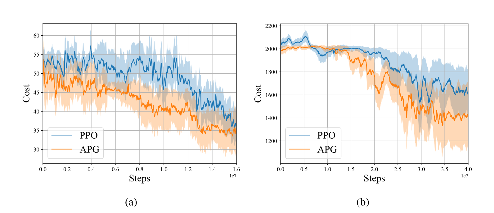
APG reaches PPO's cost with mean 45.95% fewer steps for lifting and 16.63% fewer for dragging; reported medians 36.01/27.43% use a different summary. These are training-curve cost-matching comparisons, not faster online policy inference or guaranteed safe learned behavior. The main table's fixed interaction budgets remain alongside the convergence plots and their uncertainty bands.
Original selectable panel captions and notation
(a)
(b)
Appendix D State Feedback MPC Tubes
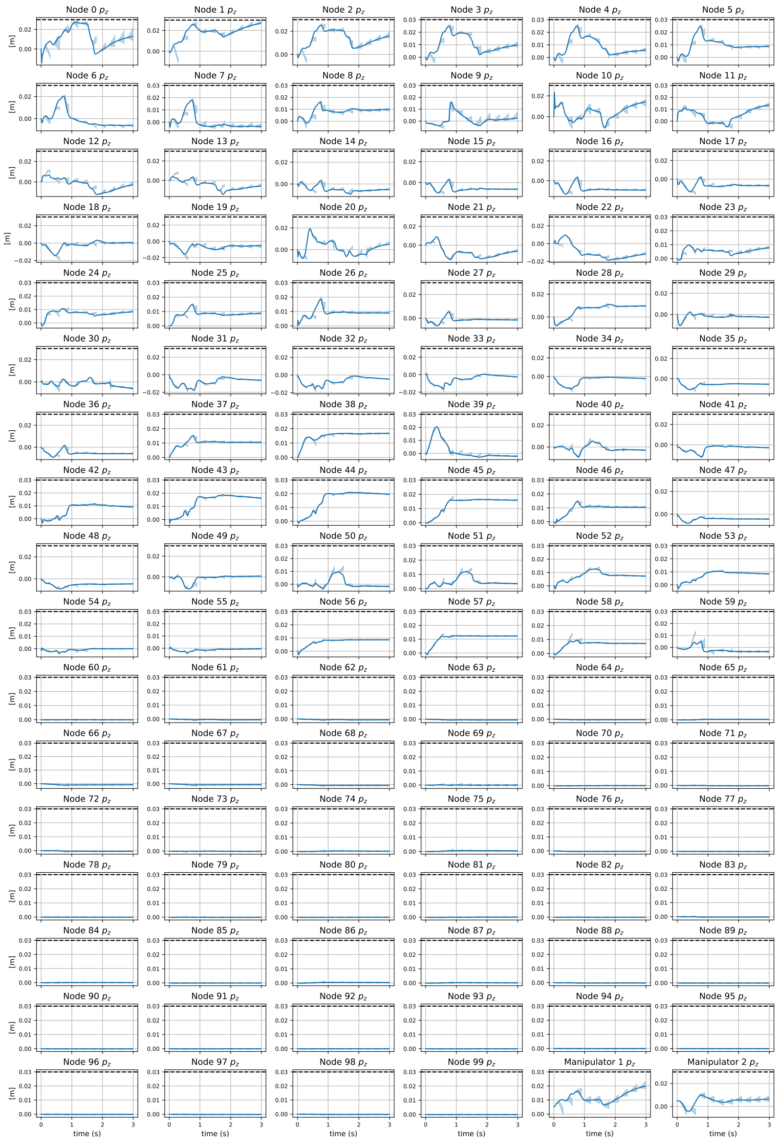
Figure 7 retains all 66 rope-state plots and Figure 8 the full cloth z-coordinate grid. The text explicitly warns that repeatedly replanned execution can leave tubes computed at earlier steps: the controller and future path have changed. Keeping a previously synthesized robust feedback controller gives containment over its own finite horizon, while guaranteed robust recursive feasibility needs an additional approach such as the cited disturbance-feedback MPC. Replanning alone is not a proof that every old tube remains valid. The cloth example's 3 cm height constraint is the particular task constraint, not a global guarantee for arbitrary folding.
Original mathematical definitions, assumptions and evaluation protocol
Fig. 8 shows the forward reachable tubes for the fold cloth task in Fig. 2(c) at selected MPC steps. A constraint limits the cloth height to 3 cm in the direction. Because MPC replans after each execution step, the executed trajectory does not necessarily remain within tubes computed at previous time steps. Nevertheless, by enforcing constraints on the tube-valued predictions during each replan, the controller robustly satisfies the -height constraint throughout the task.
Appendix E Output Feedback Tubes
The complete 39-state output-feedback grid shows rollouts using the synthesized observer-based controller under randomized dynamics/measurement disturbances. These fixed-controller finite-horizon plots should be read separately from AppendixD's receding-horizon overlays. Colors denote coordinate directions; the native vector export preserves every bound, label and curve.
Appendix F Simulator Comparison
Runtime Table 2 uses 20-node rope/100-node cloth and favors the GPU-native implementation, while the compared DEFORM pipeline is not compiled into GPU-native code. Accuracy Table 3 uses 100 settled hardware transitions,70/30 residual-model train/validation split and 10 links. Latency prevents observing transient swinging; DEFORM is advanced to equilibrium before comparison. Raw mean errors are.0150 m CORD-SLS versus.0139 m DEFORM, and residual-corrected.0075 versus.0071 m. Identical residual architectures reduce one confound, but the small settled-data study does not validate dynamic accuracy. Stretch/bend-only modeling differs from DEFORM's twisting mechanics, and finite differences in runtime/accuracy do not establish universal dominance.
Accessible original table, complete values and grouped headers
| Forward simulation [ms] | Dynamics Jacobian computation [ms] | ||
| Rope | Ours | 1.095 0.162 | 5.198 2.533 |
| DEFORM [9] | 49.03 20.04 | 2128.81 55.14 | |
| DaXBench [36] | 786.48 76.23 | 11561.57 122.07 | |
| Cloth | Ours | 15.08 1.209 | 10.06 0.983 |
| DaXBench [36] | 21.71 0.722 | 110.19 2.663 |
Original mathematical definitions, assumptions and evaluation protocol
We next benchmark the simulation accuracy of our method against DEFORM. To construct the benchmark dataset, we collect 100 samples of randomized manipulation actions on hardware while running our perception pipeline to estimate the rope state. For each sample, we record the current state, control action, and resulting next state, i.e. (). We note that due to the latency in the perception pipeline, we are unable to directly observe the instantaneous post-action state and therefore cannot reliably capture transient swinging or momentum-driven dynamics. Instead, the recorded next state corresponds to the settled configuration of the rope after the motion has dissipated, making the dataset more representative of quasi-static behavior.
