At a glance
The paper studies polynomial point-robot trajectories among spherical obstacles, with derivative costs and boundary/continuity constraints. Exact sum-of-squares collision certificates lead to a semidefinite relaxation whose slack has a geometric meaning: it permits motion in extra dimensions. This characterizes tightness and supports a smaller, symmetry-reduced formulation. Experiments show much faster, more consistent solves than the tested nonlinear baselines and useful RRT steering. A loose relaxation can project through obstacles; global optimality of the original trajectory requires the stated tightness and recovery conditions.
I Introduction
Collision avoidance remains nonconvex even for a point robot, while smoothness and boundary constraints complicate geometric planning. The approach combines exact whole-curve collision certificates with a first-order convex relaxation, then uses sampling to supply global exploration. Unlike time-sampled collision constraints, the certificate covers every point on a fixed polynomial segment. The theoretical contribution explains when lifting preserves the original optimum and when extra-dimensional shortcuts make it loose, building on the SOS/moment framework.
II Related Works
Prior work applied moment/Shor relaxations to dynamics, collision avoidance, time scaling and contact, often observing tightness empirically. This paper deliberately restricts geometry and cost to analyze tightness rather than assume it. Its symmetry reduction addresses ambient-coordinate redundancy and can coexist with sparsity across trajectory segments. The analyzed setting does not encompass arbitrary articulated robots or general nonlinear dynamics.
III Motion Planning
The initial problem optimizes a continuously differentiable curve, with obstacle inequalities required at every parameter value. Restricting to finitely many polynomial coefficients gives a finite-dimensional decision variable but leaves infinitely many collision constraints. The SOS construction removes those continuum constraints exactly within the selected polynomial class.
III-A Problem Statement
Minimize the integral of the squared kth derivative over [0,1], subject to Cη continuity, prescribed endpoint derivatives through order ℓ, and distance at least each obstacle radius. Examples are velocity/energy, acceleration and snap costs. Exactness later refers to this polynomial, fixed-parameter-domain formulation, not automatically the unrestricted infinite-dimensional or free-time optimum.
Equations 1a–1f
| (1a) | ||||
| (1b) | ||||
| (1c) | ||||
| (1d) | ||||
| (1e) | ||||
| (1f) | ||||
III-B Polynomial Curves
A segment is γ(s)=Γbᵈ(s), with coefficient matrix Γ of size n×(d+1). Costs and obstacle conditions separate by segment; linear derivative-matching constraints couple neighboring segments. Derivations are mostly basis-independent, with Bernstein/Bézier coordinates used in the implementation.
Equation 2
| (2) |
III-C Curve Costs
Squared derivative cost is tr(G⁽ᵏ⁾ΓᵀΓ), where the derivative Gram matrix is analytic for a chosen basis. Its rank is d+1−k and its nullspace consists of polynomials below degree k. These zero-cost directions explain why endpoint conditions matter for uniqueness.
Equations 3–5
| (3) |
| (4) |
| (5) |
III-D Semi-Infinite QCQP Reformulation
For a unit sphere, squared distance minus one is a univariate polynomial of degree at most 2d. A coefficient vector u represents the constant polynomial one, giving the shifted matrix Γ−cuᵀ. The resulting problem has quadratic cost/obstacle terms and linear boundary equation ΓA=B, but still requires polynomial nonnegativity for every s.
Equations 6–9
| (6) |
| (7) | ||||
| (8) | ||||
| (9) |
IV Certifying Collision-Avoidance
A univariate polynomial’s nonnegativity on an interval has an exact SOS representation. Certifying a fixed path is convex; searching its coefficients remains nonconvex because the certificate depends quadratically on Γ.
IV-A Basis-Independent Derivation
Markov–Lukács writes an interval-nonnegative degree-2d polynomial as σ₀+(s−a)(b−s)σ₁, with SOS degrees at most 2d and 2d−2. Coefficient matching yields PSD Gram matrices of sizes d+1 and d, independent of ambient dimension n. The same fixed-curve certificate extends to ellipsoids through (Γ−cuᵀ)ᵀE(Γ−cuᵀ). The later geometric tightness analysis concerns spherical obstacles, not a proved general ellipsoid-planning theorem.
Equations 10–12
| (10) |
| (11) |
| (12) |
IV-B Collision-Avoidance with Bézier Curves
Dropping binomial factors gives a scaled Bernstein basis whose products simply add indices. The map S sums matrix antidiagonals; T shifts the degree-(d−1) map to account for s(1−s). Their coefficient identity is an exact collision certificate. The implementation uses standard Bernstein coordinates for conditioning, with weighted maps supplied in the appendix.
Equations 13–16
| (13) |
| (14) |
| (15) |
| (16) |
IV-C The Special Case of Line Segments
For a line segment, eliminating one SOS matrix leaves a 2×2 PSD condition and a nonnegative scalar α, expressible as a rotated second-order cone. This reduces certificate cost; joint optimization of segment endpoints still contains their nonconvex quadratic geometry before relaxation.
Equations 17–18
| (17) |
| (18) |
V Semidefinite Relaxation
The exact finite-dimensional problem and its convex relaxation differ at the coefficient Gram-matrix equality.
V-A Nonconvex Problem
Replacing continuum collision constraints by SOS coefficient matching produces a finite problem over Γ,Q₀,Q₁. The SOS matrices are PSD, but coefficient matching is quadratic in Γ, so exact reformulation alone has not convexified planning.
Equation P
| (P) | ||||
V-B Forming the Relaxation
Introduce X=ΓᵀΓ to make cost and collision matching affine, then relax equality to X⪰ΓᵀΓ through a Schur-complement block LMI. The implied relation XA=ΓᵀB tightens the relaxation and is essential for the lifted path’s endpoint conditions. The collision-certificate cones have sizes d+1 and d; the displayed joint Schur block is n+d+1, so the entire numerical formulation is not literally independent of n.
V-C Strict Feasibility and Facial Reduction
Boundary and tightening equations force the feasible set into a proper PSD-cone face, preventing strict feasibility in the unreduced form. In Bernstein coordinates, endpoint derivatives fix adjacent control points, allowing explicit elimination. With independent endpoint conditions, d+1−2(ℓ+1) free control points remain for a single segment, reducing the Schur block and removing known degeneracy.
Equation
V-D Extension to Multiple Segments
Multiple segments introduce within-segment and adjacent cross-Gram matrices. Cη matching supplies linear coefficient constraints and implied Gram constraints; these also permit facial reduction. The interior pairwise Schur block shrinks by η+1 columns, with further endpoint reductions. This preserves coupled smoothness rather than optimizing disconnected curves.
Equations 21
| (21) |
VI Theoretical Results
The main results interpret positive slack as real motion in extra dimensions, characterize equality of optimum costs, and distinguish cost tightness from recovery of a particular path.
VI-A Geometric Interpretation
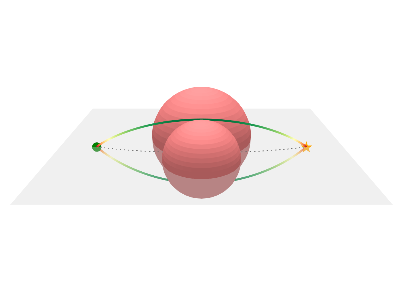
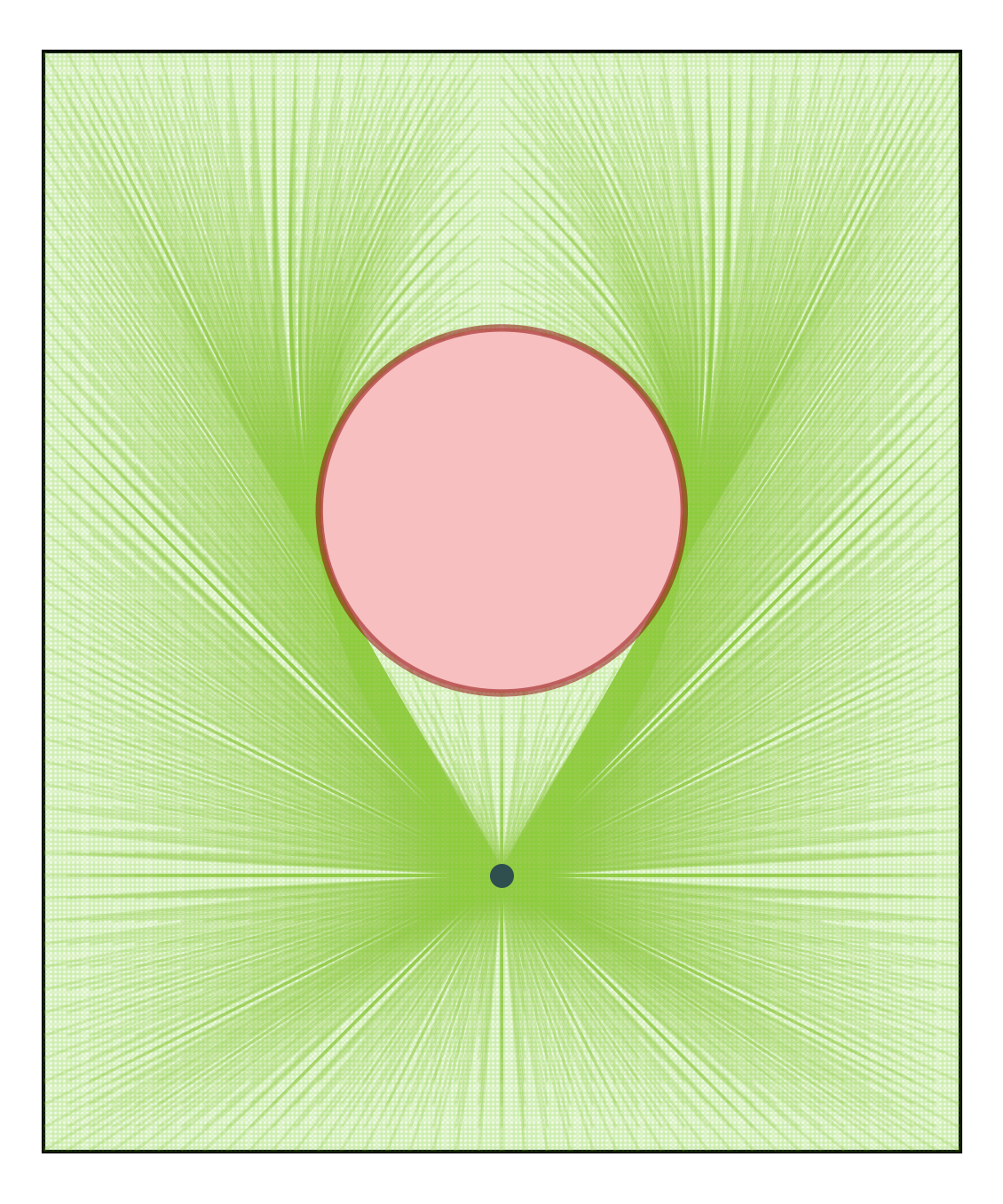
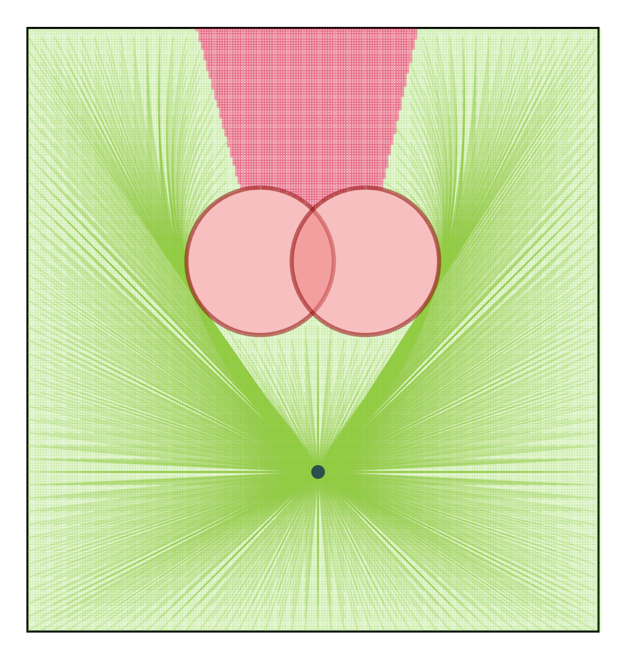
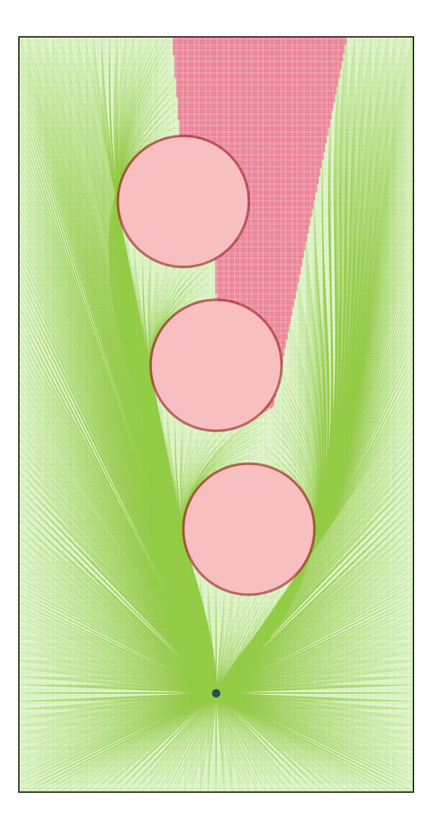
Factor the slack as VᵀV=X−ΓᵀΓ. The lifted trajectory (Γbᵈ,Vbᵈ) avoids spheres centered at (c,0), with V and its prescribed endpoint derivatives zero. Increasing the number ρ of extra dimensions cannot increase optimal cost; the SDP lower-bounds every lifted problem and attains one of them at ρ=rank(X−ΓᵀΓ). Thus it solves the cheapest member of that family. Independent boundary conditions bound ρ by the number of free control points. Only ρ=0 or 1 appeared in the reported experiments; a universal one-dimension bound is not proved.
Equation P ρ
| (Pρ) | ||||
VI-B When is the Relaxation Tight?
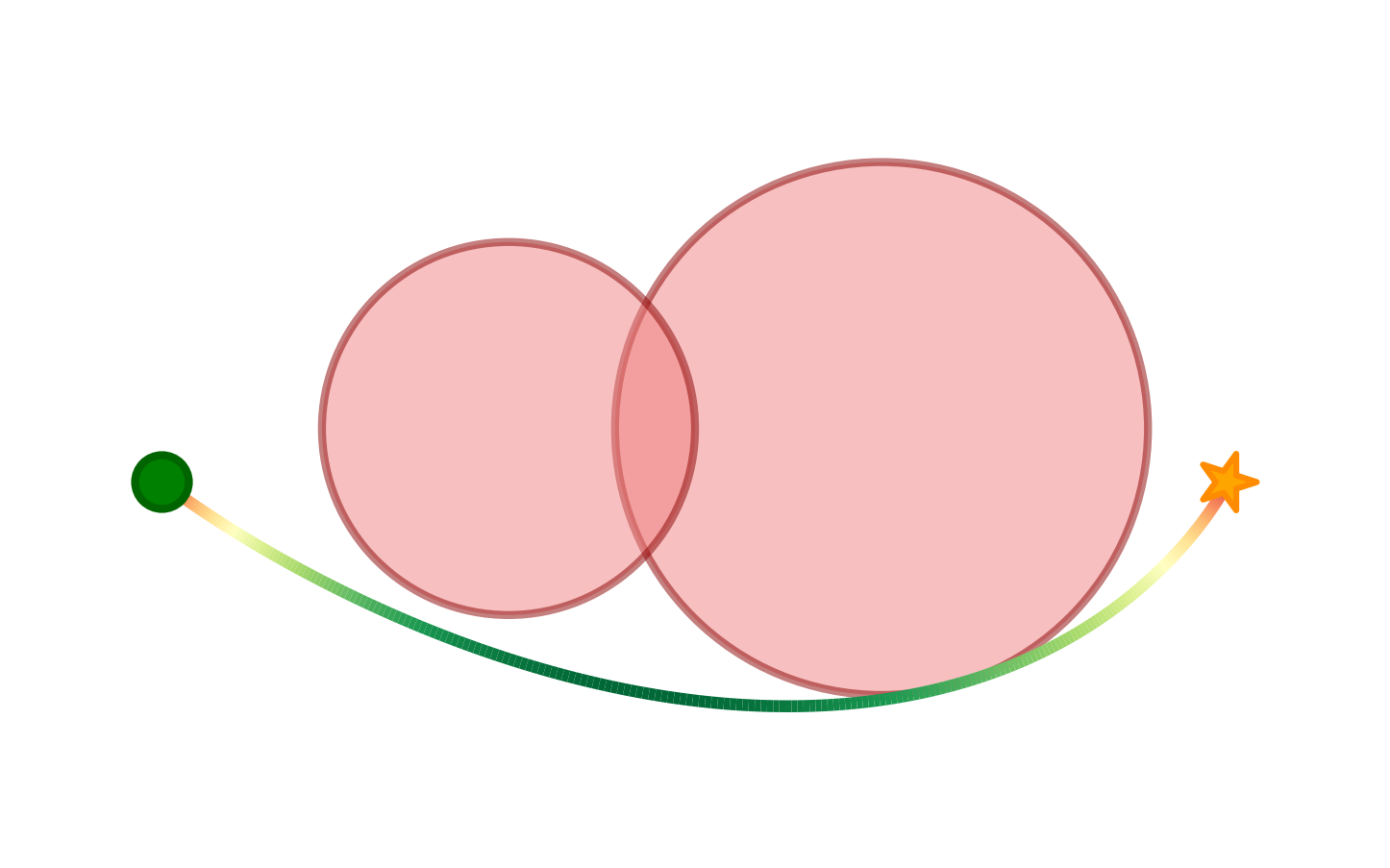
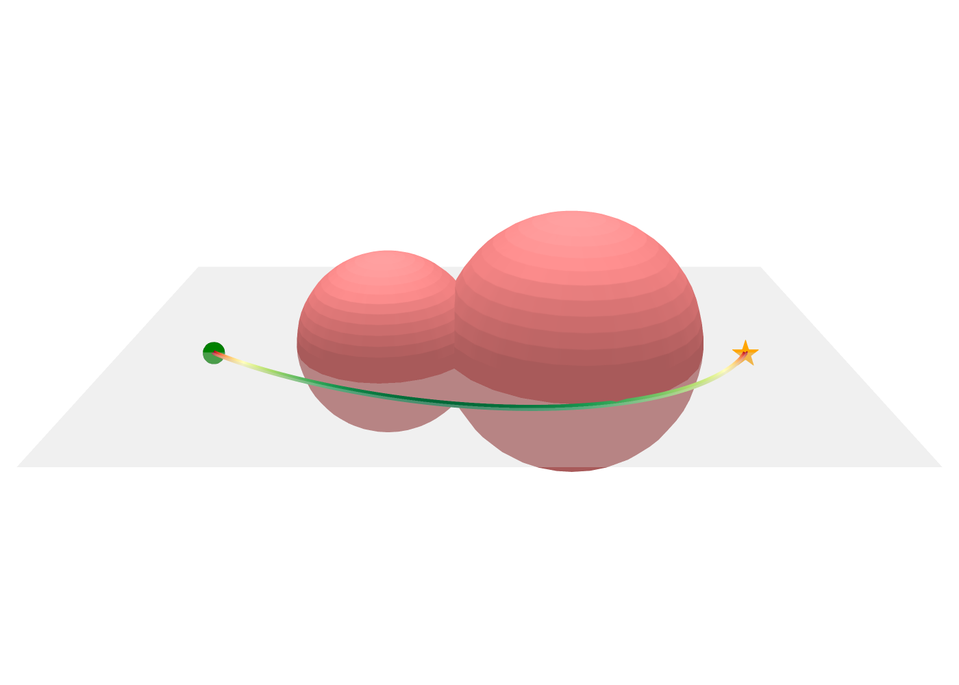
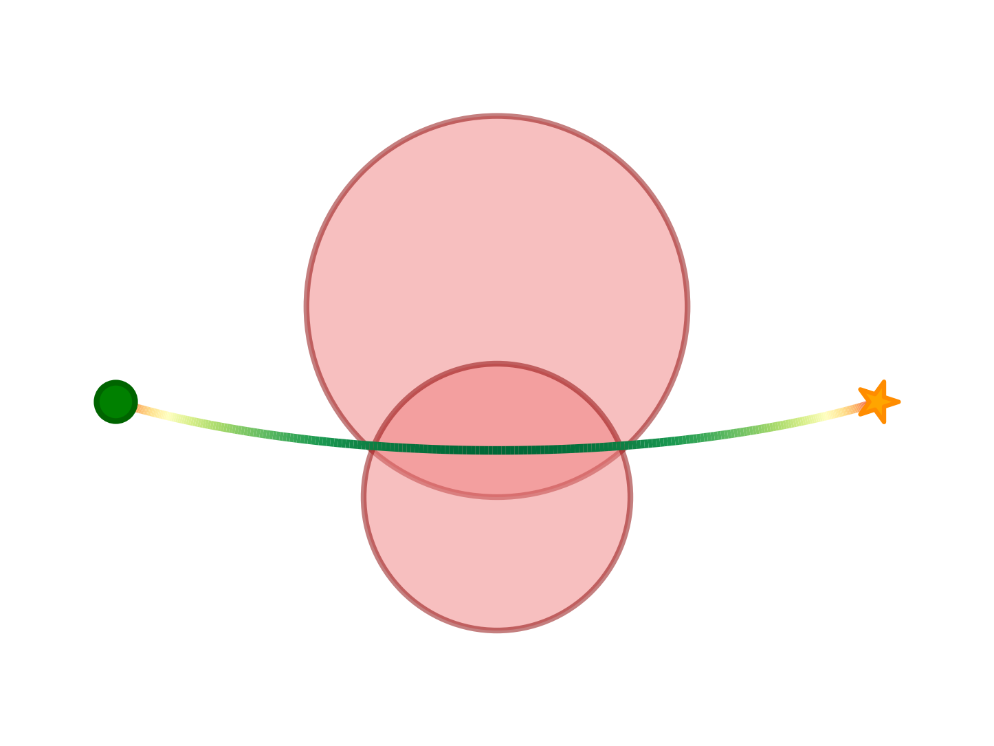
Theorem 4 states that the SDP has the original optimal cost exactly when no number of extra dimensions permits a cheaper feasible path. This gives a geometric characterization, not a guarantee that an arbitrary environment is tight. Figure 2 contrasts a genuine planar optimum with a lifted shortcut whose planar projection collides.
VI-C Recovering a Minimizer
Theorem 5 adds a stronger recovery condition: every optimum of every lifted problem must have the same Γ and V=0. Then every SDP optimum recovers that path and X=ΓᵀΓ. Cost tightness alone need not identify a unique trajectory. Endpoint conditions eliminate derivative-cost null directions when k≤2(ℓ+1); obstacle symmetry can still create distinct equal-cost routes. Small geometric perturbations often remove that symmetry in practice.
VII Empirical Analysis
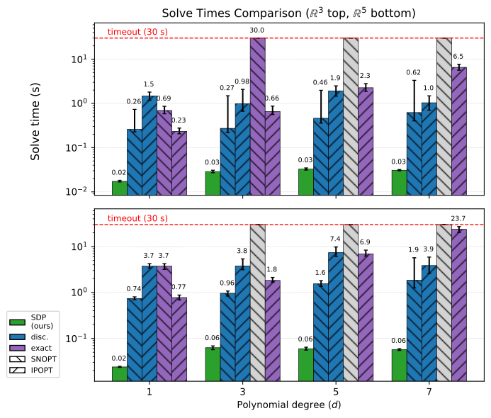
Random comparisons use 100 instances in R³ with fifteen obstacles and R⁵ with thirty, radii 0.3–1.0 in [−2,2]ⁿ. Nonlinear baselines use either twenty collision samples per segment or the exact SOS condition with PSD matrices factorized as LLᵀ. SNOPT/IPOPT start from a straight line, use feasibility tolerance 10⁻⁴ and a thirty-second timeout. All methods receive analogous equality-variable reduction. Table I varies degrees 1/3/5/7, derivative costs, continuity and segment counts; results depend on this setup.
| Degree | Cost | Continuity | BC | Segments |
|---|---|---|---|---|
| 1 | velocity () | 0 | 12 | |
| 3 | acceleration () | 2 | 6 | |
| 5 | jerk () | 3 | 4 | |
| 7 | snap () | 4 | 3 |
VII-A Computational Cost
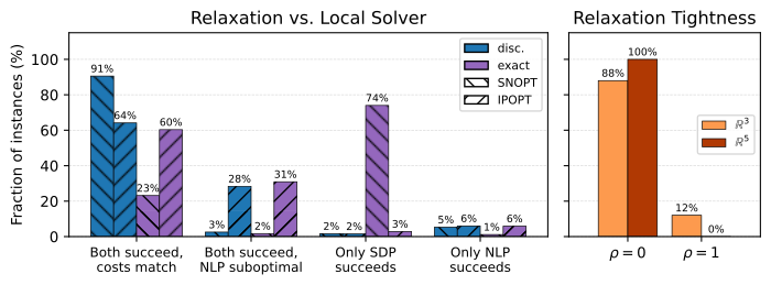
SDP median solves are 17–33 ms in R³ and 24–63 ms in R⁵; interquartile ranges are 1–4 and 1–12 ms. The sampled nonlinear baselines are generally tens of times slower, while exact nonlinear transcriptions can time out or become hundreds of times slower. Figure 4 retains the detailed ratios, including 212×/397× versus exact IPOPT at degree seven. Timed-out instances are excluded from the quoted nonlinear spread statistics, and an interquartile range should not be read as a formal variance estimate.
VII-B Empirical Tightness
Against the strongest baseline, 91% of the selected comparison instances have matching successful costs; the denominator includes only cases where the relaxation is tight or the baseline succeeds. It is not an unconditional 91% success rate. Figure 4 reports 88% rank-zero and 12% rank-one slack in R³, and 100% rank-zero in R⁵. The relationship between tightness and successful local optimization is empirical; loose cases still need global exploration or refinement.
VIII Kinodynamic Motion Planning
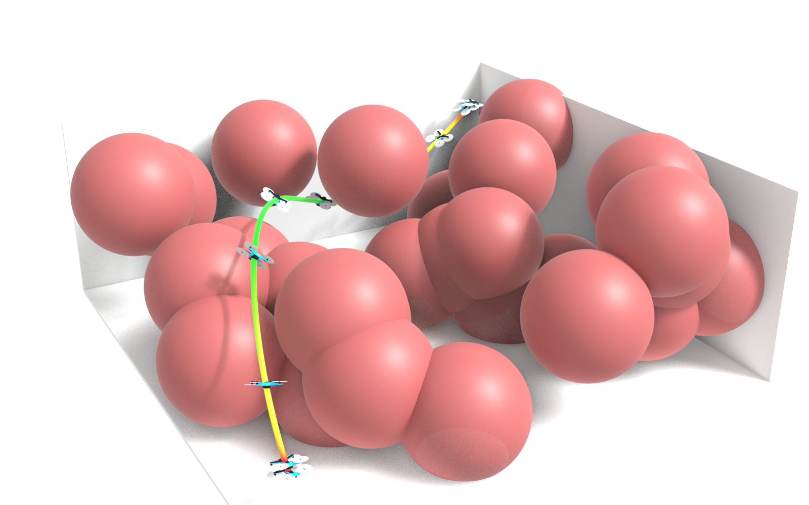
The relaxation supplies steering inside an RRT for degree-nine, C⁴-continuous minimum-snap trajectories. Convex steering can optimize smoothness and compatible convex trajectory constraints, while the sampler explores alternatives. A relaxation solve by itself is a collision-free original-space solution only when recovery/feasibility checks succeed; the paper’s earlier loose examples preclude an unconditional claim for every solve.
VIII-A RRT Implementation
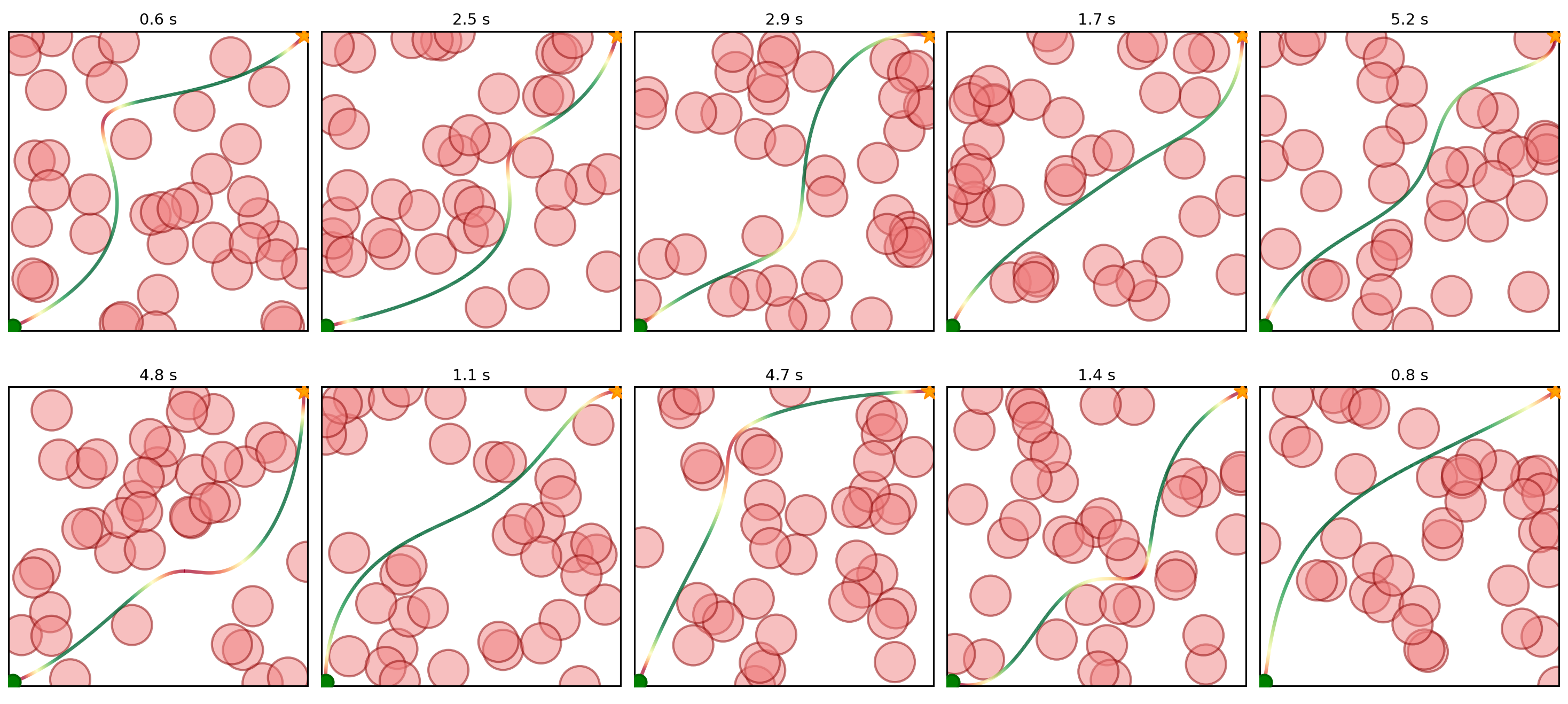
SDP-RRT and NLP-RRT sample positions with endpoint derivatives left free; Geometric RRT finds waypoints before nonlinear smoothing. The nonlinear steering baseline uses smoothed signed-distance constraints, inflated obstacles, reduced collision sampling, adjusted tolerances and solver switching. SDP-RRT jointly reoptimizes the last two segments on each extension to control derivative growth, fixing derivatives when reaching the goal.
VIII-B Trajectory Post-Processing
SDP refinement adds sampled separating cuts between trajectory points and obstacles, resolves, and repeats until collision-free, then resamples to reduce cost. Once dense cuts make SOS constraints largely inactive, those constraints are dropped and each iteration becomes a small convex QP. This is explicitly heuristic post-processing; the exact whole-curve guarantee of the original SOS formulation should not be transferred to arbitrary sampled cuts without the stated collision verification.
VIII-C Numerical Results
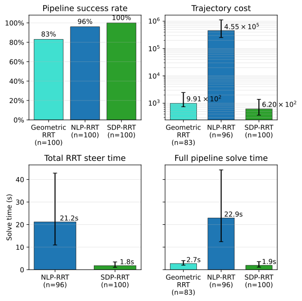
On 100 planar environments with forty radius-one obstacles in a 15×15 square, SDP-RRT succeeds in 100 runs, NLP-RRT in 96 and geometric-plus-smoothing in 83. Median full times are 1.9, 22.9 and 2.7 seconds; median trajectory costs are 620, 455,000 and 991, respectively. Costs/times use each method’s successful runs, so their subsets differ. SDP steering totals 1.8 seconds versus 21.2 for NLP, excluding program-construction overhead. This benchmark has no extra dynamic or input bounds: support for such convex constraints is a capability of the formulation, not quantitatively demonstrated here.
IX Conclusion
The relaxation is useful as a fast local component, yet can be loose where global routing matters. Open directions include higher-order moment relaxations, tighter slack-rank bounds, richer polynomial geometry, additional convex dynamics/input constraints and a structure-specialized solver. The evidence does not claim globally optimal arbitrary-robot motion planning or physical quadrotor deployment.
-A Connection To the Shor Relaxation
Vectorized Shor lifting uses Y⪰yyᵀ for y=vec(Γ), a matrix of size n(d+1). Decompose Y=yyᵀ+S: cost and collision equations depend on slack S only through blockwise partial traces. Orthogonal conjugation of each n×n block preserves feasibility and objective. Averaging over this symmetry restricts slack to S=(1/n)Λ⊗Iₙ, reducing its free PSD variable to size d+1. Substituting X=ΓᵀΓ+Λ recovers the proposed relaxation with tightening constraints. This is a symmetry of the slack construction, not an assumption that obstacle locations are rotationally symmetric.
Equations 22–24
| (22) |
| (Shor) | ||||
| (Shor′) | ||||
| (23) |
| (24) |
-B Proofs for the Theoretical Results
Theorem 1 pads a lifted path with a zero coordinate. Theorem 2 projects the lifted SDP onto (Γ,X), or extends it with V=0, showing the same convex lower bound. Theorem 3 factors positive slack and uses XA=ΓᵀB together with ΓA=B to prove VA=0; the constructed path attains the bound. Lemma 4 bounds rank through the boundary matrix’s nullspace. Theorem 4 follows from both cost inequalities. Theorem 5 rules out nonzero slack because it would produce a forbidden lifted optimum under its uniqueness hypothesis. These are conditional exact results for the stated problem, not a proof that sampled experiments are always tight.
-C Proofs for Symmetry Reduction
Orthogonal congruence preserves PSD slack, its block traces and the implied boundary equation. A block invariant under every orthogonal conjugation must be a scalar multiple of the identity, yielding the fixed-point form. Its eigenvalues repeat n times, so S⪰0 is equivalent to Λ⪰0. Substitution then recovers every proposed SDP constraint and its objective, proving the reduction without changing optimal cost.
-D Bézier Curves and the Bernstein Basis
The implementation uses standard Bernstein polynomials, restoring the binomial factors omitted in the simpler main derivation. Product and s(1−s) identities translate between degrees; all original identities are retained.
Equations 25–27
| (25) |
| (26) | ||||
| (27) |
-D 1 Curve Costs for Bézier Curves
Repeated forward differences and the factor d!/(d−k)! give Bézier derivatives. Integrating Bernstein products gives an analytic Gram matrix; sandwiching it by the difference operators and the squared factorial factor produces G⁽ᵏ⁾. This avoids numerical quadrature for the derivative objective.
Equations 28–30
| (28) |
| (29) |
| (30) |
-D 2 Collision Avoidance for Bézier Curves
Partition of unity makes u the all-ones vector. In standard Bernstein coordinates, antidiagonal sums gain ratios of binomial coefficients, and the shifted map gains k(2d−k)/(2d(2d−1)). These weighted maps implement the same exact interval collision certificate.
Equations 31–33
| (31) |
| (32) |
| (33) |
Acknowledgement
Support is credited to NSF’s HAND engineering research center, three Amazon awards, and the Aker Scholarship. The original funding statement distinguishes the authors’ conclusions from those of the funders.