Overview
Code repository. This edition follows the complete twenty-eight-page, 7 November 2026 v2, including the full appendices. The PDF labels the last plot page as Figure 6 continued; the HTML calls it Figure 7. Both plot pages are retained.
At a glance
The paper makes full-update conic-solver iterations trainable at larger scales. A matrix-free adjoint differentiates each linear solve without constructing dense matrix derivatives; a spectral divided-difference rule stabilizes gradients through positive-semidefinite projection. Small learned penalty policies then reduce iterations on seven problem families and accelerate selected planning and batched workloads. Results target moderate accuracy and specific trained families; GPU throughput, solver iteration counts and closed-loop control performance remain distinct measures.
1 Introduction
Deep unfolding retains an optimizer’s update structure while learning components such as initialization and step parameters. It optimizes progress within a finite computation budget rather than learning an arbitrary replacement update. Earlier warm starts, parameter schedules, distributed quadratic solvers and Deep FlexQP motivate the approach.
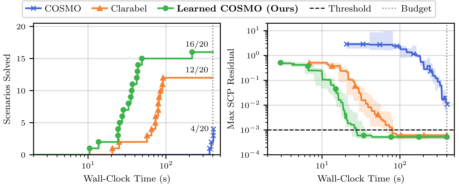
For large semidefinite programs, dense linear-solve derivatives consume memory and separate eigenvector derivatives become unstable at repeated eigenvalues. The contribution removes these training bottlenecks while retaining full COSMO updates. The reported control experiment solves 16/20 nonlinear covariance-steering scenarios, versus 4/20 baseline COSMO and 12/20 Clarabel; this is simulated optimization/control evidence, not robot-hardware validation.
2 Methodology
The method differentiates two internal operations of COSMO: a quadratic linear-system update and projection onto a product of cones. The rules could apply to related ADMM solvers with the same operations, but the experiments implement COSMO.
2.1 Deep Unfolding Conic Optimization
A convex quadratic objective is constrained by Ax+s=b with slack in a product of nonnegative, second-order and semidefinite cones. Learned maps choose solver parameters and optionally the starting iterate. Training backpropagates through K iterations to improve a trajectory-level loss; it differentiates the algorithm’s finite trajectory, not just its converged optimal solution.
Equations 1–2
| (1) |
| (2) |
2.2 Conic Operator Splitting Method (COSMO)
Each COSMO step solves a coupled quadratic system, relaxes the primal/slack iterates, projects the slack and updates the dual. The learned outputs are positive penalties and relaxation in (0,2); σ remains 10⁻⁶. Most operations use ordinary automatic differentiation, while the solve and PSD projection use custom rules. Valid parameter ranges alone do not establish convergence of every arbitrary state-dependent learned schedule.
Equations 3a–3e
| (3a) | ||||
| (3b) | ||||
| (3c) | ||||
| (3d) | ||||
| (3e) | ||||
2.3 Matrix-Free Implicit Differentiation
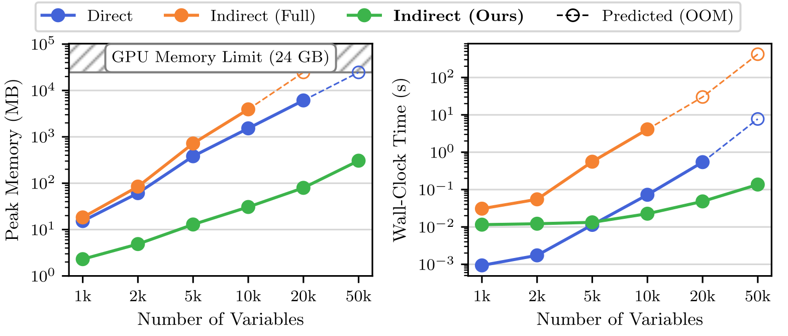
Eliminating the saddle-point multiplier gives a positive-definite system with operator P+σI+AᵀD(ρ)A. Conjugate gradients apply this operator through sparse matrix-vector products. For the backward pass, one adjoint solve with the same operator gives the gradient through its coefficient matrix; the right-hand-side gradient is returned separately so ordinary autograd includes its additional dependence on ρ. Omitting either path would give an incomplete derivative.
The algebra is exact for exact solves; finite forward/adjoint CG tolerances introduce numerical approximation. Avoiding dense AᵀA and its derivative saves memory, but total storage still includes sparse P and A and primal/constraint vectors. O(n+nnz(A)) is not automatically linear in n when sparsity density stays fixed, and runtime also depends on conditioning and CG iterations.
Equations 4–6
| (4) |
| (5) |
| (6) |
Equations
2.4 Stable PSD Projection
PSD projection clamps negative eigenvalues while preserving eigenvectors. Differentiating eigenvectors separately introduces reciprocal eigenvalue gaps; these can fail numerically even when the composed spectral projection has a well-behaved derivative.
The Dalečkii–Krein matrix-function rule, also used in DeepKSPD, forms divided differences of the clamping function and reuses the forward eigendecomposition. Repeated nonzero eigenvalues have finite limits. At zero the projection is nonsmooth: choosing the ReLU convention f′(0)=0 supplies a backward convention, not a classical Fréchet derivative valid in every perturbation direction.
Equations 7–10
| (7) |
| (8) |
| (9) |
| (10) |
Alternative Approaches.
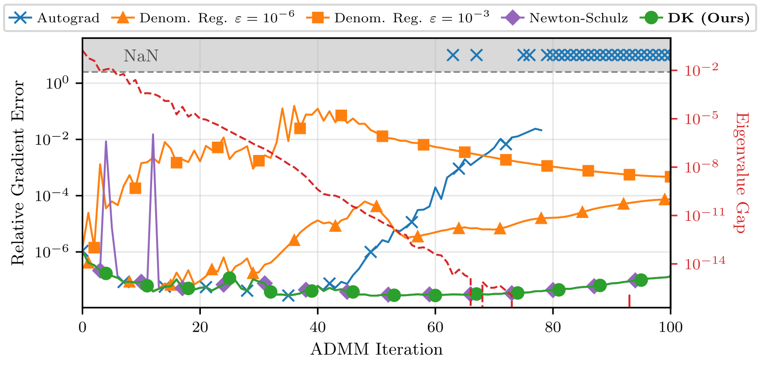
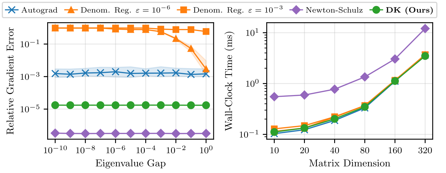
Denominator regularization avoids division by a zero eigenvalue gap but biases gradients when within-cluster gaps are small. Its zero output at an exact tie does not generally reproduce the DK off-diagonal limit, even as regularization vanishes. Newton–Schulz instead approximates the matrix sign using unrolled products; it avoids explicit reciprocal gaps but costs more and can show error spikes. The figures compare numerical behavior rather than proving universal stability for every finite-precision input.
Equations 11–12
| (11) |
| (12) |
3 Experiments
A 32×32 residual-conditioned MLP predicts hyperparameters, averaging penalties within each coupled SOC/PSD block. Each family uses about 100 training problems and 100–400 unrolled iterations. The loss sums log normalized primal/dual residual energy, with initial residual denominators detached from gradients.
Constant, adaptive and learned COSMO variants share the authors’ PyTorch implementation and RTX 4090 for the main iteration comparison. Separate CPU package comparisons include implementation/hardware differences. Timings use warm-up and device synchronization on an i9-13900K workstation.
Equation 13
| (13) |
3.1 Nonlinear Covariance Steering
Affine disturbance feedback gives a convex covariance-steering subproblem for linear dynamics, following disturbance-feedback control and linear Gaussian covariance control. Nonlinear unicycle dynamics are repeatedly linearized inside SCP.
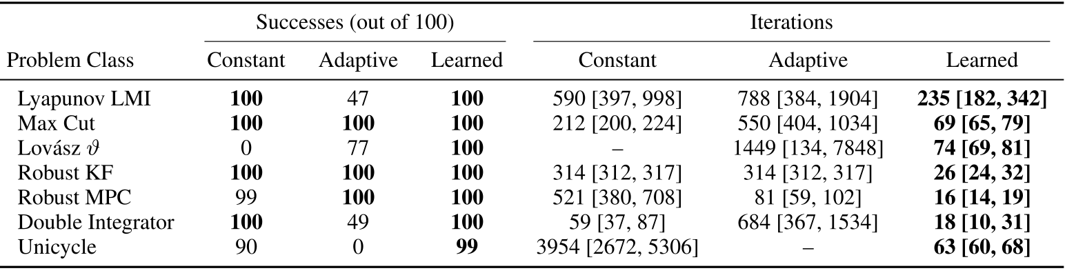
Unicycle subproblems need a median 63 learned iterations versus 3,954 for tuned constant COSMO, about 63× fewer. That inner-solve ratio differs from the full nonlinear scenario result. On the twelve scenarios solved by both learned COSMO and Clarabel, median total times are 27.9 versus 76.7 seconds, and the learned solver is faster on each; unsuccessful scenarios are excluded from that paired timing subset.
3.2 Benchmark Conic Optimization Problems
The suite includes Lyapunov, max-cut and Lovász SDPs, robust estimation/control SOCPs, and two covariance-steering families. Each main arm has 100 held-out instances, absolute residual tolerance 10⁻³ and a 10,000-iteration/60-second budget.
Learned median iterations are 235, 69, 74, 26, 16, 18 and 63 in Table 1 order, with 100 successes except 99 on unicycle. Thus it improves the tested medians but is not failure-free. Constant/adaptive success varies markedly: Lovász gives 0/77 and unicycle 90/0. Learned robust-KF iteration spread is wider despite a much lower median. The reported 1.3 GB, 29-second-per-epoch unicycle training result concerns the matrix-free implementation on this workload.
Original selectable table
| Successes (out of 100) | Iterations | |||||
|---|---|---|---|---|---|---|
| Problem Class | Constant | Adaptive | Learned | Constant | Adaptive | Learned |
| Lyapunov LMI | 100 | 47 | 100 | 590 [397, 998] | 788 [384, 1904] | 235 [182, 342] |
| Max Cut | 100 | 100 | 100 | 212 [200, 224] | 550 [404, 1034] | 69 [65, 79] |
| Lovász | 0 | 77 | 100 | – | 1449 [134, 7848] | 74 [69, 81] |
| Robust KF | 100 | 100 | 100 | 314 [312, 317] | 314 [312, 317] | 26 [24, 32] |
| Robust MPC | 99 | 100 | 100 | 521 [380, 708] | 81 [59, 102] | 16 [14, 19] |
| Double Integrator | 100 | 49 | 100 | 59 [37, 87] | 684 [367, 1534] | 18 [10, 31] |
| Unicycle | 90 | 0 | 99 | 3954 [2672, 5306] | – | 63 [60, 68] |
3.3 Batched GPU Throughput
Block-diagonal batching shares one GPU solver run across independent instances. At batch 64, max-cut takes 0.372 seconds versus sequential COSMO.jl’s 3.02; Lovász takes 5.14 versus 72.3, approximately 8.1× and 14.1× throughput gains.
These compare a batched GPU implementation against sequential CPU packages, not identical hardware or a parallel CPU baseline. Ten batches are measured per size. Faster single-instance iteration counts alone do not explain the full throughput advantage.

Original selectable table
| Max Cut | Lovász | |||
|---|---|---|---|---|
| Method | ||||
| Learned | 0.248 [0.232, 0.264] | 0.372 [0.361, 0.397] | 1.53 [1.21, 2.12] | 5.14 [3.65, 8.61] |
| COSMO.jl | 0.721 [0.625, 0.757] | 3.02 [2.74, 3.28] | 9.63 [9.13, 10.3] | 72.3 [39.8, 98.2] |
| Clarabel | 3.70 [3.60, 3.76] | 14.9 [14.7, 17.4] | 68.6 [68.4, 69.0] | 276 [275, 277] |
3.4 Out-of-Distribution Generalization
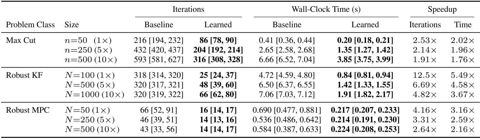
Policies trained at one size are tested on twenty fresh instances at each larger size. Ten times more graph nodes increases max-cut variables from 1,275 to 125,250; longer SOCP horizons instead add similarly sized cone blocks.
All arms finish in this experiment. At 10×, time speedups are 1.76× max-cut, 3.67× robust KF and 2.16× robust MPC, so the abstract’s 2–5× shorthand is not exact for every row. Max-cut transfer also uses a factor-five penalty-adoption gate after updating every iteration caused divergence. Weights are unchanged, but execution policy is modified; the full qualification is retained in Appendix J.
Original selectable table
| Iterations | Wall-Clock Time (s) | Speedup | |||||
|---|---|---|---|---|---|---|---|
| Problem Class | Size | Baseline | Learned | Baseline | Learned | Iterations | Time |
| Max Cut | () | 216 [194, 232] | 86 [78, 90] | 0.41 [0.36, 0.44] | 0.20 [0.18, 0.21] | ||
| () | 432 [420, 437] | 204 [192, 214] | 2.65 [2.58, 2.68] | 1.35 [1.27, 1.42] | |||
| () | 593 [581, 627] | 316 [308, 328] | 6.66 [6.52, 7.04] | 3.85 [3.75, 3.99] | |||
| Robust KF | () | 318 [314, 320] | 25 [24, 37] | 4.72 [4.59, 4.80] | 0.84 [0.81, 0.94] | ||
| () | 320 [317, 321] | 48 [39, 60] | 6.50 [6.37, 6.55] | 1.42 [1.33, 1.55] | |||
| () | 320 [319, 322] | 66 [62, 80] | 7.06 [7.03, 7.12] | 1.91 [1.82, 2.17] | |||
| Robust MPC | () | 66 [52, 91] | 16 [14, 17] | 0.690 [0.477, 0.881] | 0.217 [0.207, 0.233] | ||
| () | 46 [39, 51] | 14 [13, 16] | 0.536 [0.486, 0.642] | 0.214 [0.191, 0.230] | |||
| () | 43 [33, 56] | 14 [14, 17] | 0.584 [0.387, 0.633] | 0.224 [0.208, 0.253] | |||
4 Limitations
Dense eigendecomposition of a p×p PSD block still costs O(p³); the stable backward rule does not remove this limit. Benefits depend on sparse problem structure, moderate residual tolerance and amortizing per-family training across many solves. Tight-accuracy superiority over interior-point methods is not claimed.
The study does not establish universal convergence of learned schedules or reliable real-time hardware deployment. Other ADMM solvers, mixed-size training and physical testing remain future work.
Acknowledgments
The authors acknowledge reviewer feedback on the analysis and presentation.
Appendix A Related Work
Learning to optimize and deep unfolding.
LISTA and later algorithm-unrolling work motivate learning within known iterative structure. This provides interpretability and budgeted training, but retaining the update form is not by itself a proof that every learned parameter trajectory inherits the original solver’s guarantees.
Learned QP and conic solvers.
Learned fixed-point warm starts predict initialization; linearized Douglas–Rachford unfolding avoids full inner solves; learned parameter policies adjust the trajectory using current residuals. This paper keeps the full conic update and makes its backward pass tractable.
Differentiable optimization layers.
OptNet and differentiable convex layers differentiate an optimal solution with respect to problem data. A fully converged solution does not depend on algorithmic penalties, so that route does not train their convergence speed. Unrolling exposes finite-iteration behavior; the internal solve still benefits from implicit differentiation.
First-order conic solvers.
SCS, OSQP and COSMO use operator splitting. Indirect solves suit sparse GPU computation, while slow high-accuracy convergence motivates the study’s moderate tolerance. Clarabel supplies a separate interior-point comparison.
Differentiating through eigendecompositions.
Matrix-backpropagation analysis and alternative eigendecomposition gradients explain the repeated-eigenvalue problem. The paper adapts a known spectral derivative to PSD projections inside learned optimization; it does not introduce the general matrix-function theorem.
Appendix B Details on Linear-System Solve Backward Pass Experiment (Figure 2)
The backward benchmark uses n=1,000–50,000, m=n/2, diagonal P and A with 1% density, with 100 random instances per size. Baselines explicitly form dense saddle-point or reduced-system intermediates; open dashed markers extrapolate configurations exceeding the 24 GB limit.
The reported matrix-free peak stays below 300 MB at n=50,000. However, fixed 1% density gives nnz(A)=0.005n²: storage proportional to sparse nonzeros is still quadratic in n for this generator. The advantage is avoiding much larger dense intermediates, not a general linear-in-n bound under fixed density. Dense baselines also do not represent every possible optimized sparse factorization implementation.
Appendix C Details on PSD Projection Backward Pass Experiments (Figures 3 and 4)
One test follows a 100-iteration covariance-steering trajectory with collapsing eigenvalue gaps; ordinary autograd eventually produces NaNs, regularization biases gradients and Newton–Schulz has spikes, while DK remains near the observed error floor.
A controlled test uses forty-dimensional symmetric matrices with clusters centered at ±δ/2 and within-cluster spread 10⁻³δ, over δ=1 to 10⁻¹⁰. Timing sweeps dimensions 10–320 over 100 samples. Newton–Schulz can have lower finite-difference error than DK but is roughly an order of magnitude slower. These two experiments address different regimes; ordinary autograd remains finite in the controlled one.
Equation 14
| (14) |
Appendix D Training Details
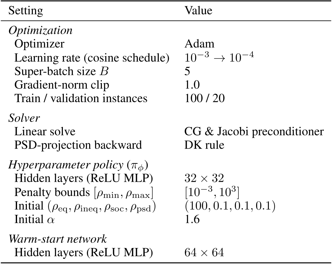
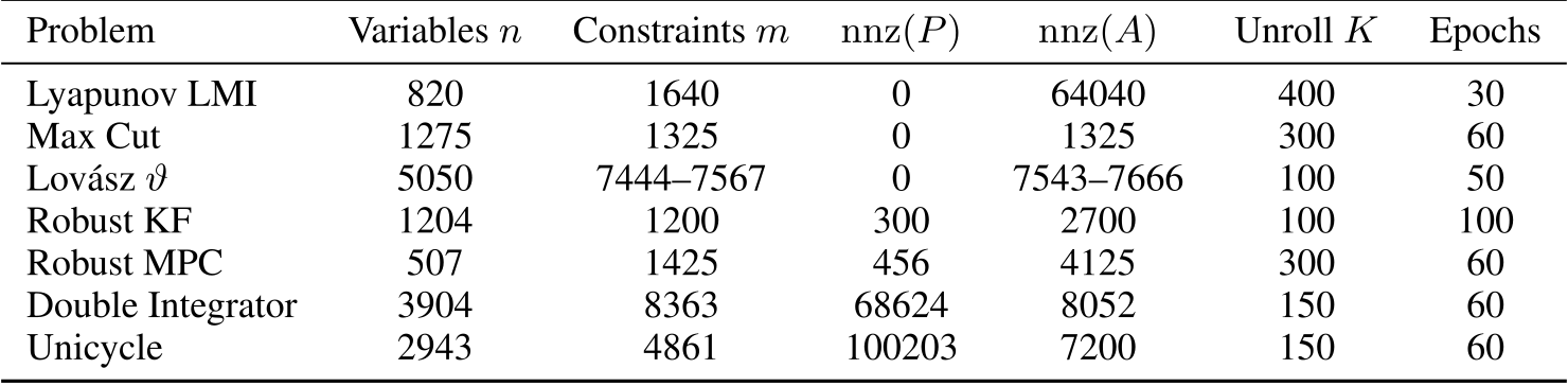
Each family trains policy and warm-start modules in double precision using Adam, cosine learning rate 10⁻³→10⁻⁴, batch five and gradient clipping 1.0. The lowest validation-loss checkpoint is selected; each model takes under ten GPU hours. Tables 4–5 retain all sizes, 30–100 epochs and 100–400-step unroll horizons.
Jacobi-preconditioned CG uses relative tolerance 10⁻⁸ during training and absolute 10⁻⁴ at inference; the authors report the same ordering across tested inference tolerances. The nonlearned comparisons start from zero. Sparse P storage can be substantial, as the covariance-steering rows show, so total memory is not described by A alone.
Original selectable table
| Setting | Value |
|---|---|
| Optimization | |
| Optimizer | Adam |
| Learning rate (cosine schedule) | |
| Super-batch size | 5 |
| Gradient-norm clip | 1.0 |
| Train / validation instances | 100 / 20 |
| Solver | |
| Linear solve | CG & Jacobi preconditioner |
| PSD-projection backward | DK rule |
| Hyperparameter policy () | |
| Hidden layers (ReLU MLP) | |
| Penalty bounds | |
| Initial | |
| Initial | 1.6 |
| Warm-start network | |
| Hidden layers (ReLU MLP) | |
Original selectable table
| Problem | Variables | Constraints | Unroll | Epochs | ||
|---|---|---|---|---|---|---|
| Lyapunov LMI | 820 | 1640 | 0 | 64040 | 400 | 30 |
| Max Cut | 1275 | 1325 | 0 | 1325 | 300 | 60 |
| Lovász | 5050 | 7444–7567 | 0 | 7543–7666 | 100 | 50 |
| Robust KF | 1204 | 1200 | 300 | 2700 | 100 | 100 |
| Robust MPC | 507 | 1425 | 456 | 4125 | 300 | 60 |
| Double Integrator | 3904 | 8363 | 68624 | 8052 | 150 | 60 |
| Unicycle | 2943 | 4861 | 100203 | 7200 | 150 | 60 |
Appendix E Policy Parameterization
Hyperparameter policy.
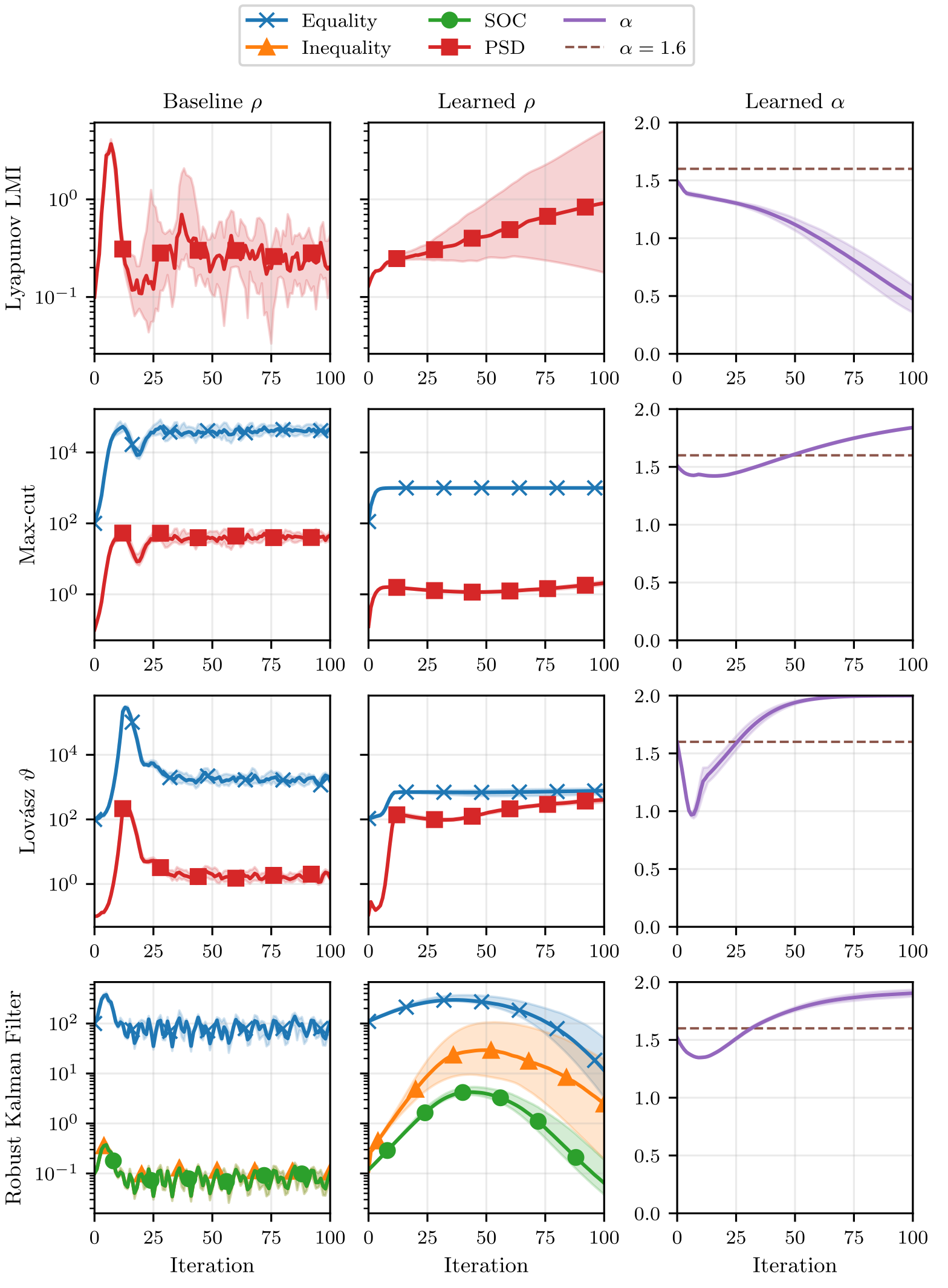
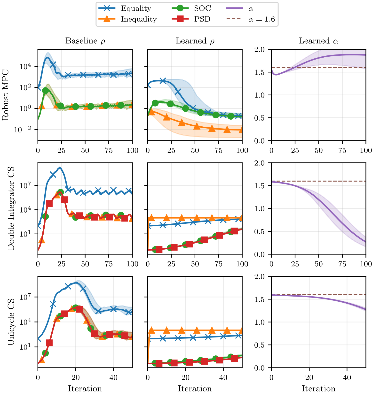
Shared residual-conditioned MLPs update logits recurrently. Squashed outputs keep penalties between 10⁻³ and 10³ and relaxation between zero and two. Features combine normalized global KKT residuals with local slack changes and projection mismatch; all exact feature formulas remain available.
Zero-initialized output layers begin at constant COSMO parameters, with learnable initial logits. Averaging within each nonseparable cone supplies one scalar penalty for its ordinary Euclidean projection. Per-row penalties remain for zero/nonnegative cones. The bounds and initialization improve training behavior but do not supply a general convergence theorem.
Equations
Warm-start network.
Two shared 64×64 MLPs predict variable and constraint initialization from local cost/matrix statistics, cone type and pooled scale/size features. Zero output initialization recovers the baseline zero iterate and allows the same weights to accept different problem sizes.
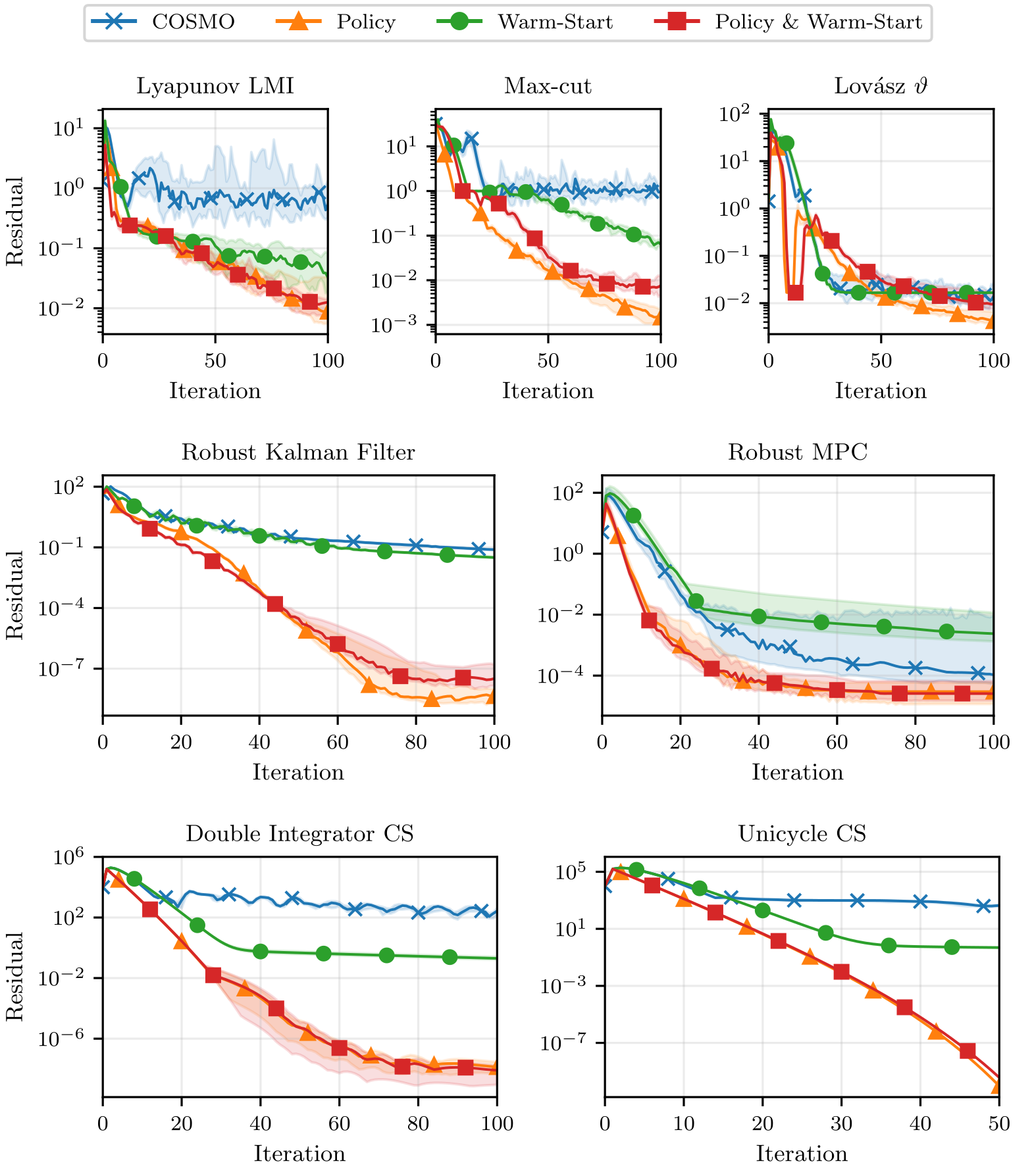
Figure 5 attributes most gains to the adaptive policy: warm starts can hurt robust MPC, and joint training offers little extra over the policy alone. The benchmark descriptions nevertheless specify policy plus warm-start modules for the learned arm. Figures 6 and its continuation preserve every problem-family penalty/relaxation plot; cone-specific penalties differ from a scalar residual-balancing rule.
Appendix F Conic Optimization Problems
Unless stated otherwise, datasets use 100 training, twenty validation and 100 independently seeded test problems per family. The complete conic formulations and generator settings follow; generated distributions and filtering are part of the benchmark scope.
F.1 Covariance Steering
Stacked linear dynamics and strictly causal disturbance feedback U=KW+V separate mean control from covariance shaping. Covariance upper bounds become Schur-complement LMIs, retaining a convex formulation rather than a nonconvex low-rank factorization.
For nonlinear dynamics, SCP linearizes around a reference, adds penalized virtual control to mean dynamics and accepts steps using a trust-region ratio. Virtual control relaxes those dynamics; it does not by itself guarantee feasibility of every covariance, boundary or trust-region constraint.
Double-integrator instances use horizon thirty, step 0.5, random target position and the stated diagonal process-noise covariance. Unicycle uses horizon thirty, step 0.1, randomized heading/targets/covariance bounds and virtual-control weight 10⁴. The paper’s exact covariance choices are preserved rather than silently replacing them with a different continuous-noise discretization.
For unicycle training, twelve scenarios generate ten Clarabel subproblems each: ten scenarios supply 100 training subproblems and two supply twenty validation subproblems. Ten independent scenarios supply the standalone test set; twenty further scenarios evaluate full SCP. Correlated subproblems within one scenario are not independent original planning problems.
Equations
F.2 Lyapunov Linear Matrix Inequality
A forty-state stable linear system supplies a minimum-trace Lyapunov SDP with AᵀP+PA≼−I and P≽I. Two equally likely generators vary nonnormal upper-triangular dynamics or damped oscillator blocks under orthogonal transforms. Cases with spectral abscissa not below −0.05 are resampled. The trace objective normalizes the selected certificate; the notes do not assume strict convexity or uniqueness from a linear objective alone.
Equations
F.3 Max Cut
The standard max-cut SDP maximizes one quarter of the Laplacian inner product subject to unit diagonal and PSD X, following Goemans–Williamson. Training graphs have fifty nodes and edge probability 0.5. Solver speed is measured on the relaxation, not on a rounded discrete cut or its approximation quality.
Equation
F.4 Lovász ϑ
The Lovász theta SDP maximizes the all-ones inner product with trace one, zero edge entries and PSD X. Erdős–Rényi training graphs have one hundred nodes and edge probability 0.5. This is a different graph relaxation from max-cut despite shared PSD machinery.
Equation
F.5 Robust Kalman Filter
The robust estimation SOCP fits a dragged double-integrator trajectory using quadratic process-noise cost and Huber observation residuals, adapted from the CVXPY example. Horizon is one hundred, step 0.1, drag 0.05 and both Huber parameters are two. Observations use an 80% unit-noise/20% standard-deviation-twenty mixture. It is a batch trajectory-estimation benchmark, not a measured online filter on a physical sensor.
Equations
F.6 Robust Model Predictive Control
The MPC benchmark uses nominal linear dynamics, covariance-based half-space tightening, control-norm epigraph costs and a penalized terminal distance. It models three spring-coupled masses with six states/three inputs, horizon fifty and step 0.2. State boxes are position ±5 and velocity ±1; input bounds are ±0.5. Disturbance scale is 0.01 and κ=2.
The description calls the formulation robust to every bounded ellipsoidal disturbance. Its covariance recursion and root-sum-square tightening do not generally give that worst-case guarantee over independently bounded disturbances; such reachable-set support radii accumulate as a sum. Appendix H instead samples unbounded Gaussian disturbances. The formulas and observed outcomes remain, without promoting the label to a universal safety certificate.
About 10% of candidate initial states/penalties are rejected if Clarabel finds infeasibility or an optimal dual norm above 150. This filters the evaluation distribution. The terminal target is softly penalized through an epigraph, not enforced as a hard equality.
Equations
Appendix G Additional Benchmarks
CPU COSMO.jl and Clarabel use eight BLAS threads, warm-up and 10⁻³ tolerances; chordal decomposition is disabled. COSMO.jl otherwise retains scaling, adaptive penalties and Anderson acceleration, while Clarabel retains presolve/equilibration.
Learned GPU COSMO is fastest for Lovász and both covariance-steering classes. COSMO.jl is faster on Lyapunov and max-cut, and Clarabel is much faster on the small robust-KF/MPC SOCPs: learned/Clarabel medians are 0.884/0.00208 seconds and 0.216/0.00193 seconds. These results qualify any claim of universal wall-clock superiority, and disabling decomposition limits the comparison with fully configured sparse SDP packages.

Original selectable table
| Problem Class | Constant | Adaptive | Learned | COSMO.jl | Clarabel |
|---|---|---|---|---|---|
| Lyapunov LMI | 1.58 [1.04, 3.11] | 2.42 [1.26, 5.39] | 1.09 [0.761, 1.52] | 0.462 [0.398, 0.590] | 0.593 [0.519, 0.721] |
| Max Cut | 0.396 [0.376, 0.421] | 1.08 [0.788, 2.01] | 0.159 [0.149, 0.179] | 0.0411 [0.0382, 0.0492] | 0.229 [0.205, 0.239] |
| Lovász | – | 1.01 [0.547, 12.2] | 0.359 [0.333, 0.391] | 0.599 [0.523, 0.773] | 4.27 [4.23, 4.31] |
| Robust KF | 4.62 [4.50, 4.75] | 4.64 [4.52, 4.79] | 0.884 [0.831, 0.966] | 0.0169 [0.0167, 0.0171] | 0.00208 [0.00205, 0.00213] |
| Robust MPC | 1.02 [0.842, 1.35] | 0.821 [0.633, 1.02] | 0.216 [0.196, 0.248] | 0.0137 [0.0134, 0.0154] | 0.00193 [0.00173, 0.00195] |
| Double Integrator | 0.971 [0.531, 1.57] | 4.81 [3.03, 9.20] | 0.633 [0.428, 0.734] | 2.73 [2.53, 2.95] | 14.1 [12.8, 14.5] |
| Unicycle | 31.4 [21.3, 40.9] | – | 0.911 [0.808, 0.992] | 1.48 [1.22, 2.16] | 3.82 [3.53, 3.98] |
Appendix H Control Performance and Failure Modes
This appendix checks control outcomes beyond solver residuals. Results are simulated and conditional on the returned solutions; both incomplete inner solves and failures of the outer planning loop matter.
Failure modes for nonlinear covariance steering.
Each nonlinear scenario has twenty SCP steps and up to twenty seconds per subproblem. Learned COSMO fails four scenarios: two finish near residual 0.0033, and two stall at 0.29/0.99 despite later inner solves converging. Clarabel fails eight: five repeatedly return no solution, three stall despite solved subproblems.
Clarabel fails on all four scenarios failed by the learned solver. Conversely, learned COSMO succeeds on three scenarios containing timed-out inner solves. Inner residual convergence and full nonlinear planning success are therefore related but not interchangeable.
Monte Carlo validation of the covariance bounds.
For each successfully solved unicycle scenario, 2,000 shared-noise rollouts test the affine disturbance-feedback policy on the nonlinear Euler dynamics. Empirical terminal covariance stays below its target, with largest-eigenvalue margins from −0.05 to −0.00051; terminal mean error is at most 0.0071. Median empirical/predicted cost ratios are 1.0006 learned and 1.0003 Clarabel.
This validates the reported successful scenarios under sampled disturbances. It does not cover failed scenarios or prove a population covariance bound from finite Monte Carlo samples.
Closed-loop robust MPC.
Ten fifty-step closed-loop MPC episodes use Gaussian process noise. On nine episodes, all methods converge at every step without state violations; learned cost nearly matches Clarabel. Learned median time is 0.29 seconds versus adaptive COSMO 2.10 and CPU Clarabel 0.035, so even the learned median exceeds the model’s 0.2-second sampling interval.
On the remaining episode all methods fail early. Learned COSMO and Clarabel apply zero after nonfinite/no solutions and violate the state box on four steps by up to 0.42; adaptive COSMO applies inexact iterates and violates three steps by up to 0.08. A returned approximate iterate or zero-control fallback is not certified safe, and the reported failures remain visible.
Appendix I Details on Batched Solve Experiment (Table 2)
Instances.
Fresh, nonrepeated batches of 8/16/32/64 graphs use the same distribution as training-size test data. Ten batches per size share instances across solvers. Relative throughput grows with batch size; Table 2 displays the sixteen- and sixty-four-instance cases.
Learned solver.
The learned arm batches sparse operators, cone projections and policy evaluation. It stops only once every instance meets tolerance; already converged instances keep iterating, so slower members control batch duration. Median Lovász batch iterations rise from 154 to 434 as batch size grows from eight to sixty-four. All tested batches finish within 10,000 iterations/60 seconds.
Timing.
GPU timing includes batch assembly and solver construction, reported as 1–3% of total, after warm-up absorbs initialization. CPU totals sum each package’s native sequential solve/setup times. CUDA synchronization is explicit; this benchmark concerns throughput under those implementations, not a hardware-neutral algorithmic ratio.
Appendix J Details on Out-of-Distribution Experiment (Table 3)
Instances.
Scaling graph nodes increases the max-cut PSD block from 50×50 to 500×500, whereas scaling KF/MPC horizons adds fixed-size SOC blocks. Twenty instances per size use unchanged generator parameters; these are new samples, so the 1× statistics differ from Table 1.
Arms.
Row-wise shared features let trained policy/warm-start weights accept new sizes. SOCP penalties update every iteration. Max-cut instead adopts a predicted penalty only after a factor-five change because unrestricted updates diverged under shifted residual scales.
The baseline is the adaptive residual-balancing arm with the same gate and zero initialization; tuned constants are omitted because they are training-size-specific. Thus “best-tuned baseline” in the table caption should be read in light of this narrower protocol. No retraining does not mean every inference setting is unchanged.
Protocol.
Every size uses residual tolerance 10⁻³ and a 10,000-iteration/600-second cap; neither arm fails. Speedups are medians of paired instance ratios, which need not equal ratios of the displayed median times. Robust-KF iteration growth reflects shifted difficulty, robust-MPC baseline iterations decrease with horizon, and max-cut gets harder for both arms.