Overview
This edition covers the complete 29-page v2 dated 13 October 2026. It retains all method details, repeated evaluations, sensitivity studies, runtime measurements and failure analysis. The learned policy is unchanged at deployment; robot-specific geometry enters the sampling procedure.
At a glance
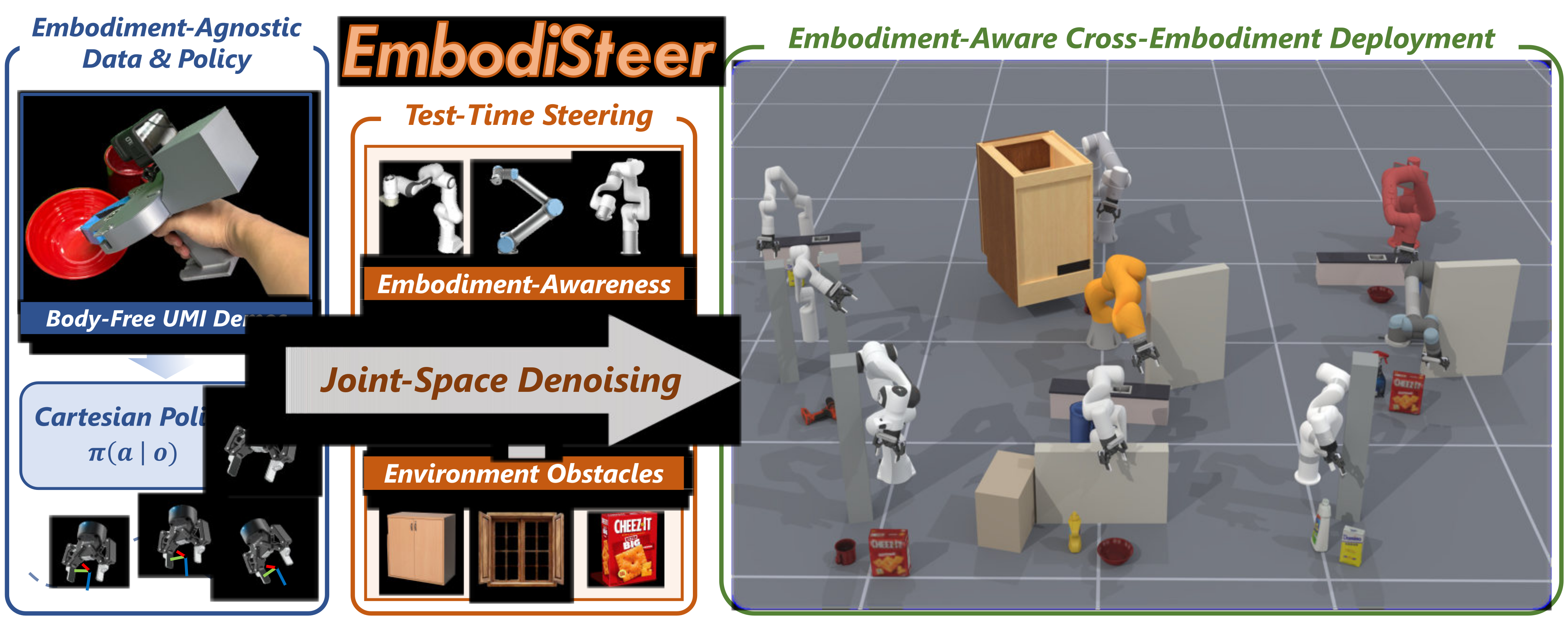
EmbodiSteer maintains a joint trajectory while querying a frozen Cartesian diffusion policy through forward kinematics. Damped Jacobian updates follow the policy’s denoising residual, then a local quadratic program moves the whole arm away from obstacles while penalizing end-effector deviation.
Across nine simulated arms, the main evaluation improves success from 35.7% to 64.2% and reduces collision occurrence from 57.6% to 11.5%. Across two physical arms and three tasks, success rises from 25/60 to 47/60 and collisions fall from 58/60 to 4/60. These are empirical results with modeled obstacles, not a formal safety guarantee.
1 Introduction
Cartesian end-effector actions make heterogeneous robot and UMI handheld-gripper demonstrations share one action representation, but do not describe the deployed arm’s links or feasible joint configurations. Reproducing a gripper path can therefore cause elbow or forearm collisions.
The paper separates this execution problem from learning a new embodiment-specific policy. It preserves a pretrained Diffusion Policy and introduces the target kinematics and whole-body constraints during sampling, requiring no target-arm demonstrations or finetuning.
2 Related Work
Cross-embodiment approaches align action representations through decoders, reusable skills or embodiment conditioning; XMoP instead learns a transferable whole-body motion planner. EmbodiSteer adds body awareness to an existing Cartesian manipulation policy at deployment.
Inference guidance can bias, filter or optimize diffusion samples. JM2D combines learned planners and model-based constraints through joint sampling, while EADP emphasizes controller tracking for aerial manipulation. This work targets arm-body obstacle avoidance while retaining the manipulation policy’s task motion.
Safety filters, control barrier functions, collision-guided diffusion and dedicated whole-body planning policies provide related mechanisms. EmbodiSteer uses a local CBF-inspired correction, without learning a new collision-aware trajectory representation or claiming a global certificate.
3 Preliminaries: Cartesian Diffusion Policy
The base model learns to predict Gaussian noise added to demonstration action chunks, then samples by reverse denoising. Each action contains relative translation, a continuous six-dimensional rotation representation and a gripper command; the main equations omit the gripper for brevity.
Poses are relative to the chunk-start end effector, so the action semantics are independent of arm joint count and ordering. Equation 1 presents a DDPM update; implementation uses a 16-step DDIM scheduler.
Equation 1
| (1) |
Equations
4 Method
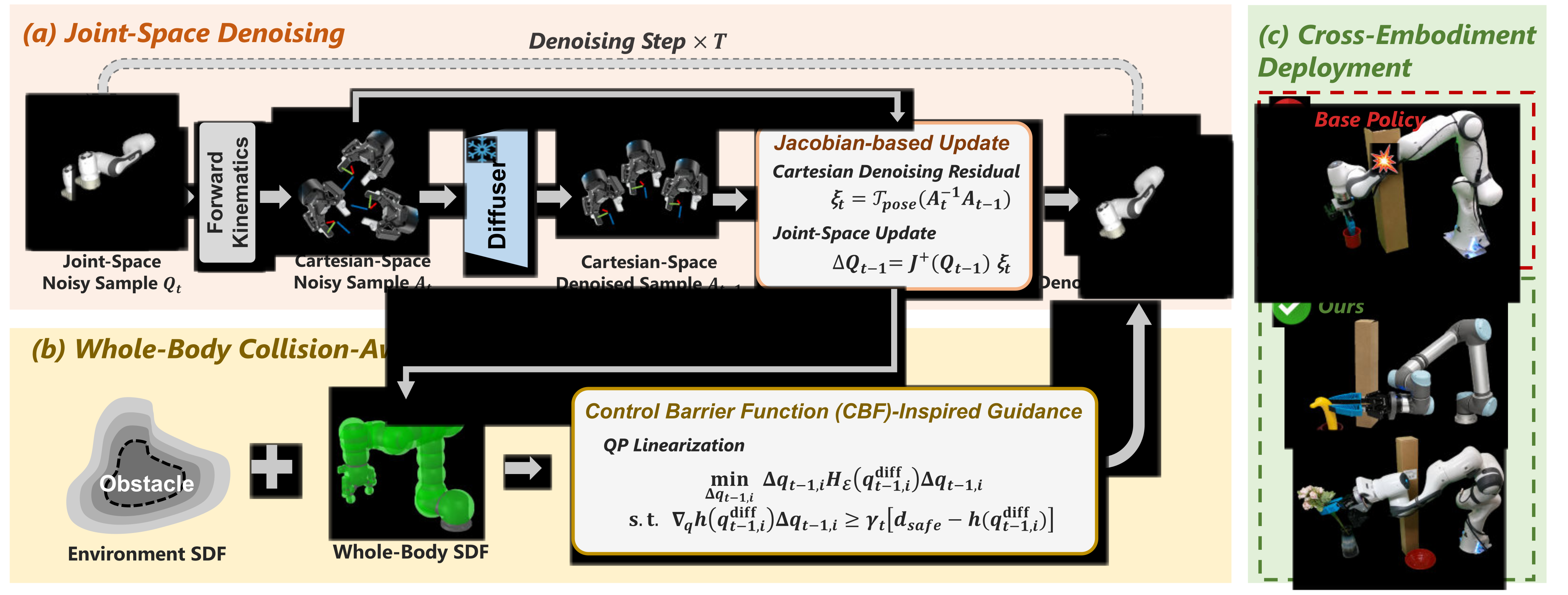
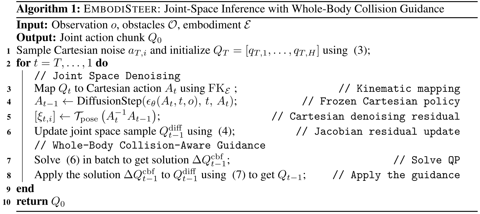
Inference alternates two operations: use the frozen Cartesian denoiser to propose task progress, then correct the corresponding joint states using target-robot geometry. Algorithm 1 retains the complete procedure.
4.1 Problem Formulation
The target robot has a joint vector at each action-horizon step. A whole-body signed-distance function measures clearance from known obstacles, and the desired condition is clearance at least a positive margin at every sampled state.
This waypoint condition does not itself certify motion between states. The implemented distance is a smooth approximation over collision spheres, and both the nonlinear geometry and joint correction are subsequently approximated.
Equation 2
| (2) |
Selectable original pseudocode
4.2 Joint-Space Denoising with Pretrained Cartesian Diffusion Policy
Repeated inverse-kinematics solves within diffusion are expensive. Instead, map each local six-dimensional pose residual through a damped Jacobian pseudoinverse. Damping limits amplification near singularities; clipping bounds each per-joint update.
Initialize around the current configuration by projecting Cartesian Gaussian noise into joint perturbations, then scaling and clipping. This is a local kinematic construction, rather than an exact preservation proof for the original Cartesian sampling distribution.
Equations 3
| (3) |
Joint-Space Denoising Update.
Forward kinematics converts the current noisy joint chunk back into the denoiser’s relative Cartesian representation. The frozen network proposes the next Cartesian chunk. Its relative pose residual becomes a translation/rotation twist, which the damped Jacobian maps into a clipped joint increment.
Equations 4
| (4) |
4.3 CBF-Inspired Whole-Body Collision-Aware Guidance
Plain collision-cost gradients can move an elbow away from an obstacle while displacing the gripper from a precise grasp or contact. The guidance objective therefore explicitly penalizes task-space motion, rather than treating all joint-space escape directions equally.
Equation
CBF-Inspired Guidance Formulation.
For each horizon state independently, the nonlinear objective balances weighted end-effector deviation and joint deviation subject to a clearance margin. Position and rotation receive separate weights; joint regularization discourages unnecessarily large corrections.
Equation 5
| (5) |
QP Linearization for Efficient Update.
Linearizing forward kinematics and clearance yields a positive regularized quadratic cost with one linear inequality. Its matrix combines the Jacobian task metric and an identity regularizer; a scheduled strength determines how aggressively the margin deficit is corrected.
The single-constraint problem admits a closed-form solution. The resulting joint increment is clipped again before use. Linearization, smoothing, the numerical stabilizer and clipping mean this is practical collision guidance, not certified feasibility of the original nonlinear constraint.
Equations 6–7
| (6) |
| (7) |
Equation
5 Results
The evaluation separates transfer without obstacles, obstacle-aware execution in simulation, and physical deployment. Success, reward and collision occurrence measure different outcomes and should be read together.
5.1 Simulation Results
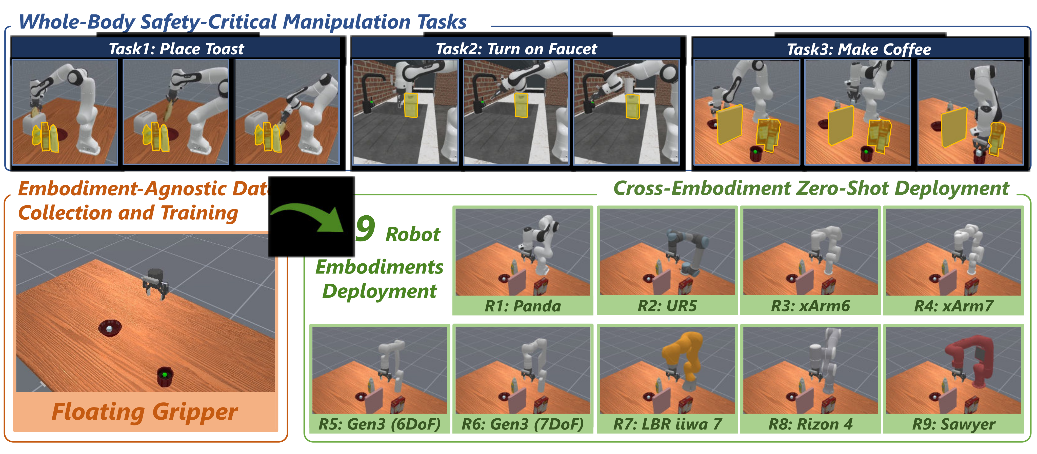
Each of three ManiSkill tasks uses 200 obstacle-free floating-gripper demonstrations. The same wrist camera and gripper mount are retained across nine arms; the learned policy receives wrist RGB and end-effector state. Obstacles appear only at deployment in the main benchmark.
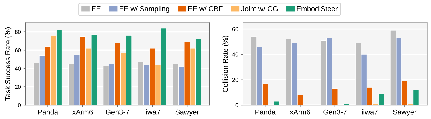
Without obstacles, Cartesian and unguided joint sampling average 90.0% and 90.7% success. With obstacles, EmbodiSteer reaches 64.2% success and 11.5% collisions versus 57.0% and 17.9% for a one-shot post-hoc CBF correction. Candidate sampling offers only a modest gain, while unregularized collision gradients can substantially hurt precise tasks.
Three evaluation seeds using the same trained policies give 63.3±1.4% success and 11.7±.8% collisions for EmbodiSteer, versus 36.0±.2% and 56.8±.9% for Cartesian execution. These deviations quantify evaluation-seed variation, not independent policy training runs.
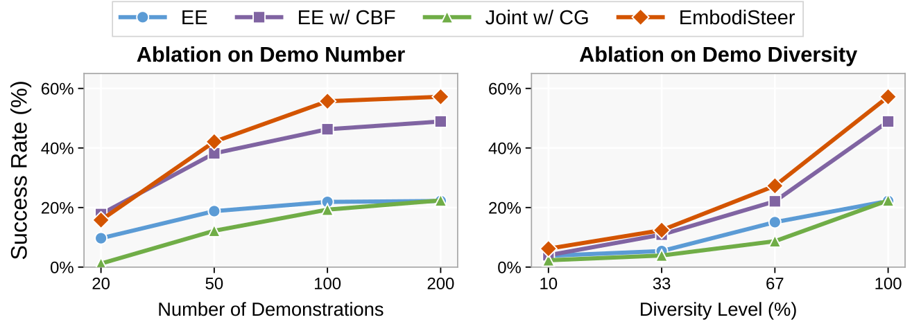
A JM2D-style adaptation takes 8.65 seconds per chunk with 16 proposals and 16 denoising steps, versus .254 seconds for EmbodiSteer on the matched RTX 4090 setup. Only computational feasibility is compared; no full task-performance result is reported for that adaptation. Increasing demonstration quantity or waypoint diversity improves performance under guidance-induced perturbations.
| Obstacles | Method | PlaceToast | TurnOnFaucet | MakeCoffee | Average | ||||||||
| TSR | RWD | COR | TSR | RWD | COR | TSR | RWD | COR | TSR | RWD | COR | ||
| w/o Obs. | EE | 96.8 | .980 | – | 83.6 | .937 | – | 89.7 | .932 | – | 90.0 | .950 | – |
| Joint | 94.4 | .965 | – | 87.9 | .957 | – | 89.7 | .929 | – | 90.7 | .950 | – | |
| w/ Obs. | EE | 43.4 | .634 | 52.6 | 41.6 | .752 | 61.8 | 22.2 | .456 | 58.3 | 35.7 | .614 | 57.6 |
| EE w/ Sampling | 47.1 | .661 | 51.3 | 43.9 | .767 | 53.2 | 24.1 | .478 | 60.0 | 38.4 | .635 | 54.8 | |
| EE w/ CBF | 65.8 | .764 | 15.3 | 56.3 | .797 | 29.9 | 48.9 | .606 | 8.6 | 57.0 | .722 | 17.9 | |
| Joint w/ CG | 57.7 | .687 | 0.2 | 10.3 | .403 | 59.6 | 22.4 | .424 | 40.6 | 30.1 | .505 | 33.5 | |
| EmbodiSteer | 74.8 | .829 | 4.6 | 60.6 | .833 | 27.1 | 57.2 | .670 | 2.8 | 64.2 | .777 | 11.5 | |
| Method | TSR (%) | RWD | COR (%) |
| EE | |||
| EE w/ Sampling | |||
| EE w/ CBF | |||
| Joint w/ CG | |||
| EmbodiSteer |
5.2 Real-World Experiments
UR5 and Franka Panda share one UMI-trained Cartesian checkpoint per task, with 200 obstacle-free demonstrations and no robot-specific finetuning. Each robot-task pair has ten no-obstacle trials and ten obstacle trials.
The base policy succeeds 49/60 times without obstacles. Under obstacles, success is 25/60 with 58/60 collisions; guidance yields 47/60 successes and 4/60 collisions. The changes are +36.7 and −90.0 percentage points. Movable obstacles permit task completion after contact, so success and collision are annotated independently.
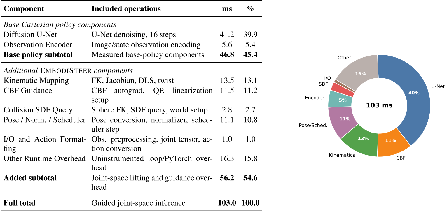
A separate runtime breakdown measures 103 ms for one guided call on an RTX 4070 Ti SUPER, approximately 9.7 calls per second. This measurement differs from the synchronized RTX 4090 comparison and should not be directly combined with it.
6 Limitations & Conclusion
Guidance is local: it becomes active near the modeled clearance margin and cannot choose globally collision-free routes far in advance. Nonlinear geometry, clipped updates and strong corrections can leave collisions unresolved or move observations outside the policy’s training distribution.
The contribution is a training-free bridge between embodiment-agnostic action learning and embodiment-specific execution. Broader demonstrations help, but known geometry and local linearization remain material restrictions.
Acknowledgments
The authors acknowledge discussions, hardware and experimental assistance, and reviewer feedback.
Appendix A Method Details
The appendix makes the action representation, signed-distance convention and one-constraint quadratic-program solution explicit. All original numbered expressions and substantive inline definitions are retained.
A.1 Cartesian Action Conversion and Pose-Twist Mapping
The chunk-start pose converts relative translation and six-dimensional rotation into world-frame end-effector poses. The shorthand inverse action product denotes the relative rigid transform, not inversion of a raw nine-dimensional vector.
The pose-twist operator concatenates relative translation and the rotation-vector logarithm. Initialization uses the current chunk-start joints; damped Jacobian updates and per-joint clipping control the error of this local approximation.
Equations 8–10
| (8) |
| (9) |
| (10) |
A.2 Whole-Body SDF Representation
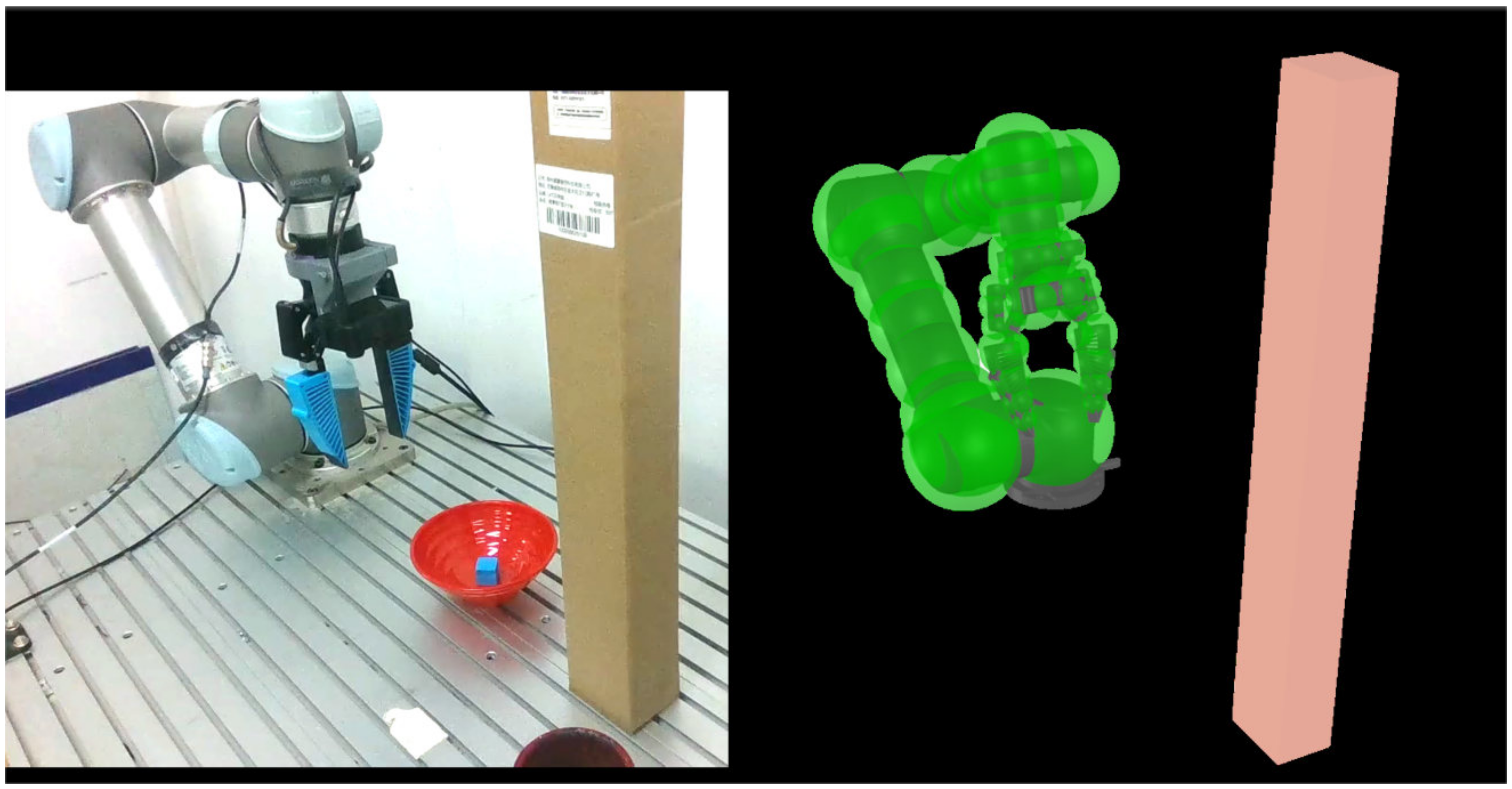
cuRobo approximates links with collision spheres and queries known cuboid obstacles. Its signed distance is positive for penetration, opposite the main paper’s positive-clearance convention. Exact worst clearance is the negative maximum sphere distance.
Guidance instead uses the negative normalized log-sum-exp of the four largest sphere distances, with temperature 20. This smooth maximum is at most the true maximum, so the resulting clearance can be optimistic; the source describes the bias without bounding its safety effect. Unknown-obstacle perception is outside scope.
Equations 11–13
| (11) |
| (12) |
| (13) |
A.3 CBF-Inspired QP Details
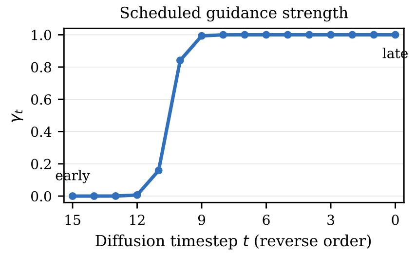
The regularized Jacobian metric gives a one-constraint QP. The schedule follows constraint-aware diffusion guidance: a sigmoid with slope 50 and transition .7 is weak at early noisy steps and approaches the base strength later. Already-safe states receive zero correction through a nonnegative constraint deficit.
The KKT derivation yields a correction along the inverse-metric clearance gradient, scaled by the deficit divided by its quadratic norm. A small denominator stabilizer and subsequent clipping modify the ideal solution. Only arm joints are corrected; gripper commands remain unchanged.
Equations 14–16
| (14) |
| (15) |
| (16) |
Equations 17–18
| (17) |
| (18) |
Appendix B Implementation Details
Implementation details specify the shared visual policy, deployment parameters, runtime accounting and all baseline procedures.
B.1 Diffusion Policy Architecture
A pretrained CLIP ViT-B/16 visual encoder is finetuned jointly with a conditional one-dimensional U-Net. Two observations condition sixteen ten-dimensional actions: three translation, six rotation and one gripper coordinate. Deployment freezes the model and uses sixteen DDIM denoising steps.
B.2 Hyperparameters
Table 3 retains all training and deployment settings. Policies train for 120 epochs with AdamW and EMA; control runs at 10 Hz. Sixteen actions are executed before replanning in simulation, six on hardware.
Default Jacobian damping is .001, projected-noise scale .1, denoising joint clip .5, QP regularization .01 and guidance clip .1. Task-dependent safety margins are .05–.10, with position/rotation weights 1/.1 and four critical collision spheres.
| Quantity | Value | Notes |
| Observation horizon | 2 | Diffusion policy input setting. |
| Action horizon | 16 | Predicted action chunk length. |
| Execution horizon | 16 in simulation, 6 in real world. | Number of actions executed before replanning. |
| Visual backbone | CLIP ViT-B/16 | vit_base_patch16_clip_224.openai loaded through timm, pretrained and finetuned. |
| U-Net channels | [256, 512, 1024] | Conditional 1D U-Net downsampling dimensions. |
| Diffusion step embedding | 128 | Timestep embedding dimension. |
| Diffusion training timesteps | 50 | Squared-cosine beta schedule and epsilon prediction. |
| Inference denoising steps | 16 | DDIM reverse diffusion steps at deployment. |
| Control frequency | 10 | Simulation and real-world control rate. |
| Training epochs | 120 | Used for both simulation and real-world policies. |
| Batch size | 128 in simulation, 64 in real world. | Training batch size for simulation and real-world checkpoints. |
| Optimizer | AdamW | Learning rate , betas , weight decay . |
| Learning-rate schedule | Cosine | 2000 warmup steps. |
| EMA | 0.9999 max decay | EMA enabled during training. |
| Image augmentation | Crop + color jitter | Random crop ratio 0.95; brightness 0.3, contrast 0.4, saturation 0.5, hue 0.08. |
| Noise initialization scale | 0.1 | Scale for Jacobian-projected noise. |
| Jacobian damping | 0.001 | Used in . |
| Joint update clip | 0.5 | Used in joint denoising update. |
| Safety margin | 0.050.10 | Task-dependent; set to 0.05, 0.07, or 0.10 by obstacle layout. |
| SDF aggregation top- | 4 | Number of critical collision spheres. |
| Smoothmax temperature | 20.0 | Temperature in (12). |
| Base constraint strength | 1.0 | Base multiplier in (16). |
| QP regularization | 0.01 | Joint-space regularization. |
| Task position weight | 1.0 | Position rows in . |
| Task rotation weight | 0.1 | Rotation rows in . |
| CBF update clip | 0.1 | Clipping applied to the guidance update. |
B.3 Runtime Breakdown
One RTX 4070 Ti SUPER guided call totals 103 ms: the base encoder/denoiser consumes 46.8 ms and added lifting/guidance/formatting/overhead 56.2 ms. The full original breakdown and pie chart remain visible. This is inference latency for a call containing all sixteen reverse steps, not execution time for the whole action chunk.
Selectable original table
| Component | Included operations | ms | % |
| Base Cartesian policy components | |||
| Diffusion U-Net | U-Net denoising, 16 steps | 41.2 | 39.9 |
| Observation Encoder | Image/state observation encoding | 5.6 | 5.4 |
| Base policy subtotal | Measured base-policy components | 46.8 | 45.4 |
| Additional EmbodiSteer components | |||
| Kinematic Mapping | FK, Jacobian, DLS, twist | 13.5 | 13.1 |
| CBF Guidance | CBF autograd, QP, linearization setup | 11.5 | 11.2 |
| Collision SDF Query | Sphere FK, SDF query, world setup | 2.8 | 2.7 |
| Pose / Norm. / Scheduler | Pose conversion, normalizer, scheduler step | 11.1 | 10.8 |
| I/O and Action Formatting | Obs. preprocessing, joint tensor, action conversion | 1.0 | 1.0 |
| Other Runtime Overhead | Uninstrumented loop/PyTorch overhead | 16.3 | 15.8 |
| Added subtotal | Joint-space lifting and guidance overhead | 56.2 | 54.6 |
| Full total | Guided joint-space inference | 103.0 | 100.0 |
B.4 Baseline Implementation Details
All baselines share the task checkpoint. EE samples Cartesian actions; Joint changes the denoising variable without guidance. EE with Sampling selects the largest-clearance realization from sixteen candidates; EE with CBF performs IK and one post-hoc QP correction. Joint with CG adds collision gradients without the task-preserving quadratic metric.
| Method | Implementation |
| EE | Runs the Cartesian diffusion policy in its original action space and executes the predicted end-effector actions without collision-aware guidance. |
| Joint | Uses the same joint-space denoising procedure as EmbodiSteer, including FK queries to the frozen Cartesian denoiser and damped Jacobian updates, but does not apply collision guidance. |
| EE w/ Sampling | Keeps Cartesian denoising unchanged, samples multiple candidate action chunks, realizes them through the target robot, and selects the candidate with the largest clearance. Number of candidates: 16. |
| EE w/ CBF | Keeps Cartesian denoising unchanged, solves IK for the generated action chunk, and applies a one-shot CBF-QP correction after generation. |
| Joint w/ CG | Adds collision-cost gradient guidance during joint-space denoising. Unlike EmbodiSteer, the update is not explicitly regularized by the task-space QP objective, so whole-body collision gradients can perturb the end-effector trajectory. |
Appendix C Simulation Results
The simulation appendix preserves all per-robot measurements, repeated evaluations, ablations, data-coverage studies, candidate-budget costs and trajectory diagnostics.
C.1 Task Definitions and Evaluation Protocol
PlaceToast, TurnOnFaucet and MakeCoffee use motion-planned floating-gripper training data and the same test obstacle layouts across nine arms. TSR is success-once rate, RWD is maximum episode reward, and COR records any collision; the table reports COR only when obstacles are present.
C.2 Full Quantitative Results
Table 5 retains every arm/task/baseline entry. Improvements are not uniform: for example, guided TurnOnFaucet on Rizon4 still has 88% collision occurrence and only 15% success. Aggregate performance therefore does not establish reliable safety on each embodiment.
| Obs. | Method | Robot | TSR | RWD | COR | Robot | TSR | RWD | COR | Robot | TSR | RWD | COR |
|---|---|---|---|---|---|---|---|---|---|---|---|---|---|
| PlaceToast | |||||||||||||
|
w/o
Obs.
|
UR5 | 100.0% | 1.000 | – | Panda | 100.0% | 1.000 | – | xArm6 | 100.0% | 1.000 | – | |
| xArm7 | 98.0% | 0.989 | – | iiwa7 | 98.0% | 0.989 | – | Gen3-6D | 81.0% | 0.879 | – | ||
| Gen3-7D | 98.0% | 0.989 | – | Rizon4 | 99.0% | 0.991 | – | Sawyer | 97.0% | 0.984 | – | ||
| Avg. | 96.8% | 0.980 | – | ||||||||||
|
Joint
|
UR5 | 100.0% | 1.000 | – | Panda | 100.0% | 1.000 | – | xArm6 | 98.0% | 0.988 | – | |
| xArm7 | 99.0% | 0.995 | – | iiwa7 | 98.0% | 0.989 | – | Gen3-6D | 73.0% | 0.827 | – | ||
| Gen3-7D | 85.0% | 0.907 | – | Rizon4 | 98.0% | 0.983 | – | Sawyer | 99.0% | 0.995 | – | ||
| Avg. | 94.4% | 0.965 | – | ||||||||||
|
w/
Obs.
|
UR5 | 39.0% | 0.560 | 50.0% | Panda | 46.0% | 0.585 | 54.0% | xArm6 | 45.0% | 0.676 | 52.0% | |
| xArm7 | 48.0% | 0.695 | 56.0% | iiwa7 | 47.0% | 0.689 | 49.0% | Gen3-6D | 36.0% | 0.611 | 51.0% | ||
| Gen3-7D | 43.0% | 0.665 | 51.0% | Rizon4 | 42.0% | 0.552 | 51.0% | Sawyer | 45.0% | 0.676 | 59.0% | ||
| Avg. | 43.4% | 0.634 | 52.6% | ||||||||||
|
EE w/
Samp.
|
UR5 | 48.0% | 0.626 | 62.0% | Panda | 54.0% | 0.651 | 46.0% | xArm6 | 55.0% | 0.736 | 49.0% | |
| xArm7 | 52.0% | 0.717 | 50.0% | iiwa7 | 44.0% | 0.663 | 40.0% | Gen3-6D | 36.0% | 0.613 | 47.0% | ||
| Gen3-7D | 45.0% | 0.677 | 53.0% | Rizon4 | 48.0% | 0.601 | 62.0% | Sawyer | 42.0% | 0.661 | 53.0% | ||
| Avg. | 47.1% | 0.661 | 51.3% | ||||||||||
| UR5 | 76.0% | 0.797 | 11.0% | Panda | 64.0% | 0.692 | 17.0% | xArm6 | 75.0% | 0.849 | 8.0% | ||
| xArm7 | 66.0% | 0.796 | 14.0% | iiwa7 | 62.0% | 0.768 | 14.0% | Gen3-6D | 62.0% | 0.766 | 5.0% | ||
| Gen3-7D | 68.0% | 0.809 | 13.0% | Rizon4 | 50.0% | 0.580 | 37.0% | Sawyer | 69.0% | 0.816 | 19.0% | ||
| Avg. | 65.8% | 0.764 | 15.3% | ||||||||||
|
Joint
w/ CG
|
UR5 | 35.0% | 0.386 | 0.0% | Panda | 76.0% | 0.789 | 0.0% | xArm6 | 62.0% | 0.752 | 0.0% | |
| xArm7 | 67.0% | 0.786 | 0.0% | iiwa7 | 44.0% | 0.628 | 1.0% | Gen3-6D | 54.0% | 0.699 | 0.0% | ||
| Gen3-7D | 57.0% | 0.721 | 0.0% | Rizon4 | 62.0% | 0.665 | 0.0% | Sawyer | 62.0% | 0.753 | 1.0% | ||
| Avg. | 57.7% | 0.687 | 0.2% | ||||||||||
|
Ours
|
UR5 | 78.0% | 0.807 | 0.0% | Panda | 82.0% | 0.842 | 3.0% | xArm6 | 77.0% | 0.859 | 0.0% | |
| xArm7 | 68.0% | 0.805 | 0.0% | iiwa7 | 84.0% | 0.905 | 9.0% | Gen3-6D | 54.0% | 0.712 | 0.0% | ||
| Gen3-7D | 76.0% | 0.853 | 1.0% | Rizon4 | 82.0% | 0.849 | 16.0% | Sawyer | 72.0% | 0.831 | 12.0% | ||
| Avg. | 74.8% | 0.829 | 4.6% | ||||||||||
| TurnOnFaucet | |||||||||||||
|
w/o
Obs.
|
Panda | 81.0% | 0.943 | – | xArm6 | 99.0% | 0.998 | – | xArm7 | 78.0% | 0.937 | – | |
| UR5 | 90.0% | 0.918 | – | iiwa7 | 87.0% | 0.964 | – | Gen3-6D | 96.0% | 0.988 | – | ||
| Gen3-7D | 53.0% | 0.880 | – | Rizon4 | 73.0% | 0.822 | – | Sawyer | 95.0% | 0.987 | – | ||
| Avg. | 83.6% | 0.937 | – | ||||||||||
|
Joint
|
UR5 | 88.0% | 0.912 | – | Panda | 90.0% | 0.974 | – | xArm6 | 100.0% | 1.000 | – | |
| xArm7 | 90.0% | 0.971 | – | iiwa7 | 91.0% | 0.975 | – | Gen3-6D | 95.0% | 0.988 | – | ||
| Gen3-7D | 63.0% | 0.909 | – | Rizon4 | 87.0% | 0.952 | – | Sawyer | 87.0% | 0.936 | – | ||
| Avg. | 87.9% | 0.957 | – | ||||||||||
|
w/
Obs.
|
UR5 | 11.0% | 0.417 | 86.0% | Panda | 23.0% | 0.471 | 94.0% | xArm6 | 26.0% | 0.791 | 89.0% | |
| xArm7 | 41.0% | 0.823 | 61.0% | iiwa7 | 66.0% | 0.915 | 28.0% | Gen3-6D | 73.0% | 0.931 | 41.0% | ||
| Gen3-7D | 42.0% | 0.860 | 40.0% | Rizon4 | 12.0% | 0.657 | 88.0% | Sawyer | 80.0% | 0.904 | 29.0% | ||
| Avg. | 41.6% | 0.752 | 61.8% | ||||||||||
|
EE w/
Samp.
|
UR5 | 6.0% | 0.453 | 86.0% | Panda | 35.0% | 0.554 | 87.0% | xArm6 | 31.0% | 0.811 | 84.0% | |
| xArm7 | 32.0% | 0.789 | 47.0% | iiwa7 | 69.0% | 0.911 | 18.0% | Gen3-6D | 74.0% | 0.935 | 28.0% | ||
| Gen3-7D | 50.0% | 0.874 | 21.0% | Rizon4 | 13.0% | 0.665 | 90.0% | Sawyer | 85.0% | 0.911 | 18.0% | ||
| Avg. | 43.9% | 0.767 | 53.2% | ||||||||||
| UR5 | 33.0% | 0.506 | 29.0% | Panda | 48.0% | 0.661 | 46.0% | xArm6 | 60.0% | 0.857 | 36.0% | ||
| xArm7 | 55.0% | 0.833 | 26.0% | iiwa7 | 78.0% | 0.945 | 9.0% | Gen3-6D | 87.0% | 0.942 | 12.0% | ||
| Gen3-7D | 48.0% | 0.851 | 1.0% | Rizon4 | 8.0% | 0.632 | 97.0% | Sawyer | 90.0% | 0.949 | 13.0% | ||
| Avg. | 56.3% | 0.797 | 29.9% | ||||||||||
|
Joint
w/ CG
|
UR5 | 8.0% | 0.448 | 88.0% | Panda | 7.0% | 0.339 | 82.0% | xArm6 | 6.0% | 0.432 | 75.0% | |
| xArm7 | 0.0% | 0.239 | 65.0% | iiwa7 | 12.0% | 0.501 | 42.0% | Gen3-6D | 33.0% | 0.667 | 30.0% | ||
| Gen3-7D | 11.0% | 0.481 | 23.0% | Rizon4 | 2.0% | 0.173 | 70.0% | Sawyer | 14.0% | 0.350 | 61.0% | ||
| Avg. | 10.3% | 0.403 | 59.6% | ||||||||||
|
Ours
|
UR5 | 32.0% | 0.502 | 23.0% | Panda | 57.0% | 0.802 | 42.0% | xArm6 | 75.0% | 0.900 | 30.0% | |
| xArm7 | 52.0% | 0.842 | 28.0% | iiwa7 | 76.0% | 0.926 | 17.0% | Gen3-6D | 90.0% | 0.971 | 7.0% | ||
| Gen3-7D | 61.0% | 0.897 | 2.0% | Rizon4 | 15.0% | 0.744 | 88.0% | Sawyer | 87.0% | 0.916 | 7.0% | ||
| Avg. | 60.6% | 0.833 | 27.1% | ||||||||||
| MakeCoffee | |||||||||||||
|
w/o
Obs.
|
UR5 | 94.0% | 0.952 | – | Panda | 94.0% | 0.951 | – | xArm6 | 87.0% | 0.917 | – | |
| xArm7 | 90.0% | 0.943 | – | iiwa7 | 85.0% | 0.913 | – | Gen3-6D | 93.0% | 0.960 | – | ||
| Gen3-7D | 94.0% | 0.965 | – | Rizon4 | 88.0% | 0.904 | – | Sawyer | 82.0% | 0.881 | – | ||
| Avg. | 89.7% | 0.932 | – | ||||||||||
|
Joint
|
UR5 | 94.0% | 0.951 | – | Panda | 93.0% | 0.943 | – | xArm6 | 91.0% | 0.937 | – | |
| xArm7 | 90.0% | 0.936 | – | iiwa7 | 92.0% | 0.959 | – | Gen3-6D | 95.0% | 0.975 | – | ||
| Gen3-7D | 88.0% | 0.927 | – | Rizon4 | 80.0% | 0.833 | – | Sawyer | 84.0% | 0.900 | – | ||
| Avg. | 89.7% | 0.929 | – | ||||||||||
|
w/
Obs.
|
UR5 | 8.0% | 0.277 | 85.0% | Panda | 24.0% | 0.408 | 60.0% | xArm6 | 27.0% | 0.536 | 70.0% | |
| xArm7 | 28.0% | 0.540 | 69.0% | iiwa7 | 26.0% | 0.548 | 59.0% | Gen3-6D | 25.0% | 0.497 | 45.0% | ||
| Gen3-7D | 24.0% | 0.513 | 47.0% | Rizon4 | 24.0% | 0.385 | 44.0% | Sawyer | 14.0% | 0.401 | 46.0% | ||
| Avg. | 22.2% | 0.456 | 58.3% | ||||||||||
|
EE w/
Samp.
|
UR5 | 8.0% | 0.243 | 87.0% | Panda | 24.0% | 0.393 | 63.0% | xArm6 | 24.0% | 0.539 | 71.0% | |
| xArm7 | 30.0% | 0.577 | 64.0% | iiwa7 | 39.0% | 0.635 | 56.0% | Gen3-6D | 20.0% | 0.490 | 56.0% | ||
| Gen3-7D | 24.0% | 0.523 | 52.0% | Rizon4 | 23.0% | 0.384 | 56.0% | Sawyer | 25.0% | 0.516 | 35.0% | ||
| Avg. | 24.1% | 0.478 | 60.0% | ||||||||||
| UR5 | 19.0% | 0.314 | 8.0% | Panda | 62.0% | 0.683 | 11.0% | xArm6 | 58.0% | 0.699 | 14.0% | ||
| xArm7 | 48.0% | 0.615 | 2.0% | iiwa7 | 66.0% | 0.762 | 4.0% | Gen3-6D | 67.0% | 0.769 | 6.0% | ||
| Gen3-7D | 43.0% | 0.574 | 4.0% | Rizon4 | 39.0% | 0.494 | 21.0% | Sawyer | 38.0% | 0.543 | 7.0% | ||
| Avg. | 48.9% | 0.606 | 8.6% | ||||||||||
|
Joint
w/ CG
|
UR5 | 13.0% | 0.287 | 79.0% | Panda | 18.0% | 0.333 | 51.0% | xArm6 | 29.0% | 0.528 | 56.0% | |
| xArm7 | 31.0% | 0.519 | 36.0% | iiwa7 | 17.0% | 0.385 | 28.0% | Gen3-6D | 31.0% | 0.541 | 39.0% | ||
| Gen3-7D | 33.0% | 0.544 | 36.0% | Rizon4 | 5.0% | 0.183 | 13.0% | Sawyer | 25.0% | 0.493 | 27.0% | ||
| Avg. | 22.4% | 0.424 | 40.6% | ||||||||||
|
Ours
|
UR5 | 28.0% | 0.387 | 3.0% | Panda | 75.0% | 0.798 | 4.0% | xArm6 | 68.0% | 0.757 | 3.0% | |
| xArm7 | 64.0% | 0.756 | 2.0% | iiwa7 | 73.0% | 0.815 | 0.0% | Gen3-6D | 69.0% | 0.795 | 2.0% | ||
| Gen3-7D | 56.0% | 0.662 | 1.0% | Rizon4 | 38.0% | 0.481 | 9.0% | Sawyer | 44.0% | 0.574 | 1.0% | ||
| Avg. | 57.2% | 0.670 | 2.8% | ||||||||||
C.3 Repeated Evaluations
Three evaluation seeds reuse each trained task policy. Table 6 gives task-level results before the aggregate mean and standard deviation in Table 2. This protocol tests evaluation randomness rather than retraining variability.
| Task | Evaluation | TSR (%) | RWD | COR (%) |
| MakeCoffee | Run 1 | 57.2 | .670 | 2.8 |
| Run 2 | 57.9 | .677 | 3.4 | |
| Run 3 | 53.8 | .649 | 4.2 | |
| TurnOnFaucet | Run 1 | 60.6 | .833 | 27.1 |
| Run 2 | 62.0 | .843 | 23.9 | |
| Run 3 | 57.8 | .809 | 29.3 | |
| PlaceToast | Run 1 | 74.8 | .829 | 4.6 |
| Run 2 | 73.1 | .818 | 5.4 | |
| Run 3 | 72.6 | .810 | 4.7 |
C.4 Additional Ablations and Sensitivity Analyses
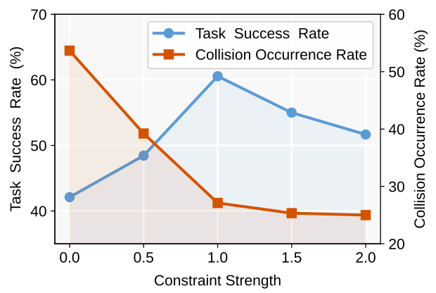
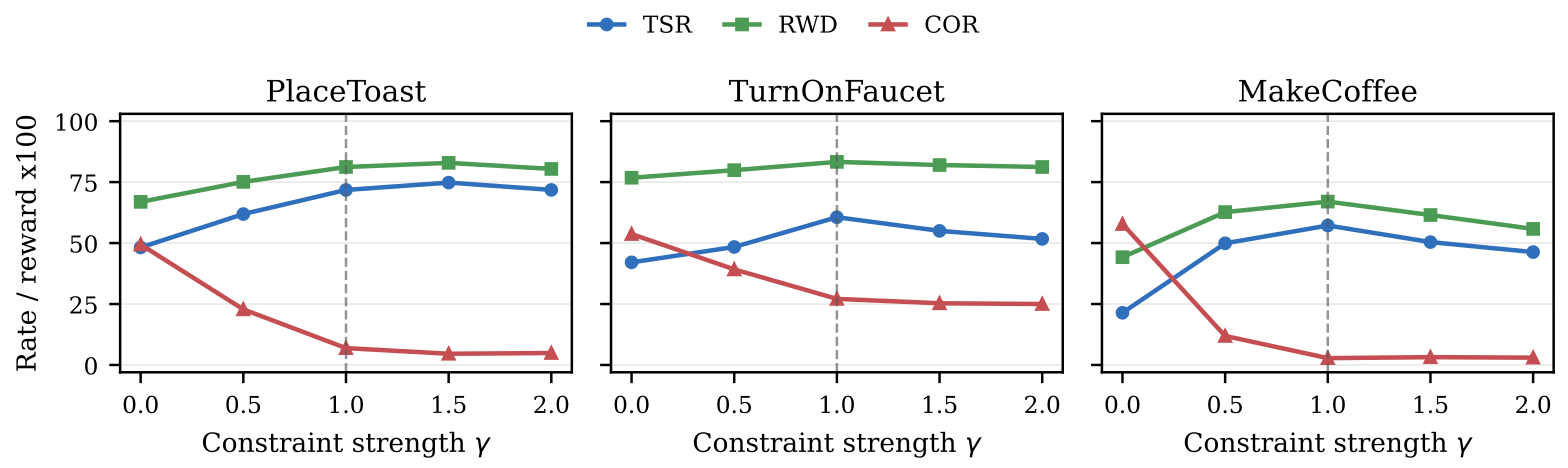
Stronger guidance first reduces collisions but can eventually displace the policy from task-relevant motions. The regularization sweep and scheduled-versus-constant comparison retain this trade-off; MakeCoffee success drops from 57.2% to 46.2% under constant guidance despite equal 2.8% collision rates.
The PlaceToast default in Tables 7–8 is 71.8% success and 6.9% collisions, whereas Tables 1 and 5 give 74.8% and 4.6%. These source values are retained separately rather than silently reconciled. Cost-gradient scale sweeps also show that collision reduction alone need not preserve precise manipulation.
| Task | TSR | RWD | COR | |
| PlaceToast | 0.000 | 70.8% | 0.800 | 5.9% |
| 0.001 | 70.0% | 0.797 | 6.1% | |
| 0.005 | 72.4% | 0.809 | 5.0% | |
| 0.010 | 71.8% | 0.812 | 6.9% | |
| 0.050 | 70.9% | 0.797 | 5.3% | |
| 0.100 | 70.1% | 0.797 | 5.7% | |
| 0.500 | 69.9% | 0.797 | 5.9% | |
| 1.000 | 70.9% | 0.803 | 7.1% | |
| TurnOnFaucet | 0.000 | 57.2% | 0.829 | 26.3% |
| 0.001 | 58.9% | 0.842 | 25.7% | |
| 0.005 | 58.6% | 0.833 | 24.9% | |
| 0.010 | 60.6% | 0.833 | 27.1% | |
| 0.050 | 57.0% | 0.817 | 26.6% | |
| 0.100 | 59.6% | 0.831 | 25.9% | |
| 0.500 | 59.7% | 0.838 | 25.7% | |
| 1.000 | 60.2% | 0.835 | 24.6% | |
| MakeCoffee | 0.000 | 46.3% | 0.603 | 3.6% |
| 0.001 | 42.4% | 0.574 | 3.2% | |
| 0.005 | 45.3% | 0.591 | 2.6% | |
| 0.010 | 57.2% | 0.670 | 2.8% | |
| 0.050 | 47.2% | 0.606 | 2.0% | |
| 0.100 | 42.7% | 0.570 | 3.4% | |
| 0.500 | 44.7% | 0.590 | 3.6% | |
| 1.000 | 46.4% | 0.603 | 3.6% |
| Task | Guidance scale | TSR | RWD | COR |
| PlaceToast | Scheduled | 71.8% | 0.812 | 6.9% |
| Constant | 70.2% | 0.796 | 5.6% | |
| TurnOnFaucet | Scheduled | 60.6% | 0.833 | 27.1% |
| Constant | 57.8% | 0.827 | 26.1% | |
| MakeCoffee | Scheduled | 57.2% | 0.670 | 2.8% |
| Constant | 46.2% | 0.593 | 2.8% |
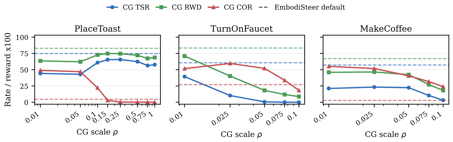
C.5 Obstacle-Present Training and Obstacle-Estimation Noise
Obstacle-present floating-gripper training raises TurnOnFaucet success only 2.4 percentage points over obstacle-free training and remains 16.6 points below guidance; it still contains no deployed-arm body states.
Geometric estimation noise matters. On MakeCoffee, adding 5/10 mm translation-and-extent standard deviation plus 3° rotation noise lowers success from 57.2% to 50.4%/44.6% and raises collisions from 2.8% to 4.4%/6.8%. The physical evaluation assumes known cuboids, not an implemented unknown-obstacle perception system.
C.6 Demonstration Coverage Settings
One sweep retrains with 20, 50, 100 or 200 demonstrations. Another holds 200 demonstrations and scales motion-planner waypoint randomization to 10%, 33%, 67% or 100%. Those percentages measure diversity settings, not fractions of retained demonstrations; both broader coverage and more examples help guided task completion.
C.7 Candidate Sampling Budget
Increasing candidate count from four to thirty-two raises TurnOnFaucet sampling-baseline success from 43.1% to 45.9%, still below EmbodiSteer’s 60.6%. Latency grows from 1.48 to 10.97 seconds per chunk.
Success is averaged across nine arms on TurnOnFaucet, whereas latency is measured separately on PlaceToast/Panda with an RTX 4090. Table 10 preserves both measurement conditions and timing deviations.
C.8 Action-Chunk Continuity
Sixty episodes produce 2,540 paired guided/unguided chunks on Panda and UR5. Each pair shares observation, joints and diffusion randomness, but only the guided chunk executes. The comparison is a trajectory diagnostic, not a matched unguided rollout experiment.
The normalized joint-step 95th percentile changes at most 1.6% in five settings and rises 12.7% on TurnOnFaucet/Panda. Maximum second-difference ratios reach 4.582 on MakeCoffee/UR5 and 2.693 on PlaceToast/UR5, so stable typical steps do not rule out sharper local acceleration changes. Gripper motion is excluded.
| Task | Robot |
P95 step
unguided
|
P95 step
guided
|
Ratio |
QP active
(%)
| |
| MakeCoffee | Panda | 0.0348 | 0.0351 | 1.011 | 1.000 | 10.5 |
| UR5 | 0.0216 | 0.0216 | 0.999 | 4.582 | 28.7 | |
| TurnOnFaucet | Panda | 0.0392 | 0.0442 | 1.127 | 1.000 | 28.8 |
| UR5 | 0.0135 | 0.0135 | 1.003 | 1.292 | 54.5 | |
| PlaceToast | Panda | 0.0244 | 0.0246 | 1.007 | 1.000 | 7.7 |
| UR5 | 0.0171 | 0.0174 | 1.016 | 2.693 | 7.2 |
C.9 Additional Qualitative Results
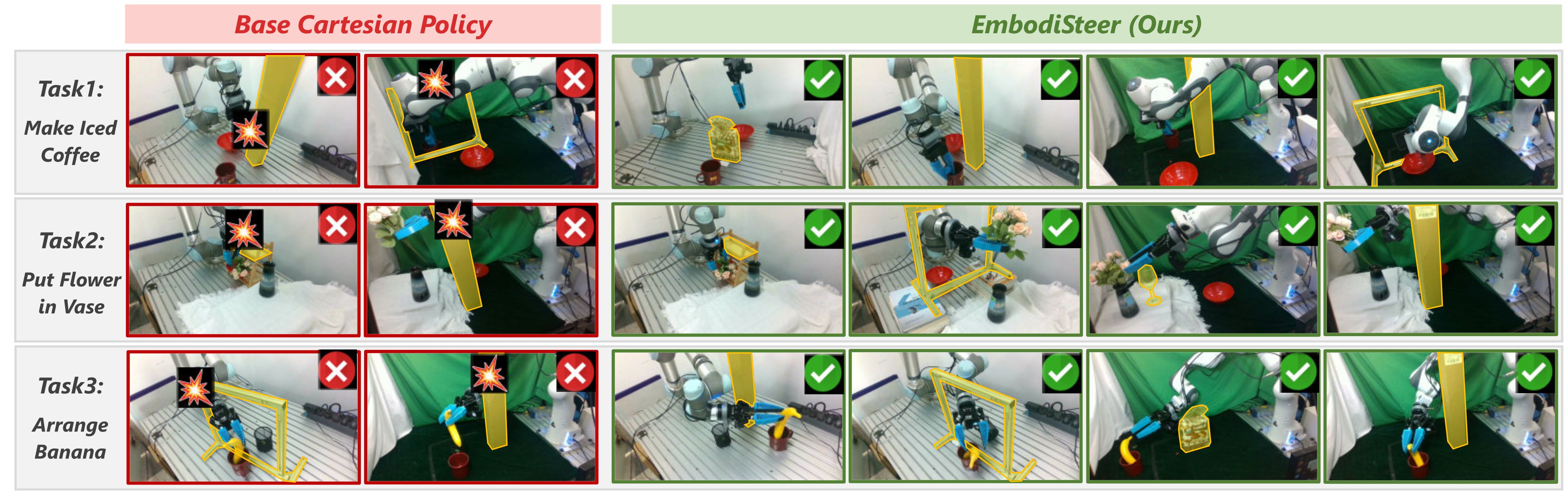
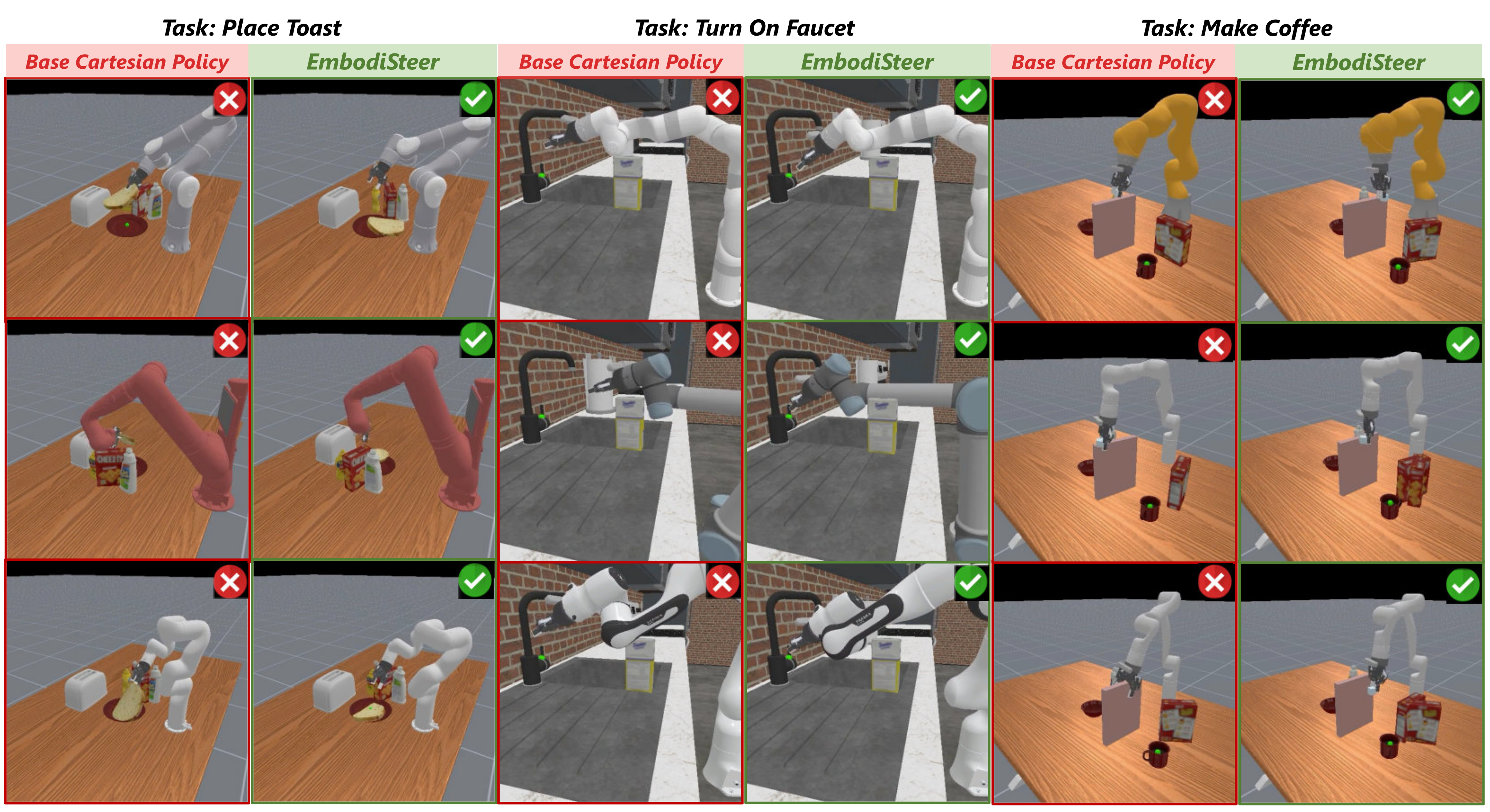
The full simulation sequences contrast end-effector collisions and arm-link collisions under unguided execution with guided examples. They illustrate observed behavior and do not replace the per-robot failure rates.
Appendix D Real-World Results
The physical appendix retains task definitions, independent success/contact annotations, complete trial counts and every qualitative sequence.
D.1 Setup and Annotation Protocol
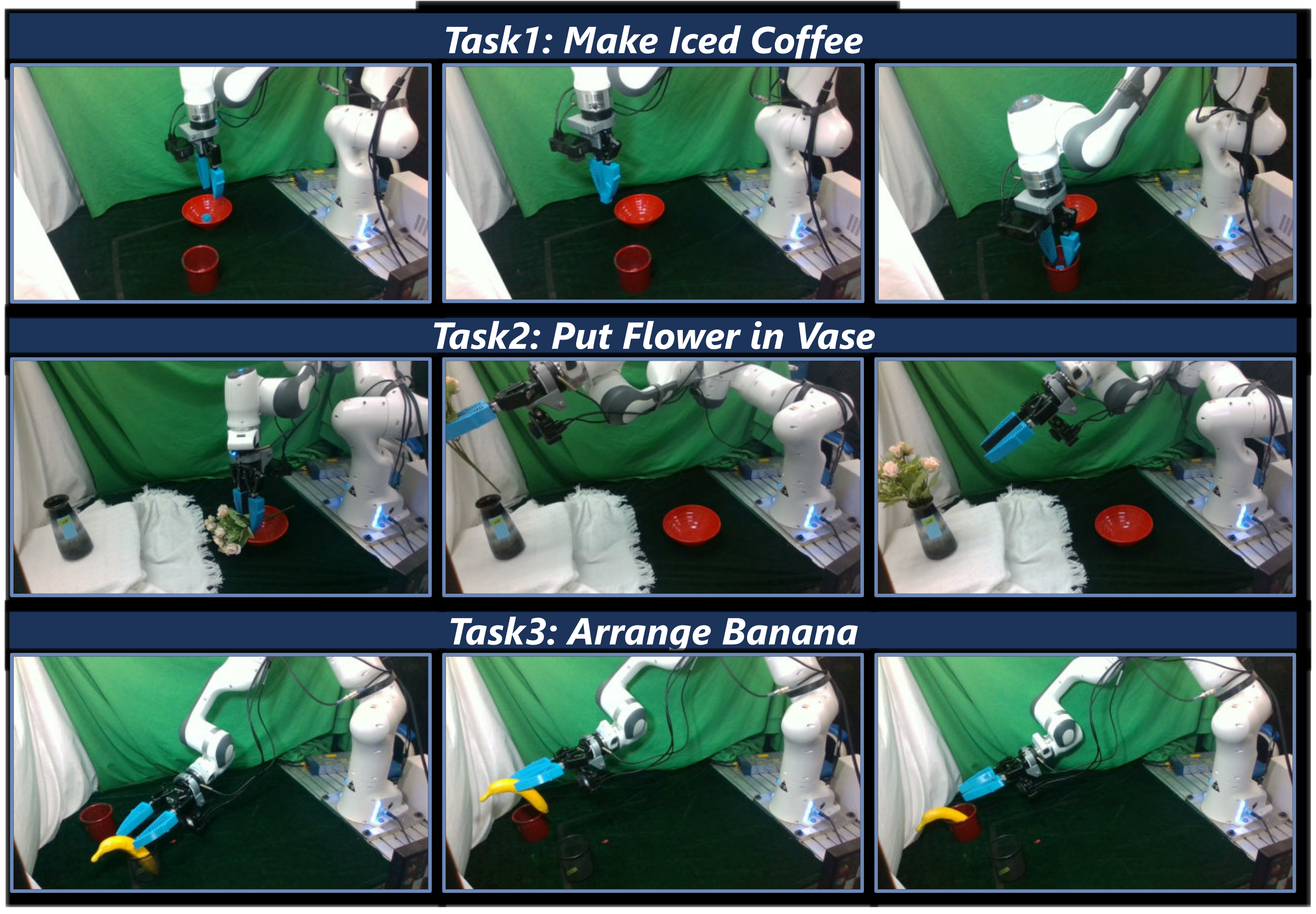
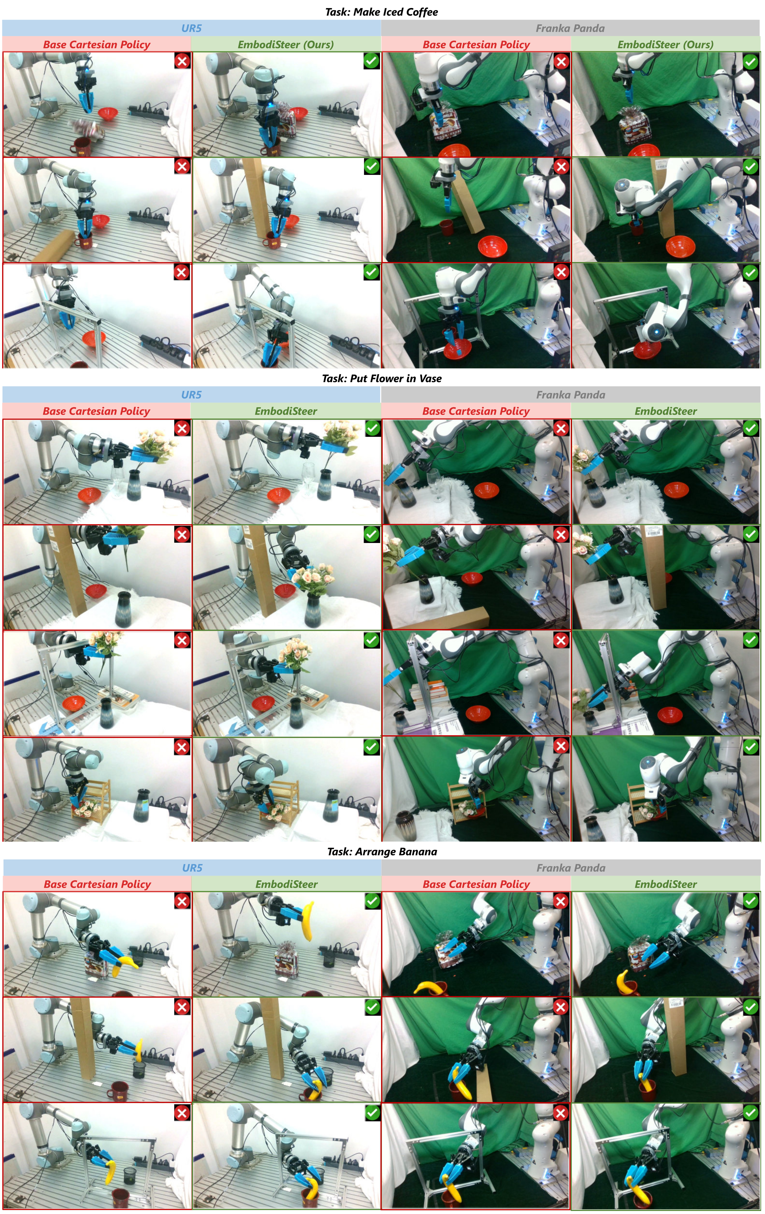
MakeIcedCoffee transfers blocks representing ice from a bowl into a cup; PutFlowerInVase inserts a bouquet; ArrangeBanana moves a banana from a pen holder into a cup. Each task uses 200 UMI demonstrations and one checkpoint shared across UR5 and Panda.
Ten trials per robot-task-setting test final object placement without timeout, dropping or human intervention. Obstacles can move when contacted for safety; a robot may push one aside and still complete the task. Any arm or end-effector contact is counted independently as collision.
D.2 Full Real-World Results
Table 12 keeps every ten-trial numerator and denominator. Guided outcomes range from 6/10 to 10/10 successes, with zero or one collision per robot-task pair. Totals are 47/60 successes and 4/60 collisions; the small task-level samples should not be read as precise estimates of deployment reliability.
| Robot | Task | No Obstacle | Obstacle, Base Policy | Obstacle, EmbodiSteer | ||
| TSR | TSR | COR | TSR | COR | ||
| UR5 | MakeIcedCoffee | 9/10 | 4/10 | 10/10 | 8/10 | 1/10 |
| PutFlowerInVase | 7/10 | 4/10 | 9/10 | 6/10 | 1/10 | |
| ArrangeBanana | 8/10 | 4/10 | 9/10 | 9/10 | 0/10 | |
| Panda | MakeIcedCoffee | 9/10 | 6/10 | 10/10 | 8/10 | 1/10 |
| PutFlowerInVase | 6/10 | 1/10 | 10/10 | 6/10 | 0/10 | |
| ArrangeBanana | 10/10 | 6/10 | 10/10 | 10/10 | 1/10 | |
| Total | All tasks | 49/60 | 25/60 | 58/60 | 47/60 | 4/60 |
D.3 Obstacle Layouts and Qualitative Results
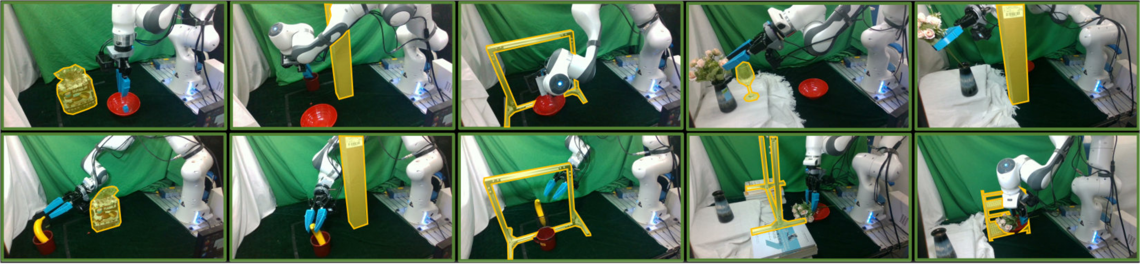
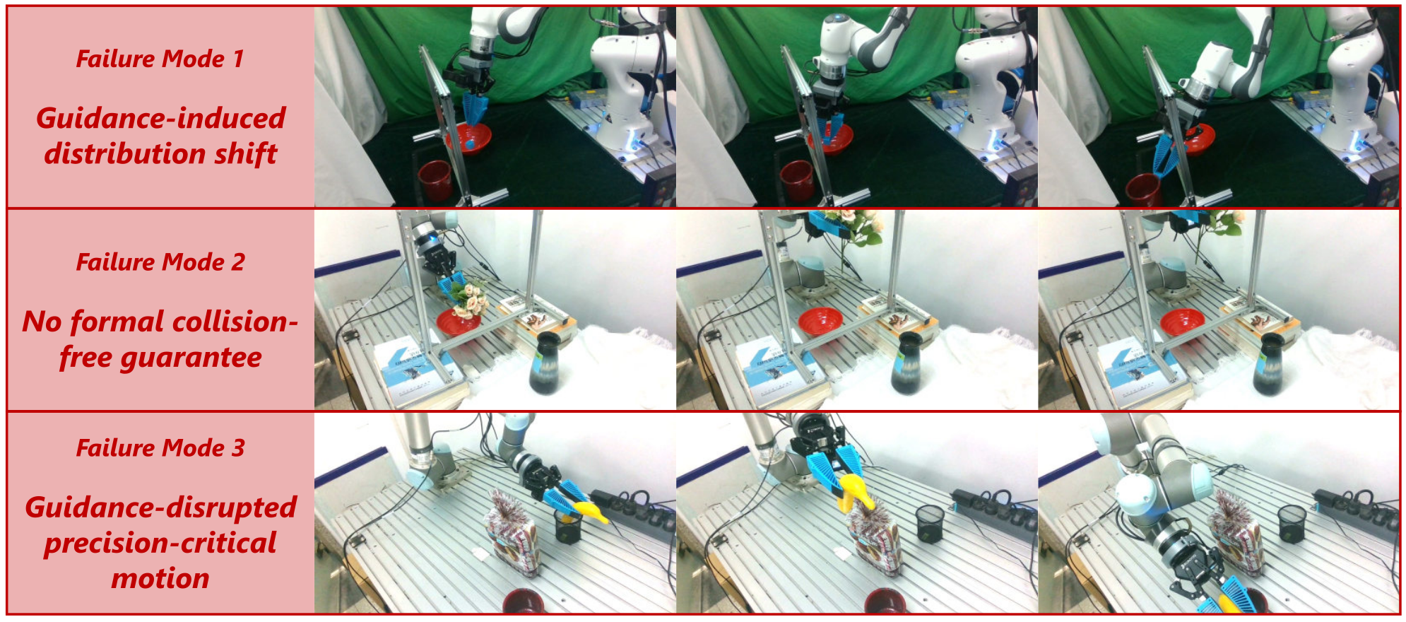
Obstacle type and pose vary across episodes. Figures 15 and 17 preserve the complete layouts and both-robot sequences for all three tasks; Figure 16 records representative failures rather than only successful rollouts.
Appendix E Failure Mode Analysis
Three failure modes remain: corrections can produce observations outside the demonstrations; local, clipped QP steps can leave unavoidable or unresolved contacts; and small gripper deviations can spoil precision-critical grasping or placement. Collision avoidance and task completion remain separate objectives, neither guaranteed by the local guidance rule.