Overview
This edition covers the complete 52-page v1 dated 10 June 2026, including the theoretical proofs, four algorithms and all experimental appendices. The proposed training rule changes when auxiliary data is sampled along the diffusion process; inference retains the ordinary Diffusion Policy procedure.
At a glance
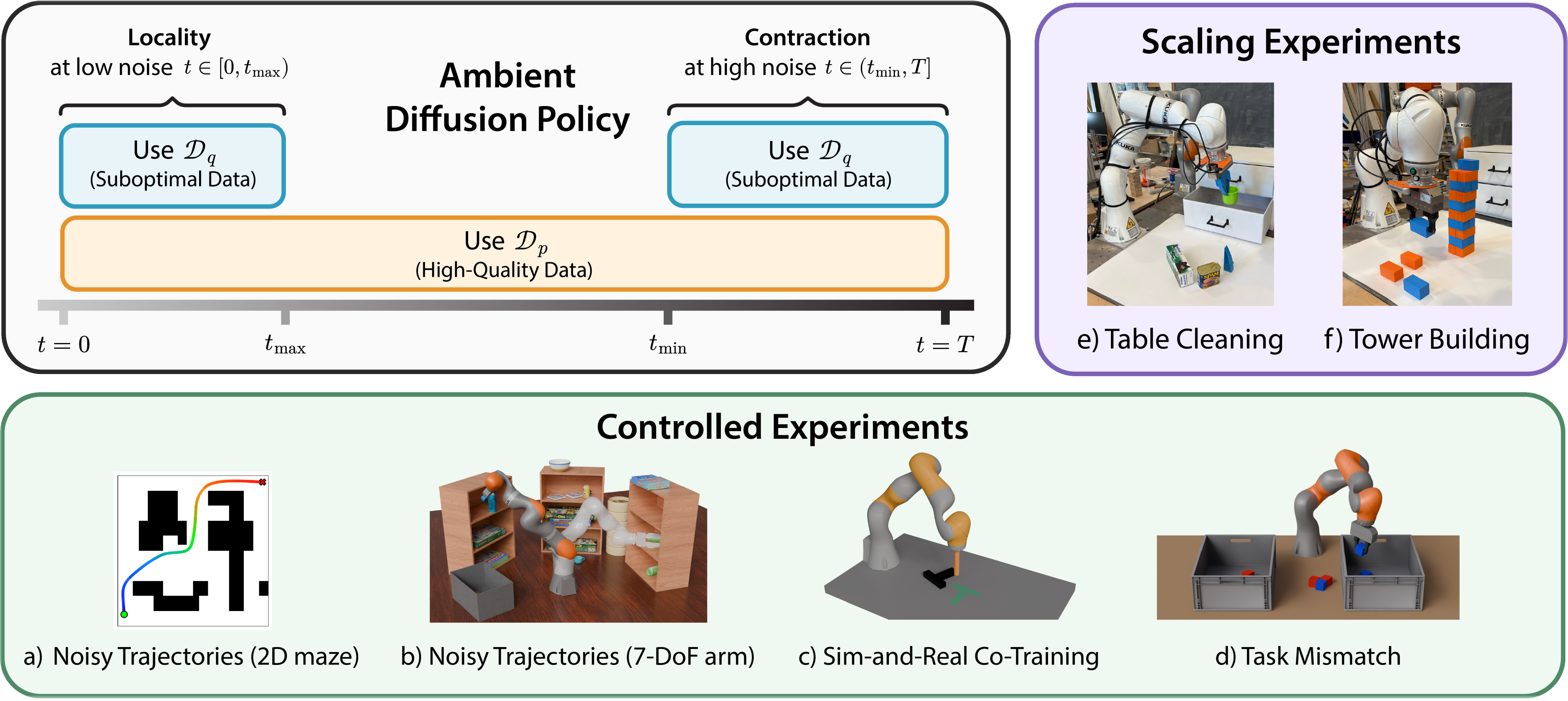
Ambient Diffusion Policy uses a small target dataset together with a larger, imperfect auxiliary dataset. Auxiliary samples contribute only at selected high-noise or low-noise steps, where their global plans or local motion primitives respectively resemble the target data.
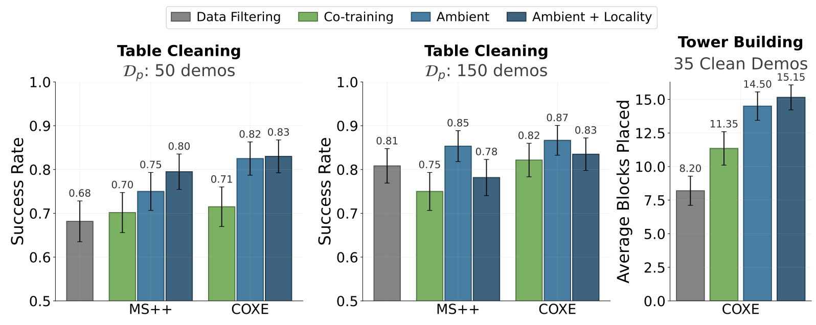
Experiments span noisy planning trajectories, a simulated proxy for sim-to-real transfer, incorrect-task demonstrations and heterogeneous OXE mixtures. The strongest OXE tower result averages 15.15 correct blocks versus 11.35 for co-training, approximately 33% more. Evidence for broader robot-data structure is empirical; the formal analysis uses a simplified stationary Gaussian model.
1 Introduction
Large robot datasets mix tasks, embodiments, control quality and environments. Filtering discards useful structure, while training on every part of a mixture can teach its undesirable behavior. Noise-dependent sampling instead asks which features each source can contribute.
Building on Ambient Diffusion Omni and Diffusion Policy, the paper connects low-frequency action structure to early global planning and high-frequency structure to late refinement. It evaluates selective use of auxiliary data across six tasks, including two physical-robot tasks trained with Open X-Embodiment.
2 Related Work
Dataset re-weighting changes how often a source contributes but ordinarily uses it at every noise level. Filtering rejects entire samples, and finetuning can mitigate mixture bias after pretraining. Ambient is complementary to weights and finetuning because it restricts the learning signal within each diffusion trajectory.
Earlier corrupted-data methods often assume a known corruption or discard suspect examples. Quality conditioning, auxiliary dynamics objectives and invariant representations offer other approaches; this paper focuses on action distributions and does not solve arbitrary observation corruption. OpenVLA’s curated mixture supplies an important scaling baseline.
Equation 1
| (1) |
3 Background
The setup distinguishes the desired conditional action distribution from an auxiliary distribution that may contain different low-level behavior or task structure.
3.1 Robot Imitation Learning and Diffusion Policy
A diffusion policy predicts a future action chunk from recent observations by learning denoisers over increasing Gaussian noise levels. Squared-error training ideally recovers the conditional mean of the clean action, which supports reverse-process sampling.
The exposition uses variance-exploding noise for simpler notation. The actual implementation uses variance-preserving diffusion; Appendix B derives the corresponding rescaling, scores and denoisers.
Equations 2–3
| (2) |
| (3) |
3.2 Problem Setting
The user chooses a small high-quality target set and a larger auxiliary set. Here the target contains expert demonstrations for the desired robot, task and environment. The objective is better target-distribution denoising, rather than faithful imitation of the combined mixture; choosing this partition remains a consequential human design decision.

Selectable problem statement
3.3 Ambient Diffusion Omni
Ambient annotates lower and upper noise cutoffs for auxiliary samples. High noise can erase local discrepancies between target and auxiliary actions, allowing shared global structure to be learned. Low-noise use is separately justified when local primitives agree despite different global tasks.
The retained total-variation contraction bound motivates this idea, but distributional proximity is approximate. The source writes Gaussian covariance with sigma rather than sigma squared immediately after Equation 4; the later formal definitions use sigma squared.
Equation 4
| (4) |
4 Distributional Properties of Robot Data
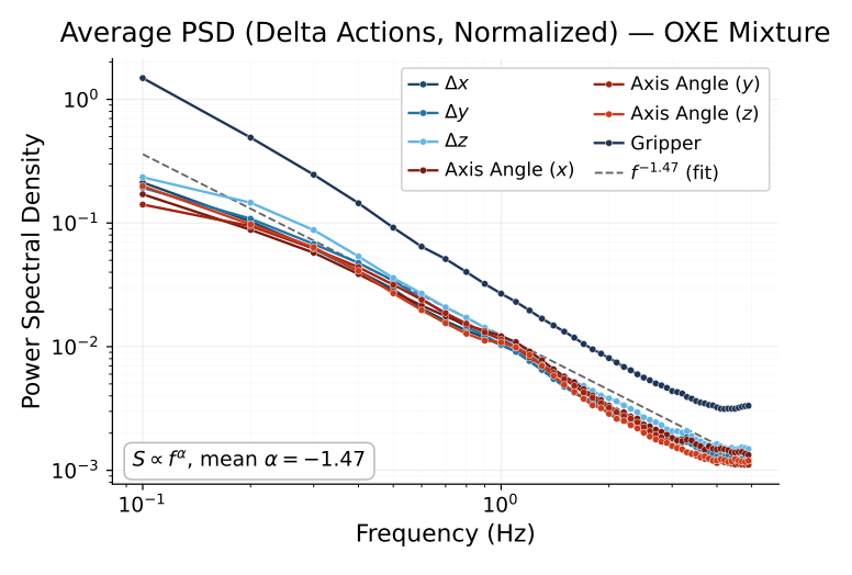
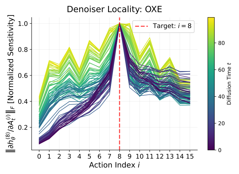
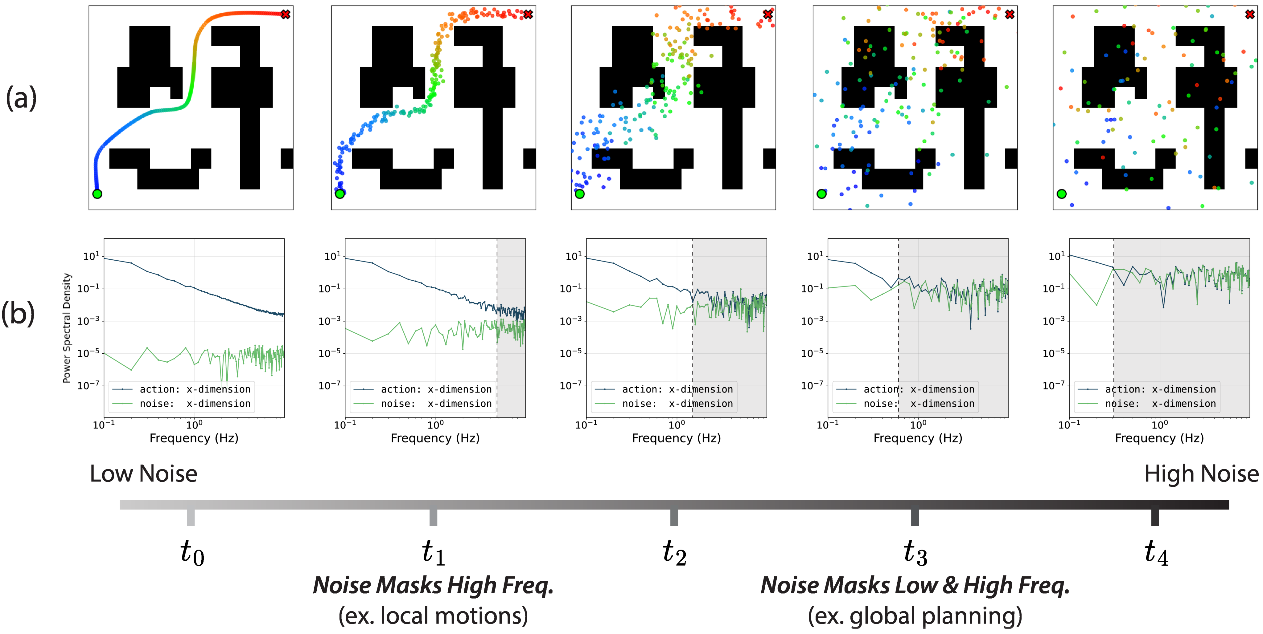
Across the examined datasets, action power concentrates at low temporal frequencies. The paper links this observation to hierarchical denoising and sensitivity concentrated around neighboring actions. These are measured properties of the tested data, not an empirical survey of every possible robot action distribution.
4.1 Spectral Power Law in Robotics
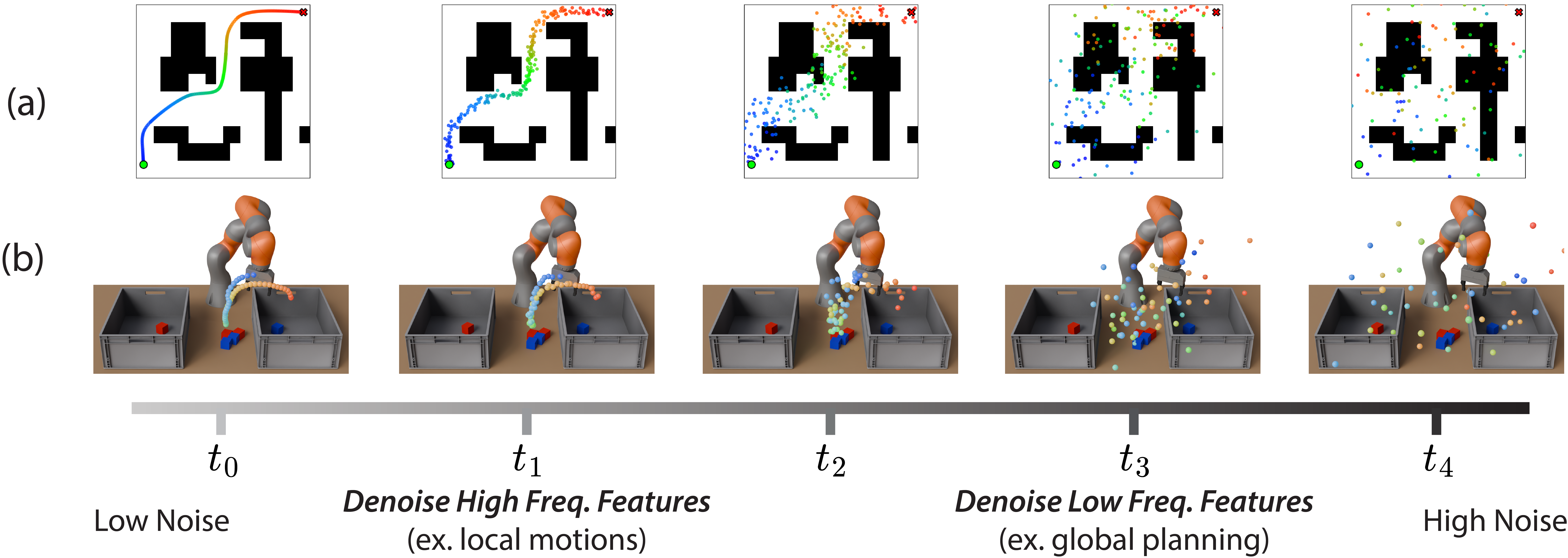
Power spectral density decays approximately as a frequency power law in OXE and six other action datasets. Gaussian noise masks weak, high-frequency details first, leaving global path structure distinguishable at higher noise. Reverse denoising consequently resolves a broad plan before local collision avoidance and smooth motion.
If auxiliary and target data share that broad plan but differ mainly in jitter or contact details, restricting auxiliary use to sufficiently high noise can preserve its coverage without copying its local defects. Figures 2–4 retain the trajectory, spectrum and sensitivity evidence.
4.2 Locality in Robotics
At low noise, the eighth predicted action is empirically most sensitive to nearby noisy actions. This locality suggests that demonstrations with the wrong task-level ordering may still teach useful grasping or motion primitives when admitted only late in denoising.
The argument requires local agreement. It does not imply that every wrong-task sample is harmless at a chosen low-noise cutoff, or that a learned finite-data denoiser exactly equals the theoretical optimal one.
5 Theoretical Foundations
The exact definition and theorem statements below retain their assumptions. The analysis uses zero-mean stationary Gaussians, whose circulant covariance is diagonalized by the Fourier transform; extension to general robot-data distributions is future work.
Equation
Definition 1 (Spectral Power Law).
Let be a zero-mean, stationary random vector on , and let denote its power spectral density in the orthonormal Fourier basis. We say that the distribution of follows a spectral power law if there exist a constant , a rolloff exponent , and a cutoff frequency such that the high-frequency spectrum satisfies:
The exact spectral behavior below the cutoff is permitted to be arbitrary but bounded.
5.1 Contraction Through Noise
When low-frequency spectra agree and the remaining spectral tails obey a power-law bound, sufficiently large Gaussian noise bounds KL divergence as the inverse fourth power of noise scale and total variation as the inverse square. The bounds depend on tail amplitude and cutoff, rather than the original total-variation distance.
This theorem assumes exact low-frequency agreement and a specified minimum noise variance. It supports the mechanism under those conditions, rather than guaranteeing useful transfer from an arbitrary auxiliary dataset.
Equation ⋆
Theorem 1 (Spectral Power Law implies fast contraction through noise).
Let and be zero-mean stationary Gaussians on with power spectra . Fix a cutoff frequency , an exponent , and a constant . Assume:
- 1.
(Low-frequency agreement.) for every .
- 2.
(Power-law tail.) for every such that .
Let and . If

Exact source MathML
| () |
then

Exact source MathML
5.2 Spectral Power Law Implies Locality
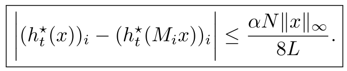
The stated locality result bounds the change in one denoised coordinate after masking distant input coordinates by a term proportional to signal length and amplitude and inversely proportional to neighborhood radius. The appendix derives spatial decay through the Wiener filter.
The displayed final bound has no explicit noise dependence. Moreover, the proof uses a smooth power law from frequency one, whereas Definition 1 permits an arbitrary bounded low-frequency region. These source assumptions and the unchanged bound should be considered when interpreting the broader low-noise locality claim.
Equation
Theorem 2 (Spectral Power Law implies locality of the optimal denoiser).
Let be a zero-mean stationary Gaussian on whose power spectrum follows a spectral power law with constant and exponent . Let be the variance-exploding noisy observation, and denote the MMSE optimal denoiser.
Let be a circulant mask that sets to zero all coordinates of the input at a circular distance strictly greater than from index . Then, for any mask size , the absolute error in the -th coordinate between the full optimal denoiser and the masked denoiser is bounded by:
Exact source MathML
6 Ambient Diffusion Policy: Method
Training has two phases: determine usable noise intervals for auxiliary data, then sample only admissible data at each randomly drawn diffusion time.
6.1 Phase 1: Dataset annotation
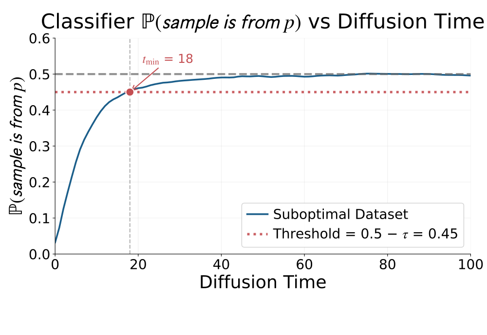
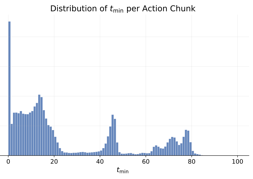
A sweep can choose the cutoffs. Alternatively, train a balanced classifier to distinguish noisy target actions from noisy auxiliary actions and choose the first noise level where its mean prediction on auxiliary data exceeds a threshold near one half.
Labels may be assigned per dataset, per trajectory, per partition or per action chunk. The theoretical guarantee assumes a near-optimal population classifier; finite-data training does not establish that assumption. The classifier here operates on actions and time, so marginal action alignment does not by itself certify observation-conditioned alignment.
Equation 5
| (5) |
6.2 Phase 2: Training
First sample diffusion times uniformly; then sample target data or auxiliary data whose allowed intervals include each time. Target demonstrations remain admissible throughout. The standard denoising objective and inference procedure can remain unchanged.
An optional Ambient loss predicts through an intermediate noisy sample, and a classifier rejection sampler is proposed separately. Most experiments use the ordinary loss; the rejection-sampling variant is theoretically motivated but experimentally untested.
7 Controlled Experiments
Controlled experiments isolate noisy trajectories, simulator mismatch and incorrect task logic. Baselines include target-only filtering, weighted co-training and finetuning; the appendix retains data generation, selection and evaluation details.
7.1 Noisy Trajectories
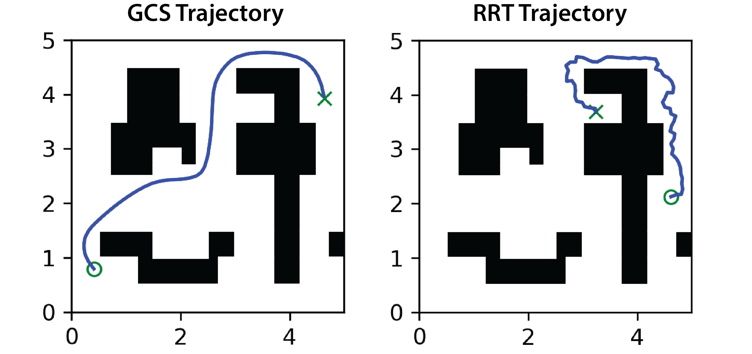
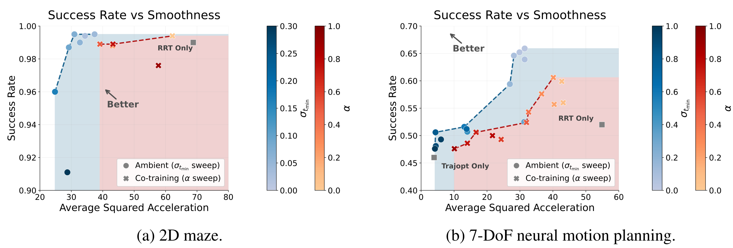
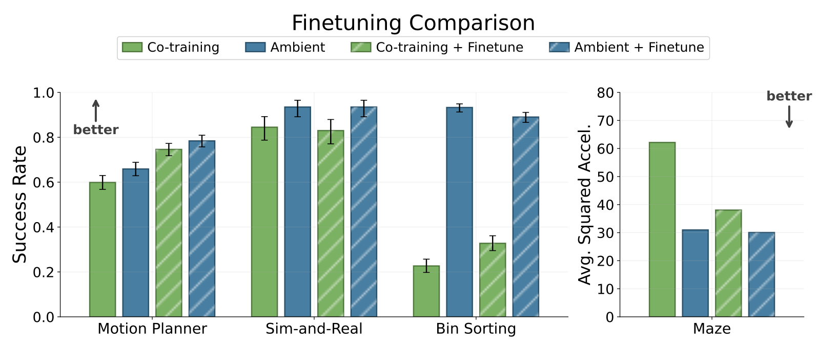
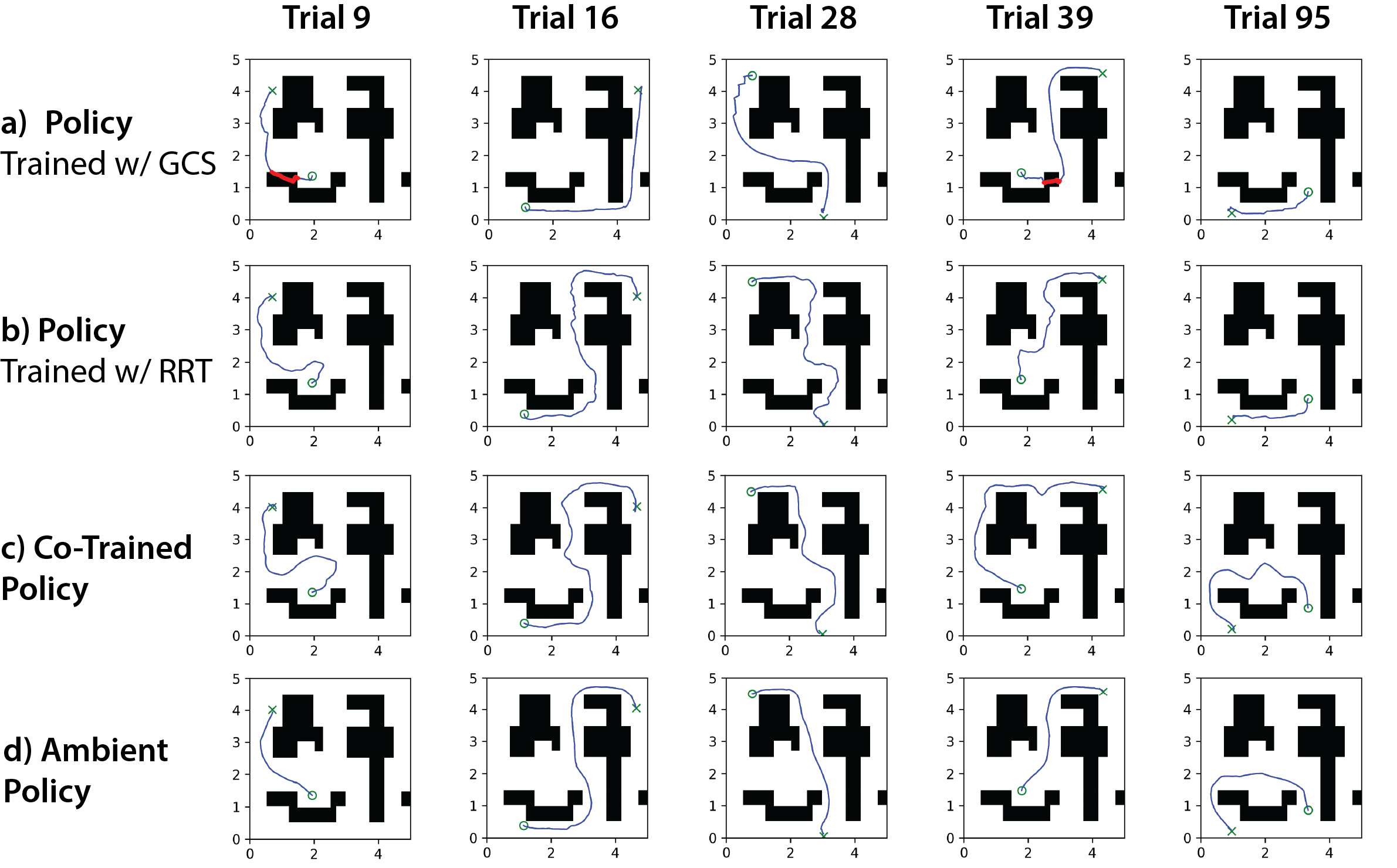
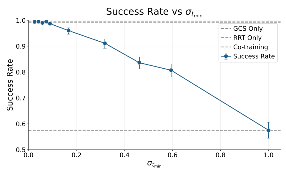
A two-dimensional maze uses 50 smooth GCS trajectories and 5,000 jittery RRT trajectories. Across 1,000 trials, Ambient and co-training reach similar success, 99.5% and 99.4%, while Ambient’s squared-acceleration metric is 31.0 versus 62.2. Target-only training succeeds 57.5% of the time.
Using only auxiliary data above the cutoff and only target data below it still reaches 99.0% success with smoothness 29.9. This supports the separation of global coverage and local motion quality in this task. Smoothness statistics include successful rollouts only.
7.2 Neural Motion Planning
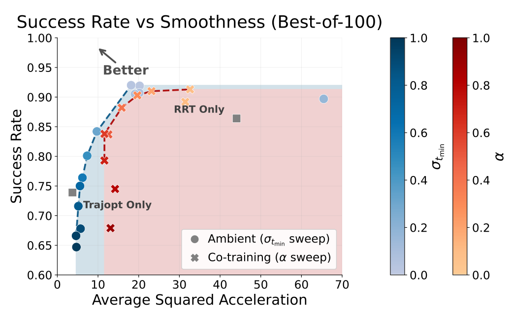
The seven-joint planning task uses 100,000 optimized trajectories and one million BiRRT trajectories. For one predicted full plan per query, Ambient achieves 65.9% success versus 59.9% for co-training, with squared acceleration 31.4 versus 42.7; filtering is smoother but succeeds only 46.0%.
These are open-loop simulated plans. Evaluation accepts up to 2 cm penetration and endpoint error within a .2-radian ball; its success metric therefore does not establish strict collision-free execution on hardware. Best-of-100 selection is reported separately.
7.3 Sim-to-Real Distribution Shift
Planar pushing uses 50 target-simulator teleoperation demonstrations and 2,000 source-simulator planned demonstrations from the earlier sim-and-real study. The two simulators differ visually, dynamically and in action generation, providing a controlled proxy for a sim-to-real gap.
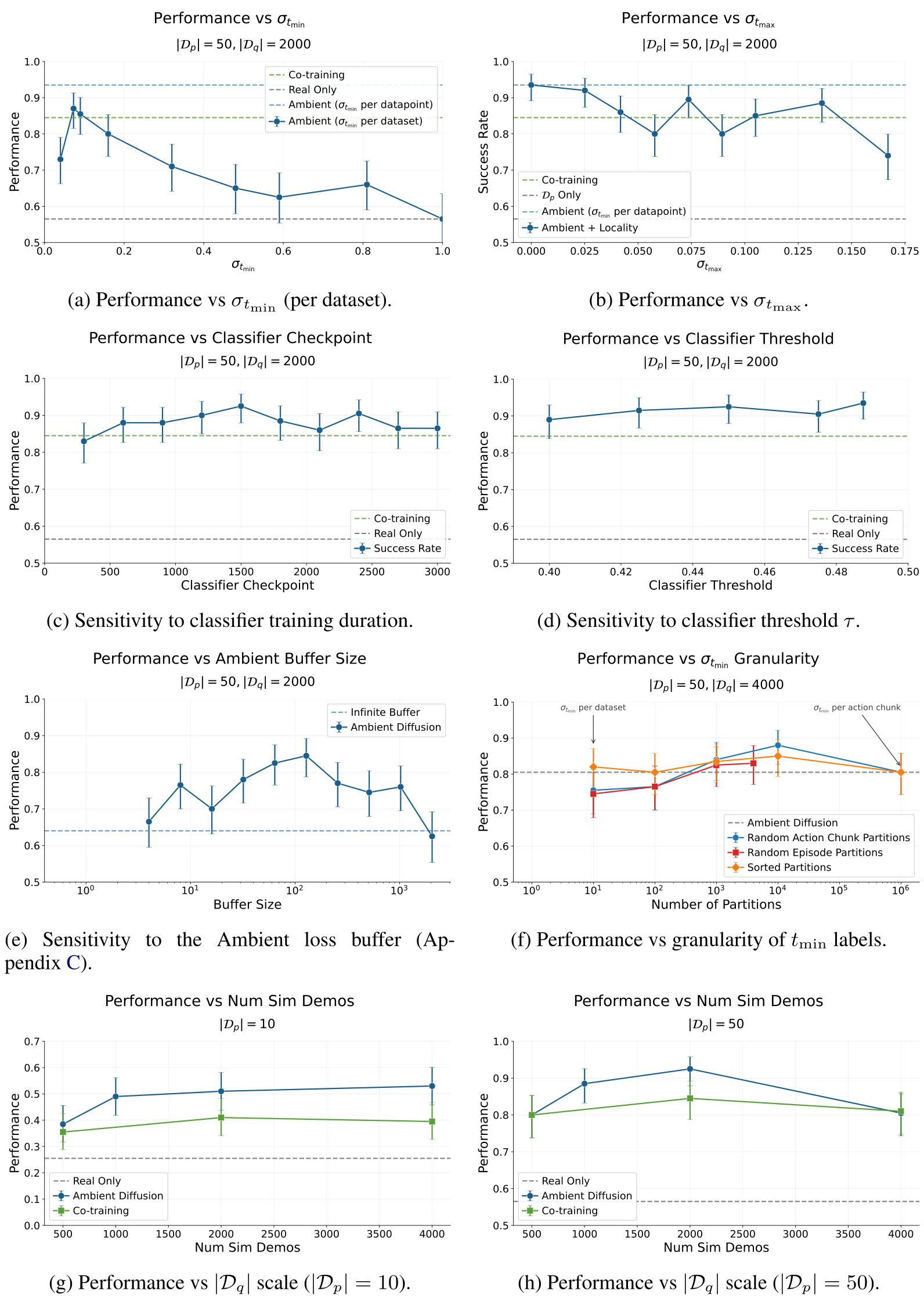
Across 200 trials, per-datapoint cutoff annotation reaches 93.5% success versus 84.5% for co-training and 56.5% for filtering. Per-dataset annotation reaches 87.0%; adding low-noise auxiliary use gives 92.0%, consistent with little benefit when local contact dynamics differ.
7.4 Task Mismatch
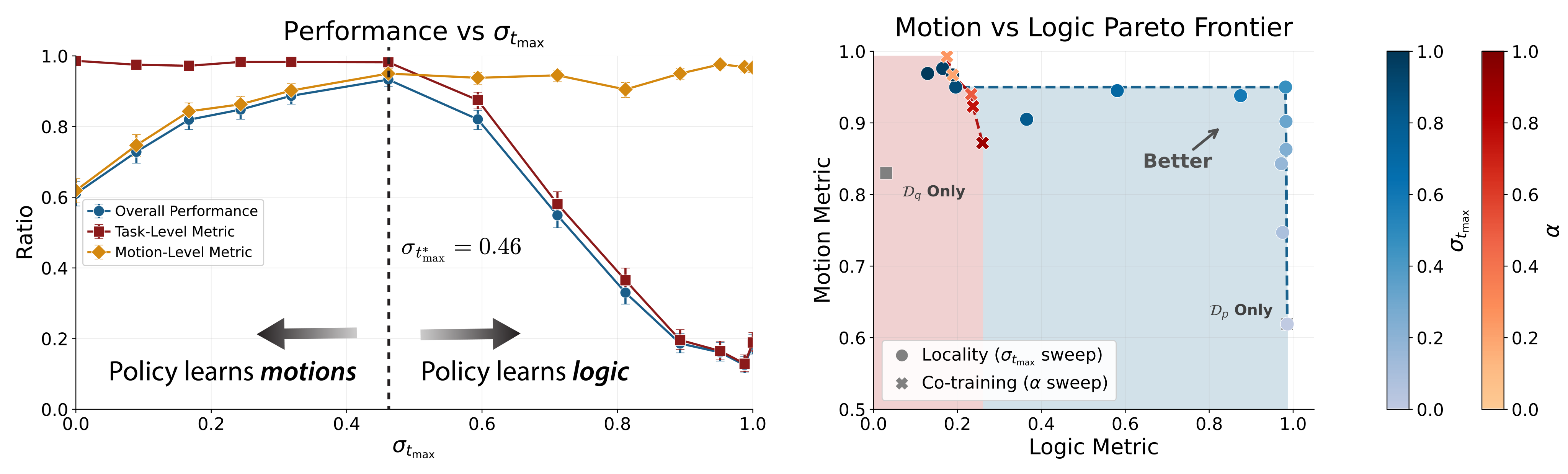
The target set contains 50 demonstrations sorting colors into the correct bins, while 200 auxiliary demonstrations reverse the rule. Low-noise-only auxiliary use reaches 93.3% correctly placed blocks versus 22.7% for co-training and 61.0% for filtering, over about 800 blocks.
Motion success counts blocks placed in either bin; logic accuracy is conditional on a successful placement. Their product is overall correctness. Ambient retains 98.2% conditional logic and 95.0% placement success; task-conditioning and disjoint-noise ablations appear in Appendix G.4.
The text says to set the lower cutoff to zero while isolating low-noise use, which conflicts with its union-of-intervals rule: a zero lower cutoff would also admit all positive high-noise times. The described experiment instead uses auxiliary data only below the upper cutoff; the source wording is retained as a specification inconsistency.
|
Training Algo.
|
Data Filtering
|
Only
|
Co-train
()
|
Locality
()
|
| Logic | % | % | % | % |
| Motion | % | % | % | % |
| Success Rate | % | % | % | % |
7.5 Finetuning Comparison
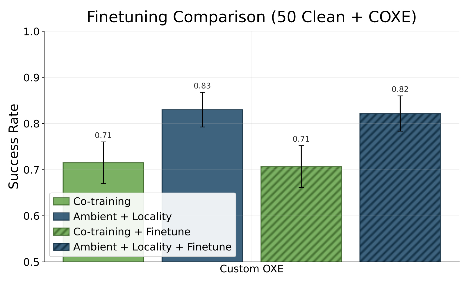
Finetuning the best co-trained and Ambient checkpoints on target data generally favors starting from Ambient. The unfinetuned Ambient policy can already outperform a finetuned co-trained policy, and further target-only finetuning does not consistently help Ambient. These comparisons include checkpoint selection, as detailed in Appendix I.
8 Scaling Experiments: Open X-Embodiment
The physical-robot scaling tasks are drawer-based table cleaning and building alternating-color, alternating-orientation block towers. Target sets contain 50 or 150 cleaning demonstrations, or 35 tower demonstrations. Auxiliary data expands from 27-dataset Magic Soup++ to a 48-dataset custom OXE subset.
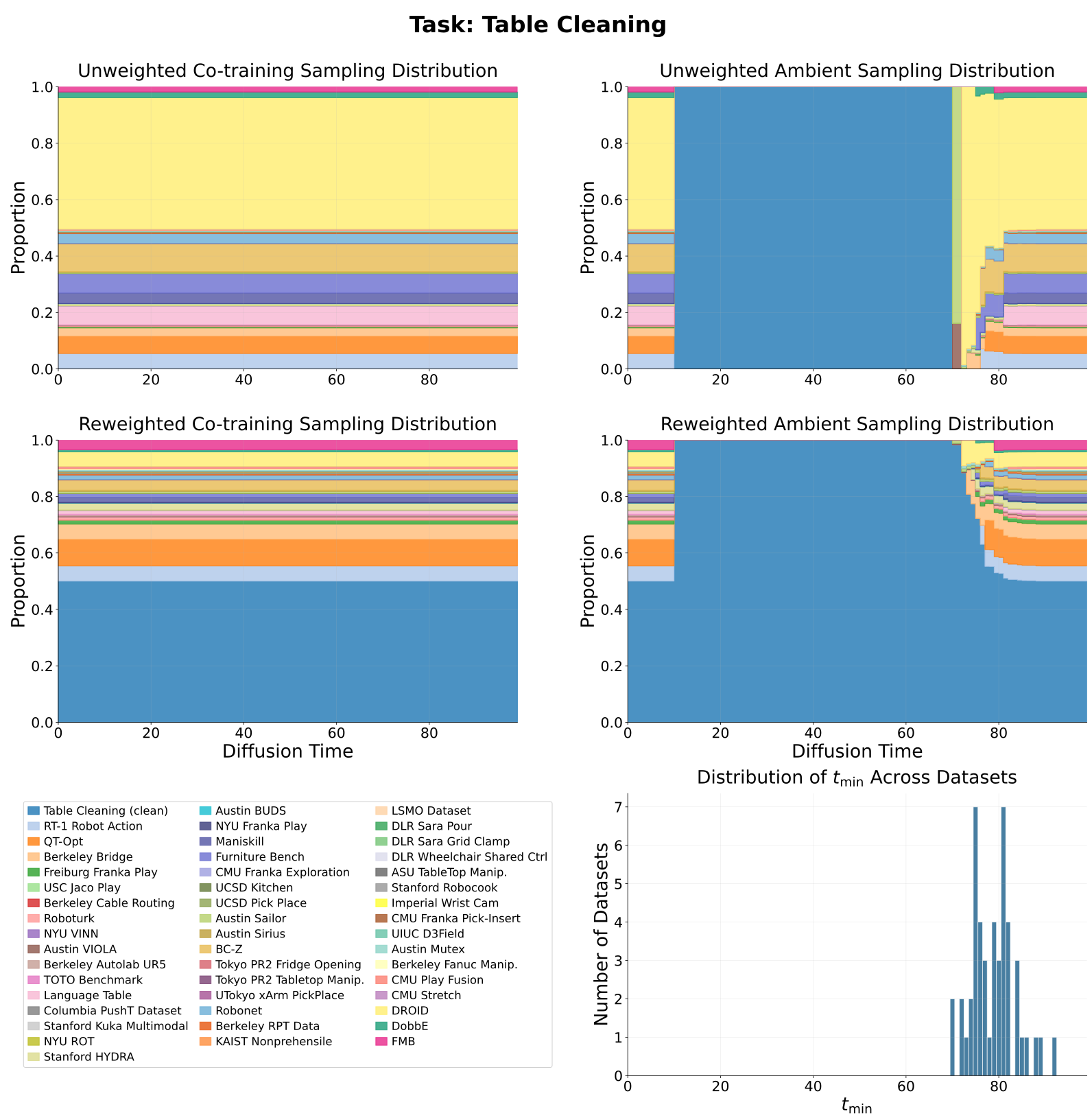
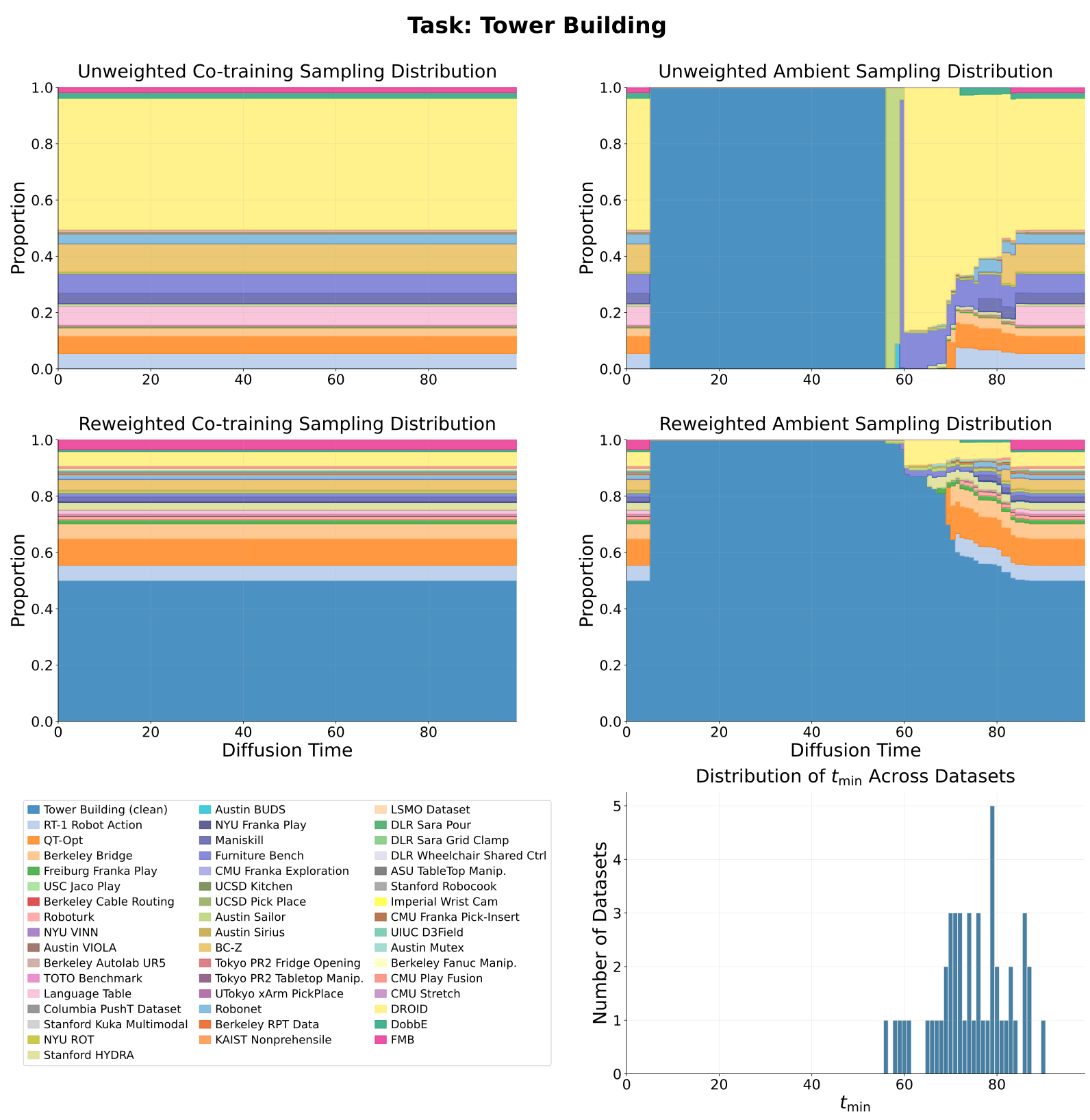
Per-source weights are renormalized among datasets admissible at each noise time. Co-training keeps its mixture fixed over time; Ambient changes the mixture as source cutoffs become active. This makes source weighting and interval selection distinct controls.
Equation 6
| (6) |
8.1 Main Results
With 50 cleaning demonstrations, Figure 9 shows approximately .83 completion for the strongest custom-OXE Ambient variant versus .71 for co-training and .68 for filtering. With 150 demonstrations, the strongest plotted Ambient score is .87 versus .82 for custom-OXE co-training; the value of auxiliary data is smaller.
Tower building averages 15.15 correct blocks for Ambient with locality, versus 11.35 for co-training and 8.20 for filtering, about 33% and 85% relative increases. Each policy receives 20 trials. Percentage changes in the prose mix completion-point differences and relative tower-height changes; the original plots retain the actual values.
8.2 Ablations
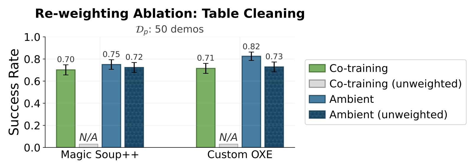
Removing dataset weights lowers the tested Ambient cleaning scores by roughly .03–.09. Unweighted co-trained policies were judged too unsafe to evaluate on hardware, so their plot entries are unavailable, not measured zero success.
Additional measurements cover grasp attempts, time per object and finetuning. Reduced sensitivity in these experiments is useful practical evidence, but does not imply arbitrary mixture weights are safe or irrelevant.
9 Limitations and Future Work
Observation-space shifts remain unresolved. Cutoff classifiers are imperfect and can lose to expensive sweeps; the Gaussian theory is limited, and training on more data costs more than filtering. Choosing the target/auxiliary partition remains essential.
Generalist pretraining would require a principled target definition beyond one task and environment. Better annotation, broader theory and learning from imperfect finetuning data are proposed directions.
10 Conclusion
The central contribution is noise-dependent access to auxiliary demonstrations. The tested cases show that retaining useful global or local structure can improve the trade-off between task success and behavior quality, while the appendix records the assumptions, implementation choices and negative results that limit that conclusion.
Acknowledgments
The authors acknowledge discussions and hardware assistance, NSF and NSERC graduate support, and MIT Supercloud compute.
Appendix A Ambient Diffusion: Theoretical Foundations
This appendix proves the two Gaussian spectral results and analyzes the classifier threshold. All displayed derivations and exact theorem/proposition statements remain available below.
Preliminaries.
The preliminaries define total variation, chi-squared divergence and a LeCam quantity. There is a normalization inconsistency: the printed total-variation definition lacks the one-half factor used later in the rejection-sampling proof, while the stated Pinsker constant follows the latter convention. The original definitions and inequalities are preserved.
Equations
A.1 Spectral Power Law implies fast contraction through noise
Fourier diagonalization reduces Gaussian KL divergence to a sum of spectral variance ratios. Low-frequency agreement removes those terms; the noise lower bound keeps each remaining ratio at least one half, allowing a quadratic bound on the logarithmic expression.
Summing the squared power-law tail and bounding it by an integral yields the inverse-fourth-power noise dependence. Pinsker then gives the stated total-variation estimate. The derivation relies on stationarity, spectral agreement and the tail/noise assumptions throughout.
Equations 7–35
| (7) |
| (8) | |||
| (9) | |||
| (10) |
| (11) |
| (12) | |||
| (13) |
| (14) | |||
| (15) | |||
| (16) |
| (17) | |||
| (18) | |||
| (19) |
| (20) | |||
| (21) |
| (22) |
| (23) |
| (24) |
| (25) |
| (26) |
| (27) |
| (28) |
| (29) |
| (30) | |||
| (31) | |||
| (32) | |||
| (33) | |||
| (34) | |||
| (35) |
A.2 Spectral Power Law implies locality
The Gaussian conditional mean is a circulant Wiener filter. Masking distant coordinates leaves a convolution tail; two finite differences in frequency relate that tail to the total variation of the filter’s slope. A power-law slope estimate gives inverse-square kernel decay and an inverse-radius masking-error bound.
The proof treats a smooth power law from frequency one, without separately bounding the arbitrary low-frequency part permitted by the definition. Its final upper bound also retains a factor of signal length and omits explicit noise dependence. The edition preserves the argument as published rather than strengthening its scope.
Equations 36–58
| (36) |
| (37) |
| (38) | |||
| (39) | |||
| (40) |
| (41) |
| (42) |
| (43) |
| (44) |
| (45) |
| (46) |
| (47) |
| (48) |
| (49) |
| (50) |
| (51) |
| (52) |
| (53) |
| (54) |
| (55) |
| (56) |
| (57) |
| (58) |
A.3 Theoretical Justification of the Classifier-Based Annotation
The classifier analysis uses balanced source priors and population cross-entropy. A classifier’s mean target probability on auxiliary samples is linked to a divergence between the distributions, with an additional error term for approximate optimization.
Classifier threshold implies distributional closeness.
For an optimal balanced classifier, the density ratio determines its prediction; cross-entropy excess risk then bounds the deviation of an approximate classifier. The source states a LeCam upper bound of twice the threshold tolerance plus twice the square root of excess risk.
The printed LeCam definition and Theorem 3’s coefficient are inconsistent. With LC defined as twice chi-squared divergence from the mixture, direct substitution gives one-half minus LC/4 for the mean classifier output, while the source prints LC/2. The theorem constants and proof are retained unchanged and should not be treated as independently verified guarantees.
Equations 59
| (59) |
Theorem 3 (Optimal classifier threshold implies distributional closeness).
Theorem 4 (Approximate classifier threshold implies distributional closeness).
Suppose is an -optimal classifier, i.e. . Then implies .
Appendix B Variance-Preserving vs Variance Exploding Diffusion Processes
Dividing a variance-exploding sample by its time-dependent standard-deviation scale yields the variance-preserving representation with the same signal-to-noise ratio. The density change of variables gives the score scaling, and Tweedie’s identity relates the corresponding optimal denoisers. All three propositions and Equations 60–69 are retained.
Equations 60–69
| (60) | ||||
| (61) |
| (62) |
| (63) |
| (64) |

Exact source MathML
| (66) |
Proposition 3.
| (68) | ||||
| (69) |
Appendix C VP Ambient Loss Derivation
The optional Ambient objective targets an intermediate noisy sample without requiring a clean prediction target. A double-Tweedie identity gives affine relationships for either noise prediction or clean-sample prediction; rescaling yields the two variance-preserving losses with the same ideal denoiser minimizer.
At a zero lower cutoff they reduce to ordinary diffusion MSE. Near the lower cutoff, coefficients diverge, so a buffer rejects unstable time/sample combinations. This buffer is sensitive in the pushing ablation; most experiments therefore use the ordinary loss.
Equations 70–82
Proposition 4.
| (71) |
| (72) |
| (73) | ||||
| (74) | ||||
| (75) |
| (76) |
| (77) |
Proposition 5.
| (79) | ||||
| (80) |
| (81) |
| (82) |
Appendix D Characterization of Robot Action Data and Action Diffusion
PSD measurements normalize action ranges, use 100-step chunks and average per-dimension periodograms. OXE uses 2nd/98th percentile scaling and is converted to 10 Hz by downsampling faster sources and speeding up slower ones; DC is omitted. These preprocessing choices matter when interpreting the observed spectra.
Table 4 retains seven dataset descriptions and fitted slopes. The source says nine-dimensional rotation entries lie in [0,1], although rotation-matrix entries generally span [−1,1]; the actual stated choice is to leave those dimensions unnormalized.
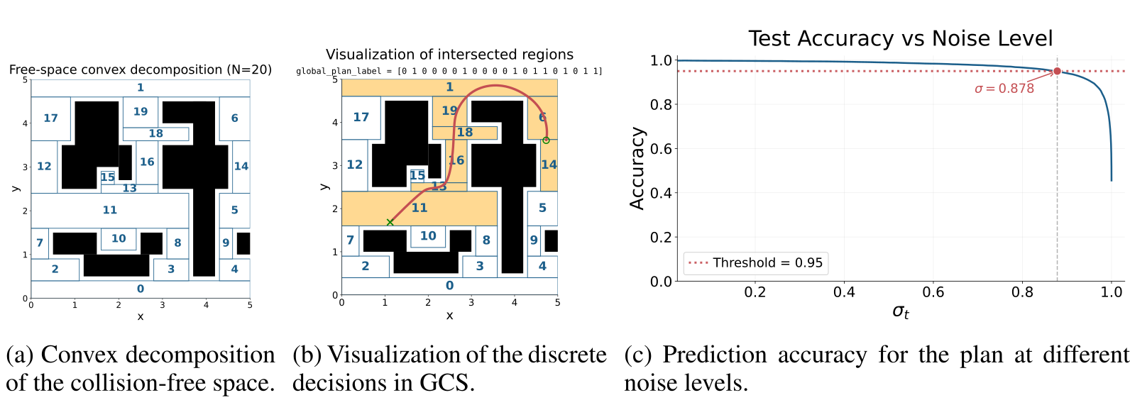
A classifier trained on 5,000 maze trajectories predicts which of 20 convex regions a noisy path visits, excluding start/goal conditioning. It reaches 95% accuracy by noise .878, supporting early recovery of global path information. Equation 83 separately measures normalized Jacobian sensitivity of the eighth action to all sixteen input actions; normalization removes absolute scale differences across noise levels.
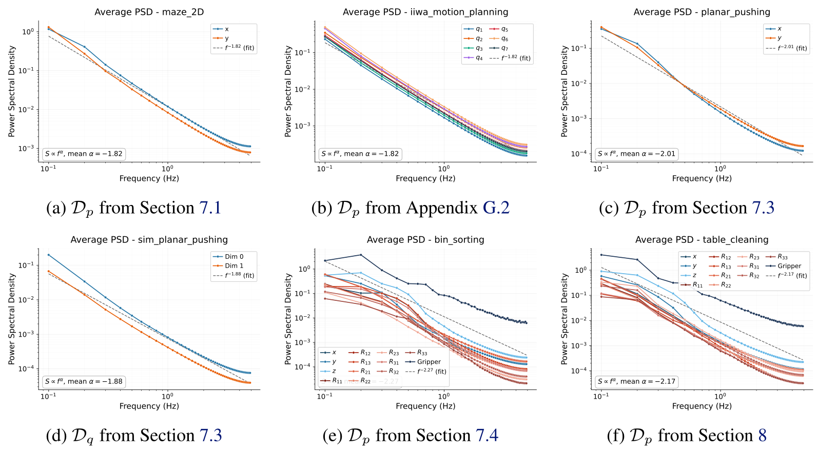
| Fig. | Dataset | Source | Generation | Action Space | Action Type | Rotation Rep. | |
| Fig. 3(a) | COXE [1] | (Sec. 8) | Mixed | Task space | Delta | Axis-angle | -1.47 |
| Fig. 11(a) | GCS [65] | (Sec. 7.1) | Algorithmic | - | Absolute | N/A | -1.82 |
| Fig. 11(b) | TrajOpt. | (App. G.2) | Algorithmic | Joint space | Absolute | N/A | -1.82 |
| Fig. 11(c) | Planar pushing [12] | (Sec. 7.3) | Human teleop | - | Absolute | N/A | -2.01 |
| Fig. 11(d) | Graesdal et al. [72] | (Sec. 7.3) | Algorithmic | - | Absolute | N/A | -1.88 |
| Fig. 11(e) | Block sorting | (Sec. 7.4) | Human teleop | Task space | Absolute | -2.27 | |
| Fig. 11(f) | Table cleaning | (Sec. 8) | Human teleop | Task space | Absolute | -2.17 |
: mean fitted exponent across action dimensions, where
Selectable original panel labels
(a) Convex decomposition of the collision-free space.
(b) Visualization of the discrete decisions in GCS.
(c) Prediction accuracy for the plan at different noise levels.
Equation 83
| (83) |
Appendix E Pseudocode and Possible Extensions
The implementation appendix retains the complete training and loss pseudocode, followed by an untested classifier rejection-sampling extension.
E.1 Ambient Diffusion Policy Pseudocode
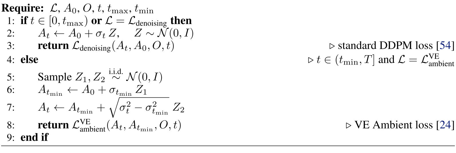
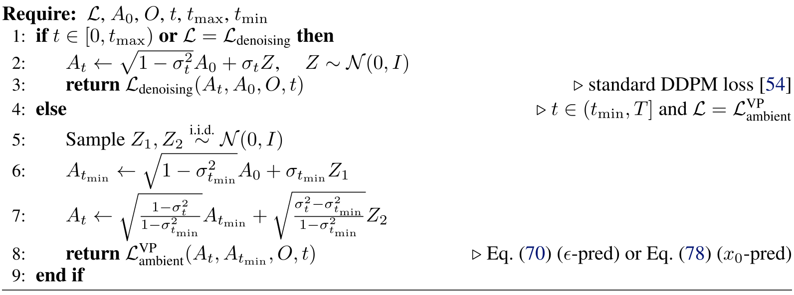
Algorithm 1 samples times before admissible examples. Algorithms 2 and 3 implement variance-exploding and variance-preserving forward processes, using ordinary denoising at low noise and optionally the Ambient objective above the lower cutoff. The source’s first listing line is a Require declaration in the PDF, not an executed numbered operation.
Only the maze experiments use the Ambient loss in the reported main configurations. Testing it on OXE found no significant difference, so the ordinary loss was retained for simplicity.
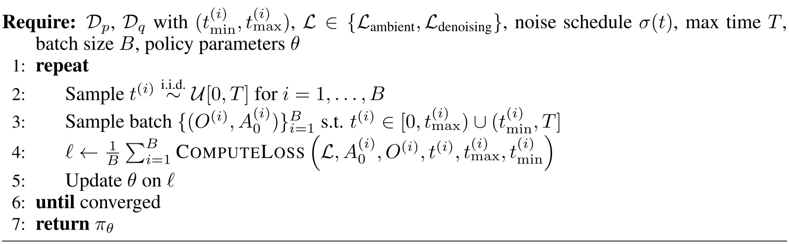
Selectable pseudocode
E.2 Diffusion Policy Implementation Details
Unless otherwise specified, a U-Net predicts sixteen actions at 10 Hz from two observations, executes eight and replans. Image-conditioned policies use ResNet18. Training uses a cosine learning-rate schedule, 100 cosine-scheduled diffusion steps and exponential moving averages; inference uses ten DDIM steps.
Predictions are linearly interpolated and passed through a first-order low-pass filter before execution. The neural motion planner instead predicts a complete 100-waypoint plan, as specified in its task appendix.
E.3 Future Direction: Classifier-Based Rejection Sampling
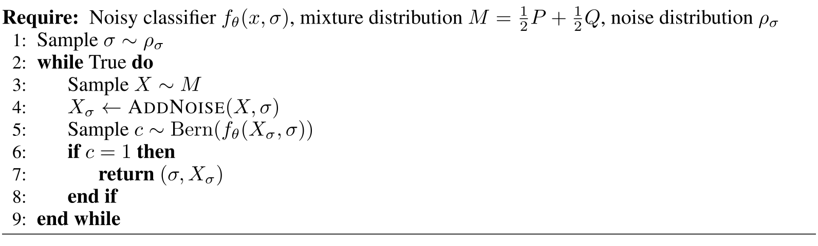
Algorithm 4 samples an equal target/auxiliary mixture, adds noise and accepts according to the classifier’s target probability. With uniformly small population cross-entropy error at each noise level, the proof bounds rejection-sampled distribution error by an order-square-root term.
The proof controls acceptance probability around one half and requires sufficiently small error for the explicit constant. This variant has no experimental validation in the paper; it is not the sampler used for the reported main results.
Selectable pseudocode
Equations
Proposition 6 (Rejection sampling guarantee).
Suppose is uniformly -optimal across :
For any , let be the noisy distribution of , and let be the distribution of output by Algorithm 4. Then
Appendix F Experiments Overview
Tables 5–6 retain every dataset size, observation/action specification, cutoff, mixture weight, prediction target and trial count. Binary outcomes use 95% Clopper–Pearson intervals; other bars are standard errors. Five to ten checkpoints are saved per run and the best-performing checkpoint is reported.
These intervals describe evaluation outcomes rather than independent training-seed uncertainty. Hyperparameters are swept for controlled baselines; OXE uses fixed .5 mixture weighting and manually selected low-noise cutoffs without a hardware sweep.
| Maze |
Neural
Motion Planning
|
Sim-and-Real
Co-training
|
Block
Sorting
| ||
| Dataset Details | GCS [65] |
Trajectory
Optimization [83]
|
Joystick
Teleop [12]
|
VR Teleop | |
| RRT [66] | BiRRT [84] |
Contact-Rich
Planner [72]
|
VR Teleop | ||
| (Num. Demos.) | 50 | 100,000 | 50 | 50 | |
| (Num. Demos.) | 5000 | 1,000,000 | 2000 | 200 | |
| Nature of shift |
Low-quality/
noisy trajectories
|
Low-quality/
noisy trajectories
|
Sim-to-real
gap
|
Task
mismatch
| |
| Policy I/O | Observation space | Proprio | Proprio | ||
| Action space | - position |
Joint angles
|
- pusher
position
|
EE command
(xyz, R9, gripper)
| |
| Parameters |
0.074
(sweep)
|
0.025
(sweep)
|
varies
see Table 2
|
N/A
(sweep)
| |
| N/A | N/A |
0
(sweep)
|
0.46
(sweep)
| ||
| for co-training |
0.019
(sweep)
|
0.091
(sweep)
|
0.25
(sweep)
|
0.9
(sweep)
| |
| Loss | Loss prediction target | ||||
| Loss function | |||||
|
Eval. |
Num. trials | 1,000 | 1,000 | 200 |
200
( 800 blocks)
|
|
Table
Cleaning
|
Tower
Building
| ||
| Dataset Details | VR Teleop | VR Teleop | |
| (Num. Demos.) | 50 & 150 | 35 | |
| (Num. Demos.) | 1,402,606 (COXE) | ||
| Nature of shift | Unstructured | Unstructured | |
| Policy I/O | Observation space | ||
| Action space |
Delta pose
(xyz, axis-angle,
gripper)
|
Delta pose
(xyz, axis-angle,
gripper)
| |
| Parameters |
See Figure 21
(classifier)
|
See Figure 22
(classifier)
| |
|
0.167
(no sweep)
|
0.09
(no sweep)
| ||
| for co-training |
0.5
(no sweep)
|
0.5
(no sweep)
| |
| Loss | Loss prediction target | ||
| Loss function | |||
|
Eval. |
Num. trials |
20
(60 objects)
|
20 |
Appendix G Controlled Experiments
The controlled-task appendix specifies data generation and evaluation, including conditional smoothness statistics, planning tolerances and the distinction between simulated transfer and hardware experiments.
G.1 Noisy Trajectories: 2D Maze
The 5×5 m maze uses third-order Bézier GCS paths with first-order continuity and up to ten rounded candidates. Both datasets impose 1 m/s componentwise velocity limits and .1 m obstacle padding. Success means reaching within .15 m of the goal without collision in 30 seconds.
Smoothness is time-averaged squared acceleration of a fitted cubic spline, reported only for successful rollouts. Figure 14 retains matched start/goal examples; Figure 15 shows the coverage loss as higher cutoffs admit less RRT data.
Equation 84
| (84) |
G.2 Noisy Trajectories: Neural Motion Planning
Start/goal configurations come equally from shelves, bins, near objects and free space. Inverse kinematics uses 1 cm clearance; BiRRT gives auxiliary paths. Target paths add shortcutting and B-spline optimization with 200 collision-constraint samples, followed by finer collision filtering. All paths become 100 equally timed waypoints.
The optimizer constrains squared joint-speed cost, not the reported squared-acceleration metric. Evaluation tolerates 2 cm penetration and .2-radian endpoint error. Best-of-100 selects the least-colliding predicted plan, raising success to 91.9% for Ambient and 91.3% for co-training; their smoothness is 20.2 versus 32.6. This is a different computation budget from single-plan evaluation.
| 2D Maze | 7-DoF NMP | |
| Source | GCS [65] | Trajectory Optimizer [83] |
| Source | RRT [66] | BiRRT [84] |
| 50 | 100,000 | |
| 5,000 | 1,000,000 | |
| Output Type | Action Chunk | Full Plan |
| Rollouts | Closed-Loop | Open-Loop |
| Penetration Threshold | 0cm | 2cm |
| Output Space | 2D | 7D (Config. Space) |
| Start & End Goals | Uniformly Random |
Around points of interest
(See Appendix G.2)
|
Equations 85–86
| (85) |
| (86) |
| Training Algo. | Success Rate |
Smoothness
(Eq. (84))
|
| Data Filtering | % | |
|
Co-train
()
|
% | |
|
Ambient
()
|
% |
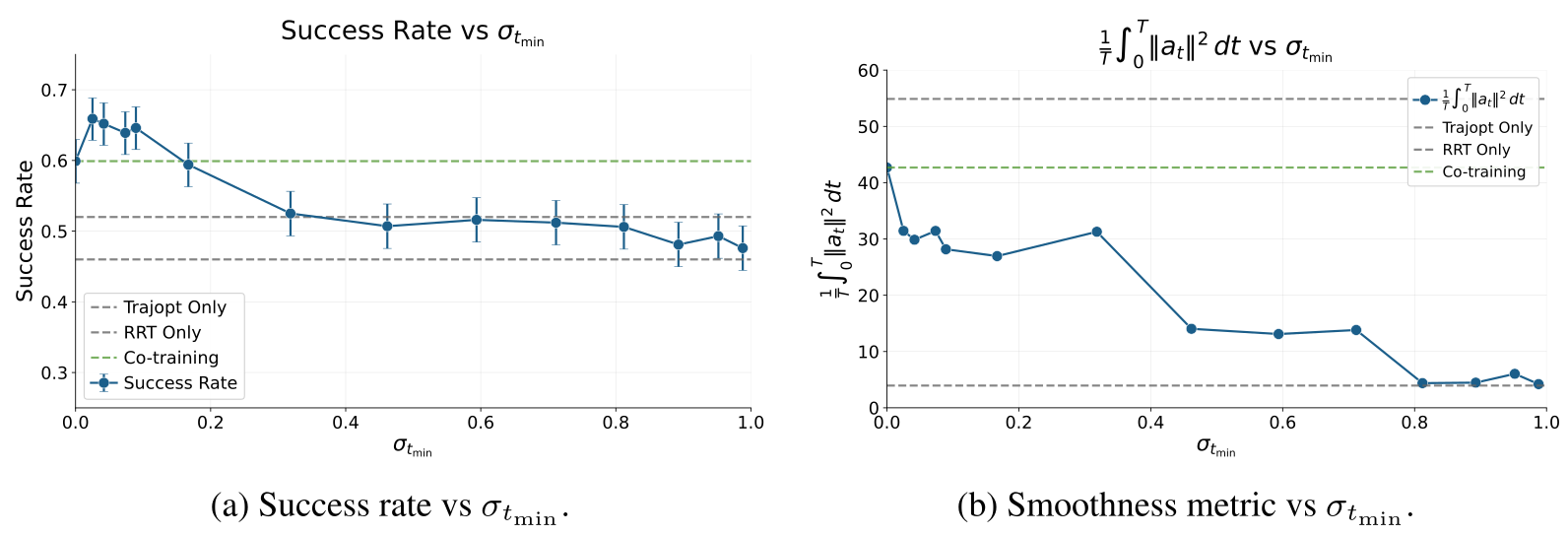
Selectable original panel labels
(a) Success rate vs .
(b) Smoothness metric vs .
G.3 Sim-and-Real Co-training: Planar Pushing
Both source and target are simulators. Their differences include lighting/colors/camera/shadows, quasistatic versus Drake physics and planner versus joystick actions. Success requires returning the pusher to its default position with the object within 1.5 cm and 3.5° of the goal in 75 seconds.
Eight ablations vary lower and upper cutoffs, classifier duration/threshold, Ambient-loss buffer, annotation granularity and auxiliary scale at two target-set sizes. Per-chunk labels perform best among the main variants; random chunk partitions with 10,000 groups are strongest in the partition study.
Sufficiently trained classifiers are relatively insensitive to checkpoint and threshold in this task. The optional loss is sensitive to its buffer. Auxiliary scaling generally favors Ambient, with an explicit exception at 4,000 auxiliary demonstrations and 50 target demonstrations. Locality does not help when the local contact dynamics differ.
| Gap | Simulation | Target Sim |
| Visual |
White spectrum light
Different object colors
Different camera pose
No shadows
|
Warm spectrum light
Different object colors
Different camera pose
Shadows
|
| Physics | Quasistatic | Drake physics [90] |
| Action | Motion planning | Human teleop |
Equation
Selectable original panel labels
(a) Performance vs (per dataset).
(b) Performance vs .
(c) Sensitivity to classifier training duration.
(d) Sensitivity to classifier threshold .
(e) Sensitivity to the Ambient loss buffer (Appendix C).
(f) Performance vs granularity of labels.
(g) Performance vs scale ().
(h) Performance vs scale ().
G.4 Task Mismatch: Block Sorting
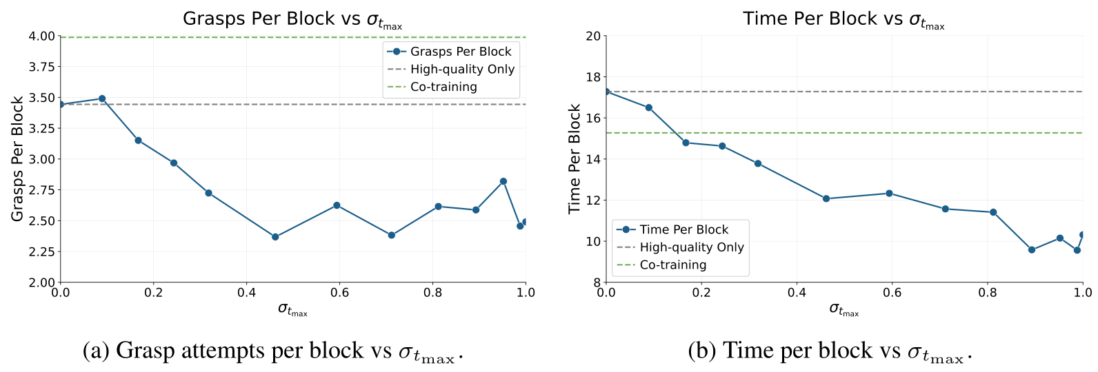
VR teleoperation collects both sorting datasets. Each of 200 trials contains one to three blocks of each color and allows twenty seconds per block, for roughly 800 evaluated blocks. Grasp attempts and time per block improve as the upper cutoff admits more low-noise practice.
With a one-hot task-direction input, co-training reaches 90.3% correct placements and Ambient 92.8%. A separate unconditioned policy using only wrong-task data at low noise still reaches 91.9%, with 97.9% conditional logic and 93.8% placement success. Task conditioning and time-dependent sampling are complementary here.
Selectable original panel labels
(a) Grasp attempts per block vs .
(b) Time per block vs .
| (a) Ablation 1: Task-Conditioned | (b) Ablation 2 | ||
| Training Algo. | Co-train | Locality | Locality |
| (# Blocks: 800) | () | () |
only below
|
| Logic | % | % | % |
| Motion | % | % | % |
| Success Rate | % | % | % |
Appendix H Scaling Experiments: Open X-Embodiment
The OXE appendix records curation, weighting, annotation, hardware evaluation and additional behavior measurements.
H.1 OXE Experiments
Custom OXE contains 48 accessible single-arm/mobile-manipulator datasets with compatible position/velocity actions, known frequency, proprioception and an RGB camera. It includes all 27 Magic Soup++ datasets and totals 1,402,606 demonstrations versus 1,279,774. This is an inclusive compatible subset, not all OXE data.
Weights reuse OpenVLA values where available; new-source weights mostly follow size with the two largest halved. Total target/auxiliary weight is .5/.5 before time-dependent normalization. Forty-eight binary classifiers label one lower cutoff per source; a single source-conditioned classifier is suggested but not used.
Upper cutoffs are fixed at diffusion step ten for cleaning and five for towers, without a sweep. A classifier-based upper-cutoff method would assign zero to nearly all sources, so the reported locality settings are manual choices.
Cleaning trains on 31 objects and evaluates three unseen objects per trial for ninety seconds. Opening/closing the drawer each earns .1 and each cleaned object .8/3. A bug supplies 128×128 inference images upscaled to 224×224, whereas training used 640×320 images resized to 224×224; all cleaning comparisons retain this mismatch.
Tower trials count correctly colored/oriented blocks until collapse or human intervention. Both tasks use twenty trials per policy; the camera bug was fixed for towers.
| Subtask | Points |
| Open drawer | 0.1 |
| Clean object (per object, 3 total) | |
| Close drawer (after table cleaned) | 0.1 |
| Max score per trial | 1.0 |
H.2 OXE Ablations
The additional OXE analysis examines repeated grasping and object-cleaning time, alongside the main weighting ablation and the finetuning appendix.
H.2.1 Qualitative Performance
Long cleaning timeouts can conceal repeated failed grasps. Across ten objects, Magic Soup++ Ambient reduces mean attempts from 2.4 to 1.6 and mean time from 24.9 to 14.8 seconds. Custom OXE reduces attempts from 2.1 to 1.7 and time from 22.1 to 16.1 seconds.
The tables report standard errors across ten per-object values. The custom-OXE attempt reduction is about 19%, smaller than the broad 25–40% prose claim; the exact object-level values remain visible.
| MS++ | COXE | |||
| Object | Co-train |
Ambient +
Locality
|
Co-train |
Ambient +
Locality
|
| Apple | 2 | 1 | 2 | 2 |
| Figurine | 4 | 2 | 2 | 2 |
| Eraser | 4 | 2 | 2 | 1 |
| Play-Doh | 2 | 2 | 2 | 2 |
| Robot Gripper | 3 | 2 | 2 | 2 |
| Yarn | 2 | 2 | 2 | 2 |
| Camera Mount | 1 | 1 | 1 | 2 |
| 3D Printed Object | 2 | 2 | 3 | 1 |
| Mustard | 3 | 1 | 2 | 2 |
| Garbage Bag Box | 1 | 1 | 3 | 1 |
| Average | ||||
| MS++ | COXE | |||
| Object | Co-train |
Ambient +
Locality
|
Co-train |
Ambient +
Locality
|
| Apple | 21s | 9s | 30s | 19s |
| Figurine | 44s | 20s | 30s | 20s |
| Eraser | 39s | 16s | 18s | 8s |
| Play-Doh | 20s | 20s | 19s | 20s |
| Robot Gripper | 31s | 19s | 19s | 20s |
| Yarn | 22s | 19s | 20s | 20s |
| Camera Mount | 12s | 8s | 8s | 20s |
| 3D Printed Object | 19s | 20s | 29s | 8s |
| Mustard | 33s | 9s | 18s | 19s |
| Garbage Bag Box | 8s | 8s | 30s | 7s |
| Average | s | s | s | s |
Appendix I Finetuning
Finetuning is evaluated as a complementary final stage, with explicit learning-rate reduction and checkpoint selection.
I.1 Implementation
Finetuning reduces learning rate ten- to twentyfold and saves checkpoints frequently because excessive updates can hurt. Simulation evaluates every checkpoint and reports the best; hardware screens checkpoints with five to ten trials before fully evaluating the selected one. Results therefore include selection effects.
I.2 Table Cleaning (OXE)
For fifty cleaning demonstrations plus custom OXE, Figure 23 shows approximately .71 for co-training before and after finetuning, and .83 to .82 for Ambient with locality. The paper reports no significant gain; this is not evidence of exact equivalence under every finetuning schedule.
Appendix J Distribution Shifts in the Observation Space
Action-distribution alignment does not directly address mismatched observations. The appendix explores two approaches without finding improvements in the tested cleaning setting; broader observation-shift handling remains open.
J.1 Noising the Observations
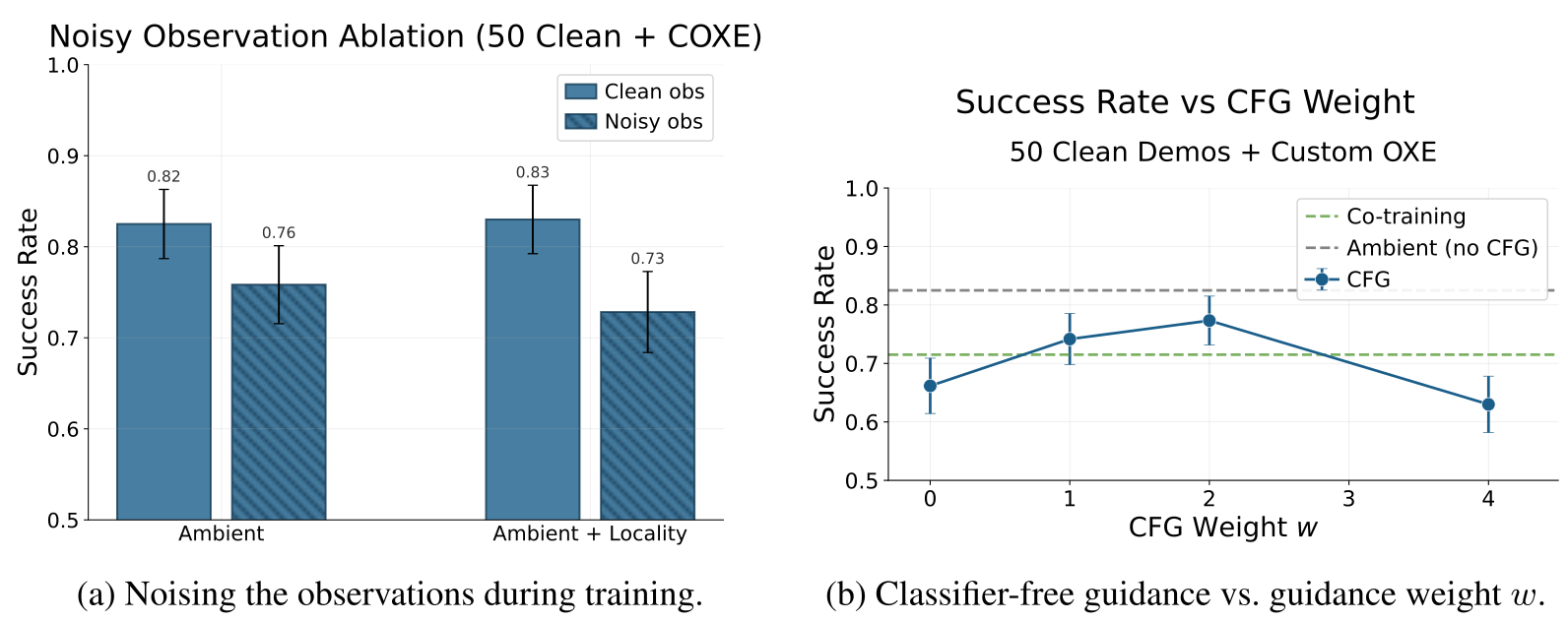
Half of training examples receive observation noise on the same schedule as action noise, with both noise levels supplied to the model. Inference uses clean observations. This did not improve table-cleaning performance; it differs in purpose from concurrent observation-noising work aimed at exploration for RL finetuning.
J.2 Classifier-Free Guidance
Classifier-free guidance trains conditional and observation-free denoisers, then extrapolates between their outputs with a guidance weight. Equation 87 retains the exact rule. Sweeping that weight did not improve the tested cleaning policy, so the presence of an unconditional branch did not solve the observed distribution shift.
Equation 87
| (87) |
Selectable original panel labels
(a) Noising the observations during training.
(b) Classifier-free guidance vs. guidance weight .