Overview
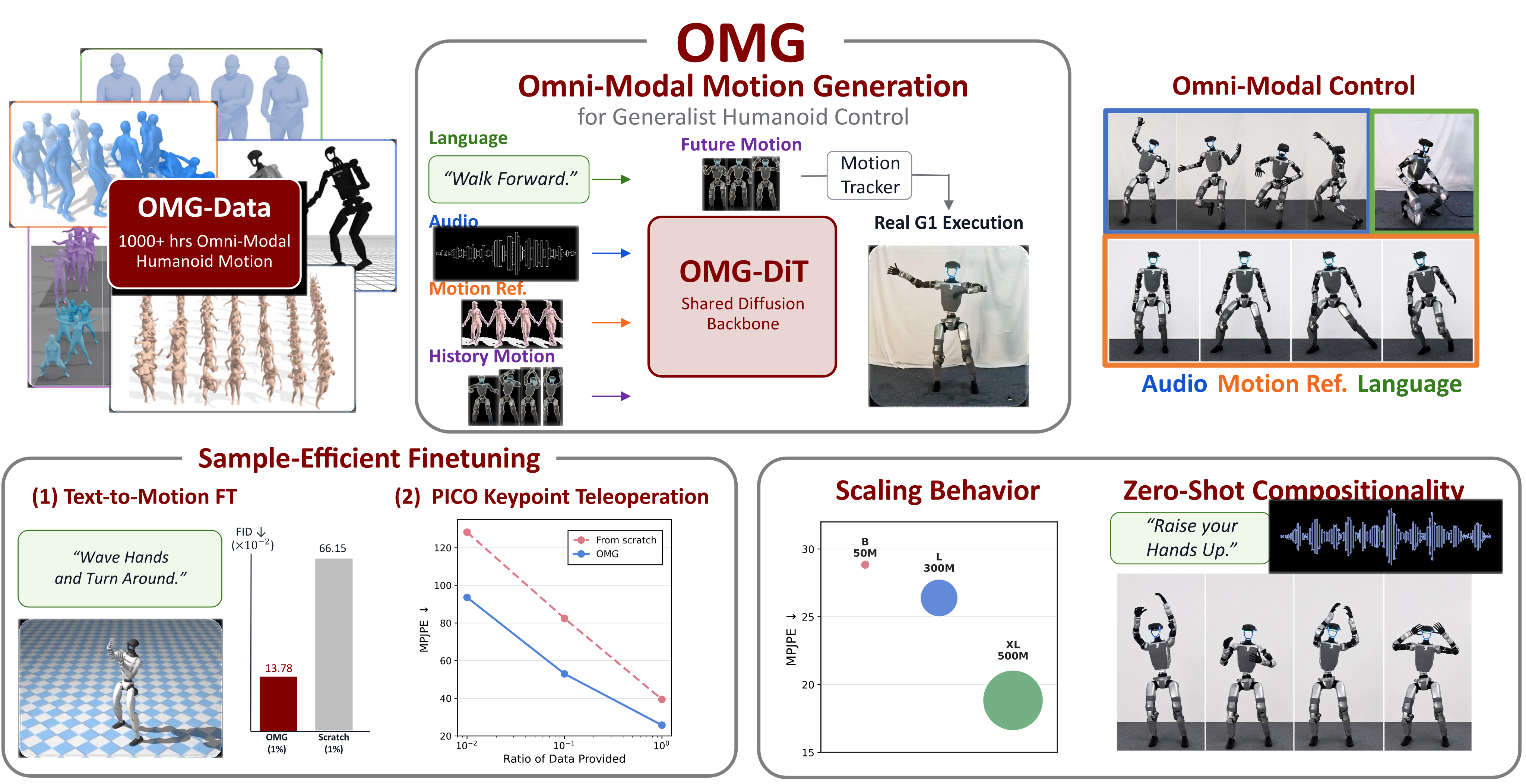
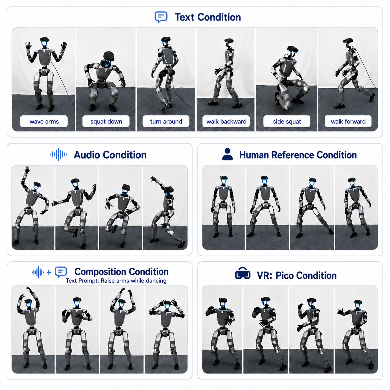
OMG generates future Unitree G1 motion from language, audio, human movement and combinations of these signals, then delegates execution to an existing tracker. The overview also introduces scaling and adaptation experiments.
At a glance
OMG combines a curated motion corpus with a diffusion transformer that predicts robot motion directly. Modality-specific encoders steer a shared motion prior, and a separate tracker executes generated trajectories. Results cover motion quality, execution fidelity, transfer to held-out motions and sparse-keypoint or visual interfaces, plus qualitative physical demonstrations. The evidence supports a reusable motion generator for this robot and data regime; it does not establish an unrestricted general-purpose humanoid controller.
1 Introduction
Motion tracking scales beyond individually engineered skills but still needs reference trajectories. OMG supplies those references from heterogeneous human commands. Its contributions are a G1-aligned multimodal corpus, a shared conditional diffusion backbone, and demonstrations of scaling, fine-tuning and compositional guidance. The generator–tracker hierarchy reuses HoloMotion for low-level execution; the new contribution lies mainly in the upstream motion prior and its conditioning interfaces.
2 Related Works
Related work separates the physical execution layer from the high-level generation layer that OMG aims to unify across modalities.
Humanoid Whole-Body Control and Motion Tracking.
Broad motion trackers follow many references but generally assume a motion or low-level command is already available. OMG builds on such a tracker rather than retraining the entire control hierarchy jointly.
Interactive and Multi-Modal Motion Generation.
Graphics models generate expressive human motion from text, audio or poses, often offline; previous robot generator–tracker systems usually support narrower inputs. OMG targets interactive multimodal generation directly in G1 space, reducing the inference-time need to retarget human output.
3 OMG-Data : Scaling Multi-Modal Data for Humanoid Motion Generation
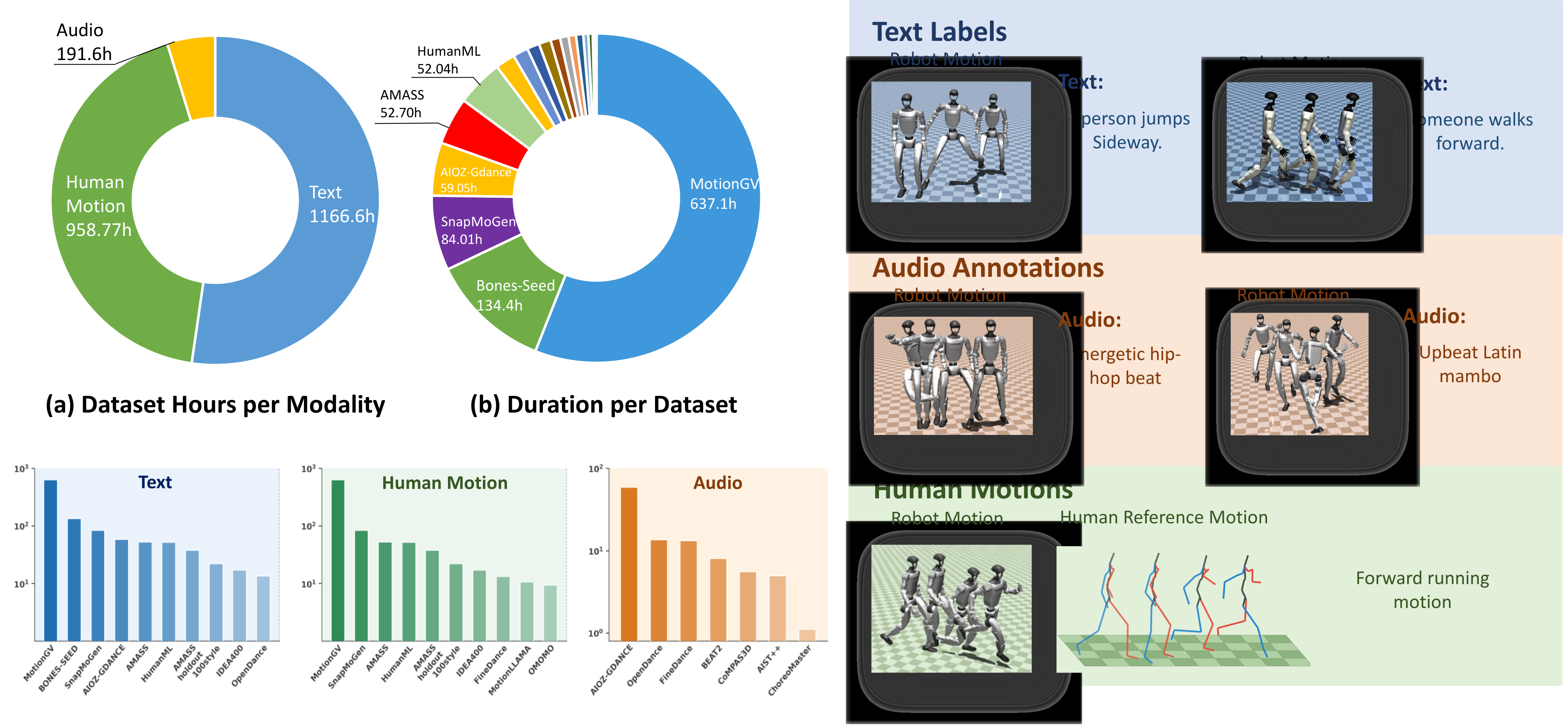
OMG-Data merges heterogeneous sources into G1 trajectories at 30 Hz. The reported 1,174.66-hour total includes the 38-hour CMU/Weizmann holdout row; the appendix states those subsets are excluded from pretraining. Summing the other processed-hour rows gives 1,136.66 hours. These reported dataset totals should therefore not be confused with the effective pretraining subset.
Data Curation and Preprocessing.
Corrupted files, broken links, severe frame gaps and invalid joints are removed. Audio waveforms and features are synchronized to motion frames so temporally aligned conditioning can be learned across dance and gesture datasets.
Motion Retargeting and Annotation.
GMR retargets heterogeneous skeletons into G1 space. Seed-1.8 labels rendered views or keyframes where language is absent or insufficiently granular. Training clips follow language boundaries, audio phrases or fixed sliding windows.
Simulation-In-The-Loop Filtering.
Motions are executed through the tracker in MuJoCo and rejected for persistent low root height or excessive tilt. The appendix also rejects non-finite states and, for stricter subsets, joint-limit violations. This screens feasibility under the chosen tracker and simulator; it is not a guarantee of collision freedom or safe physical deployment.
4 OMG-DiT : Unified Diffusion Backbone for Motion Generation
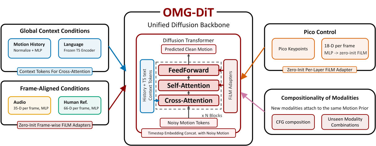
A shared denoising model learns the motion distribution while separate encoders translate commands into conditioning signals. This separates reuse of the motion prior from extension of the input interface.
4.1 Problem Formulation
The high-level policy predicts future reference states from conditions and recent motion history. The low-level HoloMotion policy maps those references and observed state into actions. OMG trains the generator and reuses the tracker, so generation and execution errors are evaluated separately.
Equation
4.2 Diffusion Transformer Backbone
The generator denoises motion features directly, with no learned motion tokenizer or latent autoencoder.
Motion Representation.
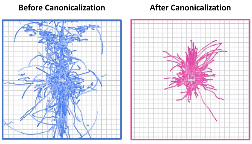
Each frame contains 125 features: local root position and 6D orientation, 29 joint angles, and 29 non-root body-link positions. Anchoring translation and heading at the last observed state removes arbitrary world placement while retaining local whole-body motion.
Model Architecture.
A diffusion transformer predicts clean motion. Recent motion enters through cross-attention; timestep features are concatenated with noisy input features. Global and frame-aligned command streams use different conditioning paths.
Training Objective.
Gaussian noise corrupts the future segment; squared-error training reconstructs its clean features. Independently dropping available modalities teaches conditional and null branches for classifier-free guidance and allows one model to use partially labelled datasets.
Equations 1–2
| (1) |
| (2) |
4.3 Omni-Modal Condition Encoding
Language supplies global context, whereas audio and human movement provide frame-aligned conditions.
Pretraining Condition Encoders.
Frozen T5 language features join motion-history tokens in cross-attention. Audio and human-reference features pass through MLPs and modulate corresponding future frames with FiLM at each transformer layer.
Task-specific Finetuning Encoders.
New interfaces use lightweight encoders and initially zero-output adapters, such as 18D Pico keypoints for teleoperation. The appendix clarifies that the reported adaptation experiments fine-tune all backbone parameters, rather than demonstrating encoder-only training.
5 Experiments
Experiments test pretrained generation, transfer versus matched training from scratch, and qualitative command composition and model-size scaling. A separate appendix evaluates a small visual locomotion task.
5.1 Experiment Setup
Generated G1 references are assessed both before and after tracker execution using held-out validation motions.
Evaluation Protocol.
Pretraining evaluation covers text, audio and human references. Adaptation covers unseen motion distributions and Pico keypoints, with the same architecture and data budgets for pretrained and scratch models. HoloMotion executes generated trajectories unless stated otherwise.
Metrics.
Generation metrics measure text alignment, distributional similarity, beat alignment or reference pose error. Execution metrics measure tracker deviation, sliding, jerk, falls and joint-limit violations. Stronger distributional scores need not imply better rhythm alignment or safer execution.
5.2 Pretraining Experiments
The three benchmark tables retain every generation, physical-quality and tracker-fidelity metric, including tradeoffs hidden by the broad claims in the prose.
| Methods | Motion Generation Quality | Tracking Fidelity and Execution Failures | ||||||||||||
|---|---|---|---|---|---|---|---|---|---|---|---|---|---|---|
| FID | Matching | R@1 | R@2 | R@3 | Diversity | C-Slide | Jerk | MPJPE | g-MPJPE | E_vel | E_acc | Fall | J-Limit | |
| GENMO | 43.78 | 1.33 | 12.99 | 23.83 | 30.86 | 1.28 | 2.66 | 173.54 | 50.35 | 150.71 | 6.91 | 2.51 | 1.46 | 29.10 |
| HYMotion | 24.68 | 1.30 | 31.84 | 48.73 | 57.71 | 1.29 | 12.20 | 112.56 | 69.05 | 287.71 | 11.94 | 3.24 | 4.98 | 55.57 |
| Kimodo-SMPLX-RP | 38.44 | 1.31 | 26.27 | 39.36 | 46.48 | 1.25 | 4.52 | 189.39 | 43.51 | 198.96 | 7.80 | 2.64 | 2.64 | 23.63 |
| Kimodo-G1-RP | 46.36 | 1.32 | 25.59 | 36.13 | 44.63 | 1.21 | 3.92 | 81.44 | 37.25 | 125.04 | 5.72 | 1.68 | 1.46 | 19.14 |
| Kimodo-G1-SEED | 50.22 | 1.33 | 22.46 | 33.69 | 41.11 | 1.20 | 4.30 | 99.47 | 37.26 | 161.63 | 6.38 | 1.84 | 1.56 | 20.70 |
| OMG-L | 9.55 | 1.14 | 58.50 | 74.90 | 81.45 | 1.39 | 3.68 | 56.03 | 39.06 | 98.37 | 5.11 | 1.47 | 0.29 | 14.94 |
| OMG-XL | 6.03 | 1.11 | 65.43 | 80.37 | 86.91 | 1.39 | 3.98 | 52.31 | 42.68 | 111.41 | 5.48 | 1.53 | 0.78 | 19.34 |
| Methods | Audio Alignment and Target Motion Quality | Target Physical Quality and Tracker Fidelity | ||||||||||
|---|---|---|---|---|---|---|---|---|---|---|---|---|
| BeatAlign | FIDk | FIDg | PFC | C-Slide | Jerk | MPJPE | g-MPJPE | E_vel | E_acc | Fall | J-Limit | |
| GENMO | 0.57 | 506.07 | 9.42 | 0.02 | 0.03 | 72.56 | 35.73 | 111.69 | 3.87 | 1.22 | 0.39 | 12.50 |
| LODGE | 0.58 | 390.06 | 11.98 | 1.41 | 0.65 | 471.45 | 149.19 | 363.24 | 18.89 | 6.96 | 39.45 | 66.80 |
| Bailando | 0.56 | 134.90 | 15.71 | 0.39 | 0.25 | 117.45 | 38.30 | 106.39 | 5.55 | 1.99 | 0.00 | 1.76 |
| OMG-L | 0.49 | 59.20 | 0.74 | 0.57 | 0.41 | 95.73 | 41.07 | 95.10 | 6.10 | 1.90 | 0.00 | 14.26 |
| OMG-XL | 0.51 | 40.46 | 0.63 | 0.64 | 0.43 | 106.06 | 41.47 | 97.60 | 6.03 | 1.94 | 0.00 | 15.43 |
| Methods | Target Motion and Physical Quality | Tracker-Executed Target Fidelity and Failures | |||||||||||
|---|---|---|---|---|---|---|---|---|---|---|---|---|---|
| MPJPE | g-MPJPE | EE Error | E_vel | E_acc | C-Slide | Jerk | Target MPJPE | Target g-MPJPE | Target E_vel | Target E_acc | Fall | J-Limit | |
| GMR | 81.95 | 223.69 | 219.23 | 11.72 | 10.41 | 0.45 | 404.80 | 90.54 | 249.47 | 12.52 | 5.22 | 11.33 | 68.75 |
| NMR | 173.77 | 390.82 | 477.08 | 14.87 | 7.43 | 0.77 | 97.75 | 102.28 | 299.27 | 11.26 | 3.32 | 14.84 | 87.89 |
| PHC | 51.44 | 153.44 | 152.18 | 5.06 | 3.97 | 0.45 | 131.38 | 47.80 | 115.92 | 5.86 | 1.99 | 3.71 | 39.45 |
| OmniRetarget | 56.90 | 119.71 | 131.14 | 5.55 | 4.87 | 0.31 | 188.92 | 44.34 | 111.58 | 5.94 | 2.35 | 0.98 | 24.22 |
| OMG-L | 26.40 | 64.64 | 72.39 | 6.16 | 3.91 | 0.35 | 61.01 | 42.81 | 110.66 | 5.63 | 1.62 | 0.20 | 22.66 |
| OMG-XL | 18.84 | 47.83 | 52.26 | 5.03 | 3.69 | 0.32 | 64.04 | 43.07 | 112.60 | 5.55 | 1.63 | 0.39 | 23.05 |
Text to Motion.
OMG-XL achieves the best displayed text FID and retrieval scores: FID 6.03 in the table’s ×10⁻² scale and R@1 65.43%. OMG-L has lower fall and joint-limit rates than XL (0.29%/14.94% versus 0.78%/19.34%). GENMO has less contact sliding and some Kimodo variants lower tracker MPJPE, so generation-quality gains are not uniform physical-metric wins.
Audio to Motion.
OMG-XL has the lowest audio distribution distances, FID-k 40.46 and FID-g 0.63. However, its BeatAlign 0.51 is below GENMO 0.57, LODGE 0.58 and Bailando 0.56, contrary to the source’s blanket claim of superior audio alignment. OMG has zero reported falls here but higher joint-limit violation than Bailando (15.43% versus 1.76% for XL); the full table shows the tradeoff.
Human Reference to Motion.
With human-reference conditioning, OMG-XL reduces target MPJPE to 18.84 mm and global error to 47.83 mm, versus 51.44/153.44 for PHC and 56.90/119.71 for OmniRetarget. Tracker-executed errors are larger: XL reaches 43.07/112.60 mm, with 0.39% falls and 23.05% joint-limit violations. Better generated references therefore do not remove the execution bottleneck.
5.3 Finetuning Experiments
Fine-tuning comparisons hold the model size, selected data and split fixed, changing pretrained versus random initialization.
Few-shot Text-to-Motion Finetuning.
At 1% of held-out target slices, text-motion fine-tuning lowers FID from 0.6615 to 0.1378; full-data scratch reaches 0.1001. Thus the small-data model approaches, but does not match, full-data scratch on FID or retrieval. At 100% data, pretrained FID is 0.0827. The results establish useful transfer; “1% equals full data” would overstate the table.
Pico Keypoint-Based Teleoperation.
Pretraining improves all displayed Pico metrics at 1%, 10% and 100% target data. With full data, MPJPE falls from 39.42 to 25.73 mm and global MPJPE from 134.85 to 77.01 mm. This extends the prior to a new sparse-keypoint interface with additional supervised adaptation.
5.4 Analysis
The analysis studies composition and three model sizes rather than establishing a universal scaling law.
Zero-shot Compositionality.
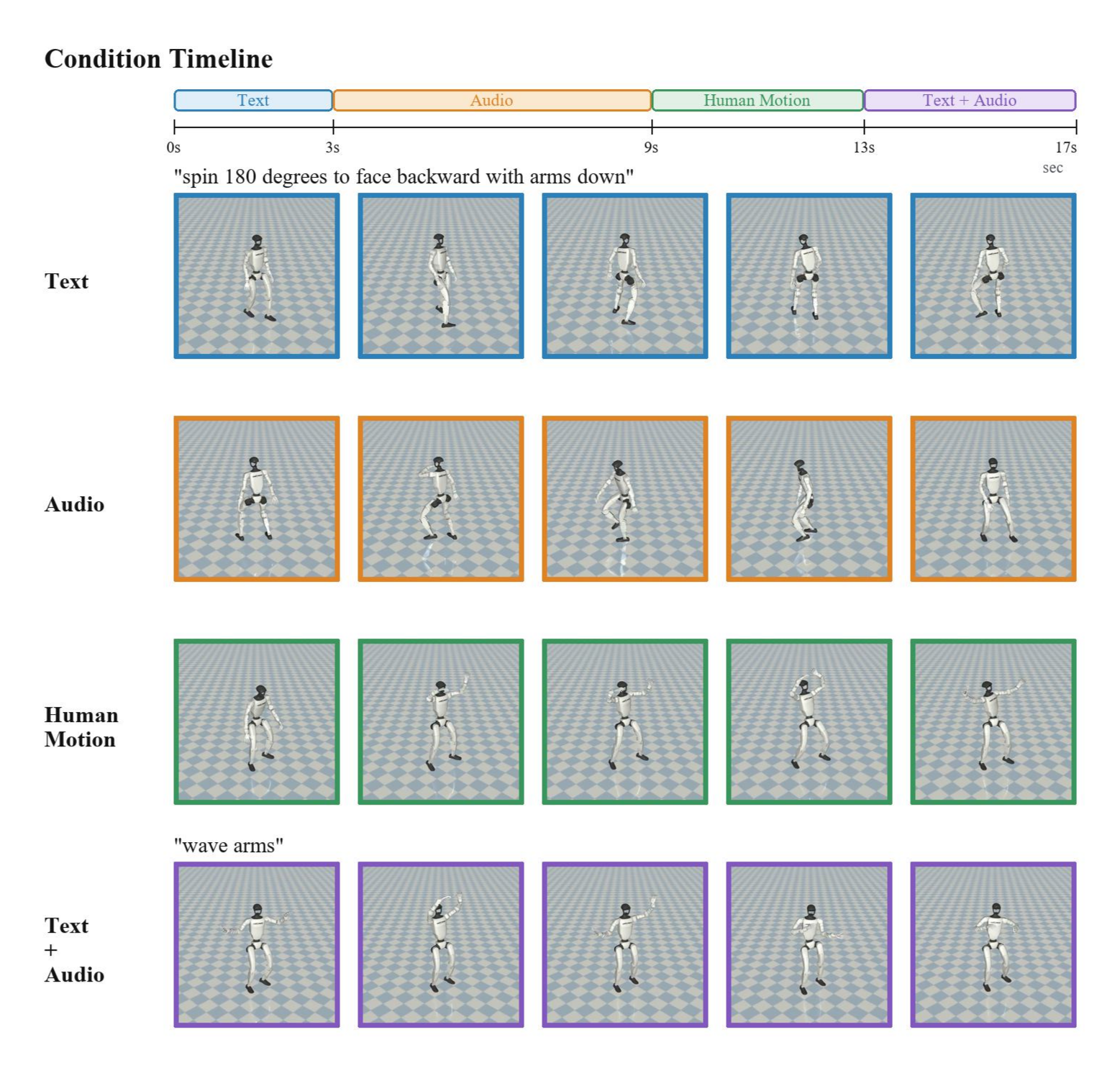
Separate text and audio guidance directions are combined at inference. Physical examples show raising or waving hands while following a music condition. These demonstrations illustrate unseen signal combinations qualitatively; no comprehensive compositional success-rate benchmark is reported.
Scaling Behavior.
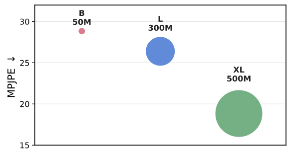
Increasing the backbone from 50M to 300M to 500M parameters improves the plotted human-reference MPJPE and several generation metrics. Some tracker metrics worsen from L to XL, so capacity improves the motion prior more consistently than execution fidelity. The study does not vary data scale independently or fit a predictive scaling law.
6 Conclusion
OMG shows that a shared motion prior can support several command types and transfer to new interfaces while using an existing tracker. Its strongest evidence is the benchmark and matched fine-tuning results; open-world generality remains beyond the reported experiments.
7 Limitations
Training mainly covers flat ground. Uneven terrain and in-the-wild conditions remain challenging, and the separately trained generator and tracker are not jointly optimized. Execution feedback or joint adaptation is proposed for future work. Simulator filtering and selected physical demonstrations do not resolve these limits.
Acknowledgments
The authors acknowledge discussions and feedback from Ziwen Zhuang, Zekun Qi, Haoyang Weng and Yue Chen.
Appendix A Extended Related Work
The extended context distinguishes low-level reusable behavior priors from the high-level multimodal interface studied here.
Behavior Foundation Models for Humanoid Robots.
Forward–backward and latent-conditioned behavior models support multiple execution objectives, while generative middleware can rewrite references for recovery. OMG instead concentrates on translating language, audio and human movement into robot references, complementing these low-level approaches.
Appendix B Details on OMG -Data
The data appendix specifies source composition, skeleton conversion, annotation, segmentation and simulator filtering. The complete original annotation prompt is preserved.
B.1 Dataset Composition
All sequences use 30 Hz. Table 6 lists original and processed samples, lengths, hours and available modalities. Its 1,174.66-hour total includes 38 hours of CMU/Weizmann held out from pretraining; MotionGV is the largest processed row at 637.14 hours. The total is a corpus accounting figure, not a claim that all listed rows were used to pretrain.
| Dataset | Label | Original | Processed | ||||
| # Samples | Avg. Length | Total Hours | # Samples | Avg. Length | Total Hours | ||
| AMASS [33] | , | 17.9K | 1.4K | 94.8 | 51.1K | 111 | 52.7 |
| AMASS (holdout CMU & WEIZMANN) [33] | , | 13.65K | 1.4K | 44.9 | 39.0K | 105 | 38 |
| LAFAN1 [10] | 40 | 6.6K | 2.5 | 977 | 240 | 2.2 | |
| OMOMO [16] | , | 5.9K | 179 | 10 | 15K | 67 | 9.4 |
| 100style [34] | , | 0.8K | 2.9K | 22.12 | 10.7K | 223 | 22.10 |
| HumanML [8] | , | 26.8K | 219 | 54.5 | 25.7K | 218 | 52.04 |
| Kungfu [8] | 1.0K | 453 | 4.3 | – | – | – | |
| MotionGV [8] | , | 56K | 140 | 727 | 53.8K | 128 | 637.14 |
| fitness [8] | , | 262 | 610 | 1.48 | 337 | 244 | 0.76 |
| MotionLLAMA (subset) [8] | , | 4.5K | 286 | 12 | 4.9K | 236 | 10.7 |
| SnapMoGen [9] | , | 50K | 407 | 188.7 | 41.0K | 222 | 84.01 |
| FineDance [19] | , , | 0.2K | 4.0K | 14.6 | 6.0K | 240 | 13.26 |
| BEAT2 [27] | , | 1.7K | 3.4K | 60 | 417 | 2.0K | 8.06 |
| AIST++ [20] | , , | 1.4K | 400 | 5.2 | 2.2K | 240 | 4.98 |
| IDEA400 [69, 25] | , | 12.5K | 176 | 20 | 10K | 177 | 17.24 |
| PerMo [14] | , | 6.6K | 140 | 8.6 | 6.5K | 139 | 8.38 |
| BONES-SEED [42] | 71K | 219 | 144 | 79K | 182 | 134.35 | |
| ChoreoMaster [3] | , | 2.7K | 46.7 | 1.2 | 2.5K | 47 | 1.11 |
| CoMPAS3D [2] | , | 4.8K | 138 | 6.2 | 4.66K | 129 | 5.57 |
| AIOZ-GDANCE [15] | , | 6K | 1.1K | 60.8 | 5.8K | 1091 | 59.05 |
| OpenDance [66] | , | 5.0K | 300 | 14.0 | 4.9K | 300 | 13.61 |
| Total | , , | 288.8K | 411 | 1496.9 | 364.5K | 177 | 1174.66 |
B.2 Details on Retargeting
SMPL/SMPL-X bodies are geometrically retargeted with GMR. Video-derived motions first use GENMO to recover human meshes. FBX skeletons use standardized joint mapping or GMR depending on their structure.
B.3 Details on Labeling
Seed-1.8 annotates changes in atomic action or motion style as consecutive, non-overlapping segments. The original prompt requires English style/action labels, action descriptions of at most 25 words, timestamps to one decimal place and a structured JSON response. Its full wording and indented example are retained below.
You are a humanoid robot motion labeling model (VLM). Your task is to perform structured motion labeling for the input video, rather than generating descriptive text.

[Most Important Rule]
You must segment when there is a change in "motion atomic action". If the specific action changes, even if the overall style remains consistent, you still need to create a new segment.

[Core Requirement]
Please divide the input video into multiple consecutive time segments, and generate a structured action label for each segment.

The output of each segment must include:
1. start time
2. end time
3. style
4. action

[Segmentation Criteria]
You should decide whether to split mainly based on:
- whether the motion style changes
- whether a finer motion style / type can be judged to have changed
- whether the main action changes

If the motion remains continuous and no obvious change occurs, do not over-segment.

[Action Requirements]
1. action must be written in English
2. action should summarize the concrete motion performed in this segment
3. action should describe the motion itself as much as possible, and should not write overly abstract content
4. action should be concise, and no more than 25 words
5. action should be helpful for training a text-to-motion generation model

[Style Requirements]
1. style must be written in English
2. style should summarize the motion style of this segment, such as smooth, intense, rhythmic, explosive, etc.
3. style should be concise

[Output Format]
Please output in JSON format:
{
  "video_summary": "overall summary of the video",
  "segments": [
    {
      "start_time": 0.0,
      "end_time": 1.5,
      "style": "smooth",
      "action": "raise both arms and step slowly to the left"
    },
    {
      "start_time": 1.5,
      "end_time": 3.0,
      "style": "rhythmic",
      "action": "turn torso and swing arms in alternating beats"
    }
  ]
}

[Output Constraints]
1. Output valid JSON only
2. Do not output any explanatory text
3. Time must be in seconds
4. Keep all start_time and end_time values to one decimal place
5. Segments must be consecutive and non-overlapping
6. start_time must be less than end_time
7. video_summary should be a brief summary of the whole video

[Goal]
Your output should help train a motion generation model, so the labels should preserve motion content, motion style, and temporal changes as much as possible.
B.4 Segmentation Details
Text clips follow annotation boundaries; audio clips follow phrases or uniform windows. Long episodes are split with sliding windows. Thus data-fraction experiments later select motion slices rather than independent people or episodes.
B.5 Simulation-in-the-Loop Filtering Details
The deployment tracker produces actions clipped at 10.0, which become desired joint positions for a PD executor over ten simulation substeps per control step. Filtering examines executed trajectories, rejecting non-finite states and sustained fall conditions; stricter subsets also reject joint-limit violations. The appendix uses at least ten fall frames, whereas the main text says over ten. Retained training trajectories are tracker executions, not merely original kinematic references.
Equations 3–4
| (3) |
| (4) |
Appendix C Details of OMG-DiT
The model appendix specifies representation, denoising, conditioning, guidance, adaptation and deployment details needed to interpret the experiments.
C.1 Motion Representation and Canonicalization
Canonicalization and normalization make trajectories comparable across world positions while retaining the robot’s full pose.
Motion Representation.
The 125D representation decomposes as 3 root-position values, 6 rotation values, 29 joint angles and 87 non-root link coordinates. Generation occurs directly in this feature space without a learned latent code.
Equation 5
| (5) |
Root Rotation Parameterization.
The first two rotation-matrix columns form a continuous 6D representation; orthonormalization recovers a valid orientation. This avoids quaternion sign ambiguity and output normalization constraints and was empirically more stable than the other parameterizations considered.
Canonicalization.
A ten-frame history predicts sixty future frames at 30 Hz. The last history root defines the anchor; subtracting its position and undoing its yaw canonicalizes root and link trajectories. Outputs are transformed back with the current anchor. Figure 6 illustrates removal of arbitrary translation and heading, not elimination of meaningful motion diversity.
Equations 6–7
| (6) |
| (7) |
Normalization.
Each canonical feature is standardized with training-split mean and variance, with a minimum standard deviation for stability. Samples are denormalized before conversion back to world-frame G1 state.
Equation 8
| (8) |
C.2 Denoising Backbone
The denoiser predicts the normalized clean future segment from noisy motion, timestep, recent history and available commands.
Equation 9
| (9) |
Architecture.
Bidirectional temporal self-attention spans sixty future frames; cross-attention supplies history and global conditions, while aligned signals modulate frames. RoPE encodes time and sinusoidal embeddings encode diffusion steps. B/L/XL use 50M/300M/500M parameters, widths 512/1152/1536, depths 10/14/13 and 8/18/24 attention heads.
| Model | Params | Hidden Dim. | Layers | Heads |
|---|---|---|---|---|
| OMG-DiT-B | 50M | 512 | 10 | 8 |
| OMG-DiT-L | 300M | 1152 | 14 | 18 |
| OMG-DiT-XL | 500M | 1536 | 13 | 24 |
Denoising Objective and Sampling.
Training uses a cosine noise schedule and clean-sample prediction. Default inference applies deterministic DDIM with fifty denoising steps. Single-condition guidance defaults to 2.5, while composed inputs can use separate scales.
Equation 10
| (10) |
C.3 Omni-Modal Condition Encoders
History, language, audio and human-reference channels use shared interfaces but different input encoders and dropout rates.
Motion History.
A two-layer MLP maps normalized ten-frame history into context tokens, accessed by cross-attention in every denoising block.
Language.
Frozen T5-Base encodes at most fifty text tokens; a projection maps them to the backbone width. Language is dropped with probability 0.3 during training.
Audio.
Audio is converted to mono, peak normalized and analyzed with a hop matched to 30 Hz and a Hann window of at least 50 ms. Equation 13 concatenates 32 normalized log-frequency-band energies, RMS energy, zero-crossing rate, and the sum of spectral flux and centroid, yielding 35 components. Features are padded/trimmed with a validity mask, projected and injected through FiLM; dropout is 0.1.
Equations 11–13
| (11) |
| (12) |
| (13) |
Human Reference Motion.
Human references contain 22 three-dimensional joint positions (66D), projected into frame-wise FiLM conditions. Dropout is 0.5. Availability masks disable missing modalities so datasets with different label subsets can train the same generator.
C.4 Adapting to New Modalities
Global new inputs join the cross-attention context; aligned inputs use FiLM or adaptive-normalization adapters. Zero initialization preserves the pretrained function at the start. Despite describing a lightweight default interface, the reported experiments use full backbone fine-tuning. Parameter-efficient adaptation is suggested as a possibility, not established by these results.
C.5 Classifier-Free Guidance and Composition
Guidance adds weighted differences between condition-specific and null predictions, allowing separately learned command effects to be combined.
Classifier-Free Guidance and Multi-Modal Composition.
For text, audio and human motion, separate conditional branches share a null branch. Their weighted prediction differences are added to the null prediction. Modality dropout makes these branches available; this additive composition does not guarantee compatibility for arbitrary conflicting commands.
Equation 14
| (14) |
Practical Implementation.
A single global scale compares a full-condition branch with null; separate scales instead combine separate modality branches. Defaults are 2.5 for a global scale, text/audio 3.0/1.5 for composition, and human-reference 2.0. Increasing a scale biases generation toward that signal but can hurt other metrics.
Equation 15
| (15) |
Extending Classifier-Free Guidance to New Modalities.
A new modality receives its own conditional-minus-null guidance direction, which can be combined with existing signals after adaptation.
Equation 16
| (16) |
C.6 Real-Time Deployment
Deployment runs the tracker onboard NVIDIA Orin and the generator offboard on an RTX 4090 linked by wired Ethernet. ONNX/TensorRT, FP16 and denoising caching reduce computation. This is a networked generator–tracker deployment, not evidence that the full generator runs onboard.
C.7 Training Hyperparameters
Pretraining uses AdamW at 6×10⁻⁵, weight decay 0.01, 2,000 warmup steps, cosine decay, gradient norm clipping at 1.0 and mixed bfloat16. Table 8 gives a maximum 100,000 steps and global batch 1,024 across eight A800 GPUs. The authors report completion in under ten hours; these settings describe this training run rather than a measured scaling study.
| Hyperparameter | Value |
| Motion Setup | |
| Prediction / history length | 60 / 10 frames |
| Motion frame rate | 30 FPS |
| Motion representation | 125D G1 features with 6D root rotation |
| Optimization | |
| Optimizer | AdamW |
| Learning rate | |
| Weight decay | |
| LR schedule | Linear warmup, cosine decay |
| Warmup steps | |
| Minimum LR | |
| Gradient clipping | Global norm |
| Training | |
| Max training steps | |
| Precision | bf16 mixed precision |
| GPUs | 8 |
| Per-GPU batch size | 128 |
| Global batch size | 1,024 |
| Inference | |
| Method | DDIM |
| NFE calls | 50 |
Appendix D Experiment Details
The evaluation appendix standardizes robot output format, splits, metrics, evaluator training and baseline conversions.
D.1 Evaluation Protocols
All task comparisons ultimately use G1 outputs and a shared evaluation pipeline, including baselines that originally generate human skeletons.
D.1.1 Evaluated Tasks and Motion Format
The common representation separates stored robot configuration from the richer features used by the generator.
Evaluated Tasks.
Six tasks are evaluated: text, audio and human-reference generation, Pico teleoperation, held-out text-motion fine-tuning, and visual locomotion.
Motion Format.
Stored G1 qpos has 36 values: 3 root positions, 4 quaternion components and 29 joint angles. Forward kinematics yields 90 coordinates for thirty body points. Non-G1 baseline outputs are converted or retargeted before this shared evaluation.
Equations 17–18
| (17) |
| (18) |
D.1.2 Evaluation Data Settings
Validation conditions are sampled separately from generator training; held-out subsets are reserved for adaptation comparisons.
Evaluation Data Split.
Text generation and text fine-tuning each use 1,024 validation conditions; audio, human-reference and Pico evaluations use 512. Default clips contain sixty frames. Text retrieval uses batches of 32 with dataset-stratified reordering, and FID references match sample count unless otherwise set. CMU and Weizmann are excluded from normal pretraining.
| Task | Evaluation data | # samples |
|---|---|---|
| Text-to-motion | Caption-bearing validation samples | 1024 |
| Audio-to-motion | Validation samples with audio/music features | 512 |
| Human reference-to-motion | Validation samples with human reference motion | 512 |
| Pico teleoperation | AMASS (CMU + WEIZMANN), with Pico keypoints | 512 |
| Text-to-motion finetuning | AMASS (CMU + WEIZMANN), with captions | 1024 |
D.2 Evaluation Metrics
Metrics distinguish target similarity, distributional quality, physical plausibility and actual tracker failures; no single score measures all of them.
D.2.1 Shared Evaluation Metrics
MPJPE compares root-relative body positions; global MPJPE retains translation. Velocity and acceleration errors use frame differences, whereas jerk and contact sliding include frame-rate factors. Fall and joint-limit rates are sequence-level indicators; a limit violation above 10⁻⁴ anywhere in a sequence counts. Original formulas and units remain in Table 10.
Equation 19
| (19) |
| Metric | Formula | Description |
|---|---|---|
| c-slide | Horizontal foot sliding speed during contact | |
| Jerk | Third-order motion variation | |
| g-MPJPE | Global body position error in mm | |
| MPJPE | Root-relative body position error in mm | |
| e-vel | Velocity error in mm/frame | |
| e-acc | Acceleration error in mm/frame2 | |
| Fall Rate | Sequence-level fall rate | |
| J-Limit | Sequence-level joint-limit violation rate |
D.2.2 Text-to-Motion Metrics
A separately learned embedding space supplies text-motion distance, within-batch top-K retrieval, Gaussian Fréchet distance and pairwise diversity. Diversity uses 300 random pairs by default. These are evaluator-dependent proxies for semantic and distributional quality, not direct physical execution measures.
| Metric | Formula | Description |
|---|---|---|
| Matching Score | Average distance between paired text-motion embeddings | |
| R-precision@K | Whether the ground-truth text is in the top- retrieval results | |
| FID | Fréchet distance between real and generated motion embeddings | |
| Diversity | Average embedding distance between generated samples |
Equation 20
| (20) |
D.2.3 Audio-to-Motion Metrics
Beat alignment scores the temporal distance between music and nearest motion beats, with Gaussian width 3/30 seconds. Kinetic and geometric FID compare motion statistics; PFC penalizes joint foot sliding during upward root acceleration. Their different targets explain why a method can improve FID while worsening rhythm alignment.
D.2.4 Details on Evaluator Training for Text-to-Motion Evaluation
A motion encoder and frozen T5-3B plus trainable projection learn a shared normalized embedding using symmetric InfoNCE. The motion encoder uses four transformer layers, eight heads and 512D features. Evaluation training uses the corresponding training split; adaptation evaluators are restricted to CMU/Weizmann. This encoder is an evaluation instrument, separate from the generator’s T5-Base conditioning encoder.
| Stage | Architecture | Output |
|---|---|---|
| Movement encoder | Linear + LayerNorm + GELU + Dropout | Per-frame feature |
| Hidden projection | Linear or Identity | Hidden sequence |
| Temporal encoder | RoPE Transformer | Temporal feature sequence |
| Pooling/projection | Mean pooling + MLP projection | Motion embedding |
| Normalization | L2 normalization | Unit-norm embedding |
| Hyperparameter | Value |
|---|---|
| Motion input dim | 90 |
| Movement dim | 512 |
| Hidden dim | 512 |
| Output dim | 512 |
| Transformer layers | 4 |
| Attention heads | 8 |
| MLP ratio | 4 |
Equations 21–23
| (21) |
| (22) |
| (23) |
D.3 Details of Evaluation Baselines
Baseline output spaces and conversion routes are explicitly retained, since retargeting can affect the final robot metrics.
D.3.1 Text-to-Motion Baselines
GENMO and HYMotion outputs pass through human-body conversion and GMR. Kimodo variants either generate SMPL-X for retargeting or produce G1 directly. The compared graphics generators produce full sequences in advance rather than the same interactive replanning interface.
| Baseline | Original output space | Conversion to G1 | Final artifact |
|---|---|---|---|
| GENMO [17] + GMR | SMPL-X motion | GMR retargeting | G1 qpos_36 |
| HYMotion [55] + GMR | SMPL/SMPL-H style motion | Convert to SMPL-X, then GMR | G1 qpos_36 |
| Kimodo-SMPLX-RP-v1 [42] + GMR | SMPL-X motion | GMR retargeting | G1 qpos_36 |
| Kimodo-G1-RP-v1 [42] | G1 qpos | Direct use | G1 qpos_36 |
| Kimodo-G1-SEED-v1 [42, 44] | G1 qpos | Direct use | G1 qpos_36 |
D.3.2 Audio-to-Motion Baselines
GENMO, LODGE and Bailando++ use their respective audio interfaces and human-motion formats, then convert through GMR to G1. The main table labels the last baseline Bailando while the appendix calls it Bailando++; both source labels are retained.
| Baseline | Condition input | Original output | Conversion to G1 | Final artifact |
|---|---|---|---|---|
| GENMO [17] + GMR | Raw audio/music embedding | SMPL-X motion | GMR retargeting | G1 qpos_36 |
| LODGE [18] + GMR | Music feature .npy | Dance motion array | Convert to SMPL/SMPL-X, then GMR | G1 qpos_36 |
| Bailando++ [46] + GMR | Raw audio/extracted feature | SMPL pickle | Convert to SMPL-X, then GMR | G1 qpos_36 |
D.3.3 Human Reference-to-Motion Baselines
GMR, PHC and OmniRetarget use geometric or physics-based retargeting, while NMR learns a mapping. All are compared after conversion to G1, with the same 22-joint human input interpretation.
Equation 24
| (24) |
| Baseline | Type | Intermediate representation | Final artifact |
|---|---|---|---|
| GMR [1] | Geometric/rule-based retargeting | Compact SMPL-X motion | G1 qpos_36 |
| PHC [31] | Physics/fitting-based retargeting | AMASS-style SMPL motion | G1 qpos_36 |
| OmniRetarget [59] | Optimization-based retargeting | Holosoma-compatible SMPL-X motion | G1 qpos_36 |
| NMR [72] | Learned retargeting model | Standard SMPL-X motion | G1 qpos_36 |
D.4 Details on Finetuning and Scaling Experiments
Fine-tuning fractions and model-size experiments control different variables and should not be conflated.
Datasets and Evaluation Splits.
Held-out annotated segments are exhaustively sliced into two-second windows, shuffled with a fixed seed, and truncated to the requested percentage. These percentages measure slices, not independent episodes. Scaling experiments reuse the same pretraining corpus.
Setup.
Adaptation compares the pretrained 300M L model with the same randomly initialized architecture. Parameter-scaling comparisons vary size while keeping the other settings fixed. The visual locomotion appendix adds a distinct adaptation test.
Appendix E Extended Experiments and Visualizations
Additional material contains timing measurements, physical qualitative sequences, temporal composition, guidance sweeps and visual locomotion adaptation.
E.1 Runtime Acceleration Analysis
For the 50M B model on one A800, sampling a two-second text-conditioned chunk falls from 1,297.9±12.5 ms in eager PyTorch to 51.7±1.5 ms with TensorRT, FP16 and caching (25.1×). The final denoiser time is 31.2 ms with 38 conditional/null predictions in nineteen backend calls. Timings average five steady-state runs and begin with cached condition tensors; they exclude the full sensing/network/control loop and do not directly measure the deployed RTX 4090 configuration.
| Optimization | Sampling (ms) | Denoiser infer (ms) | NFE (calls) | Speedup |
|---|---|---|---|---|
| PyTorch eager | 1297.9 12.5 | 1265.0 12.4 | 100 (100) | 1.0 |
| + torch.compile | 467.9 2.9 | 435.6 2.8 | 100 (100) | 2.8 |
| + ONNX Runtime CUDA | 358.2 24.2 | 337.0 22.7 | 100 (50) | 3.6 |
| + TensorRT engine | 127.3 7.3 | 100.9 4.3 | 100 (50) | 10.2 |
| + TensorRT FP16 | 99.8 5.2 | 73.3 5.2 | 100 (50) | 13.0 |
| + DiT cache | 51.7 1.5 | 31.2 1.3 | 38 (19) | 25.1 |
E.2 Extended Visualizations on Real-Time Omni-Modal Control
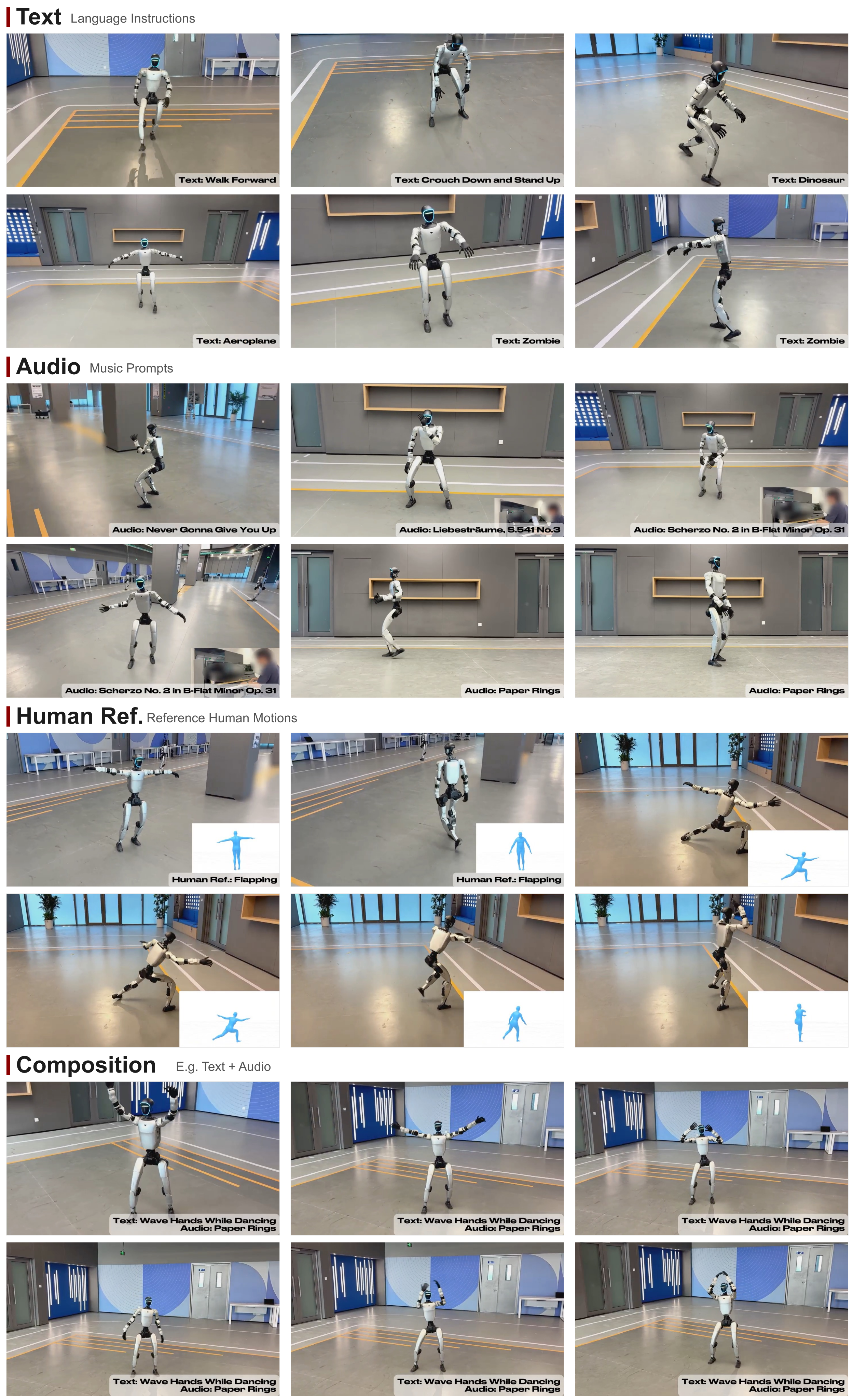
Figure 7 preserves the physical sequences and embedded commands for text, music, human motion and composed text/audio. These illustrate diversity and executability under selected conditions, without a trial-level success denominator.
E.3 Interactive Control with Temporal Composition
Figure 8 changes commands over time from text through audio and human reference to combined text/audio. The displayed rollout illustrates transitions while retaining local conditioning; smoothness and generality are assessed qualitatively here.
E.4 Analysis on Classifier-Free Guidance
Guidance sweeps examine alignment and the competing influence of command modalities. They show useful steering with metric-dependent tradeoffs.
Single-Modality Classifier-Free Guidance.
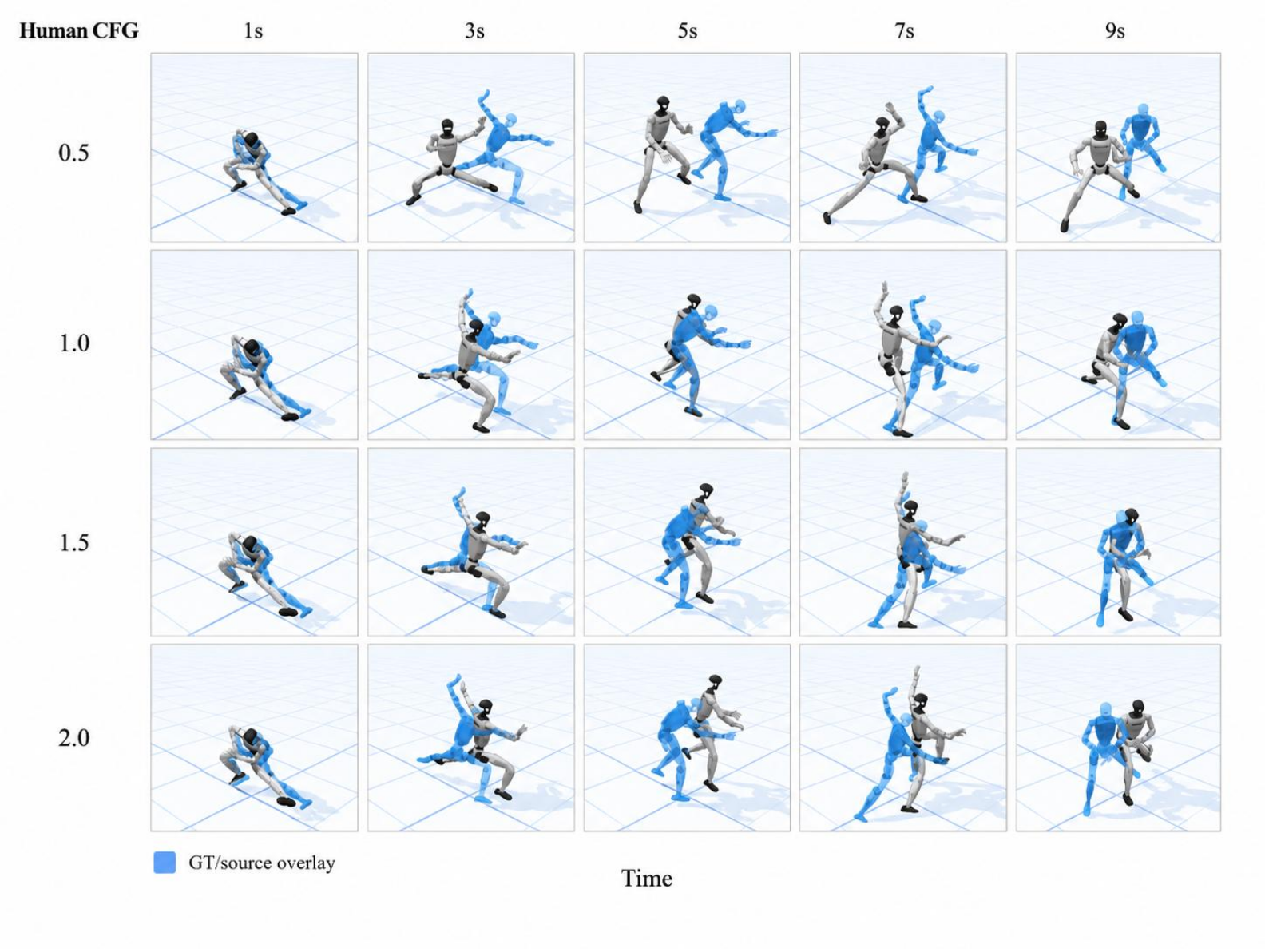
Increasing human guidance from 0.5 to 1.5 improves aggregate MPJPE/global MPJPE from 190.3/557.0 to 74.0/218.9 mm. At 2.0, MPJPE improves further to 71.0 but global error worsens to 343.9 mm; the time-specific columns are also non-monotone. Moderate guidance helps overall, but no single scale dominates every metric and horizon.
| Human CFG | MPJPE | g-MPJPE | 1s | 3s | 5s | 7s | 9s |
|---|---|---|---|---|---|---|---|
| 0.5 | 190.3 | 557.0 | 62.7 | 407.2 | 236.1 | 213.2 | 91.5 |
| 1.0 | 96.6 | 261.8 | 42.9 | 59.3 | 117.3 | 144.0 | 216.6 |
| 1.5 | 74.0 | 218.9 | 38.5 | 51.6 | 108.9 | 93.2 | 139.2 |
| 2.0 | 71.0 | 343.9 | 38.3 | 60.4 | 109.5 | 82.6 | 73.4 |
Multi-Modality Classifier-Free Guidance.
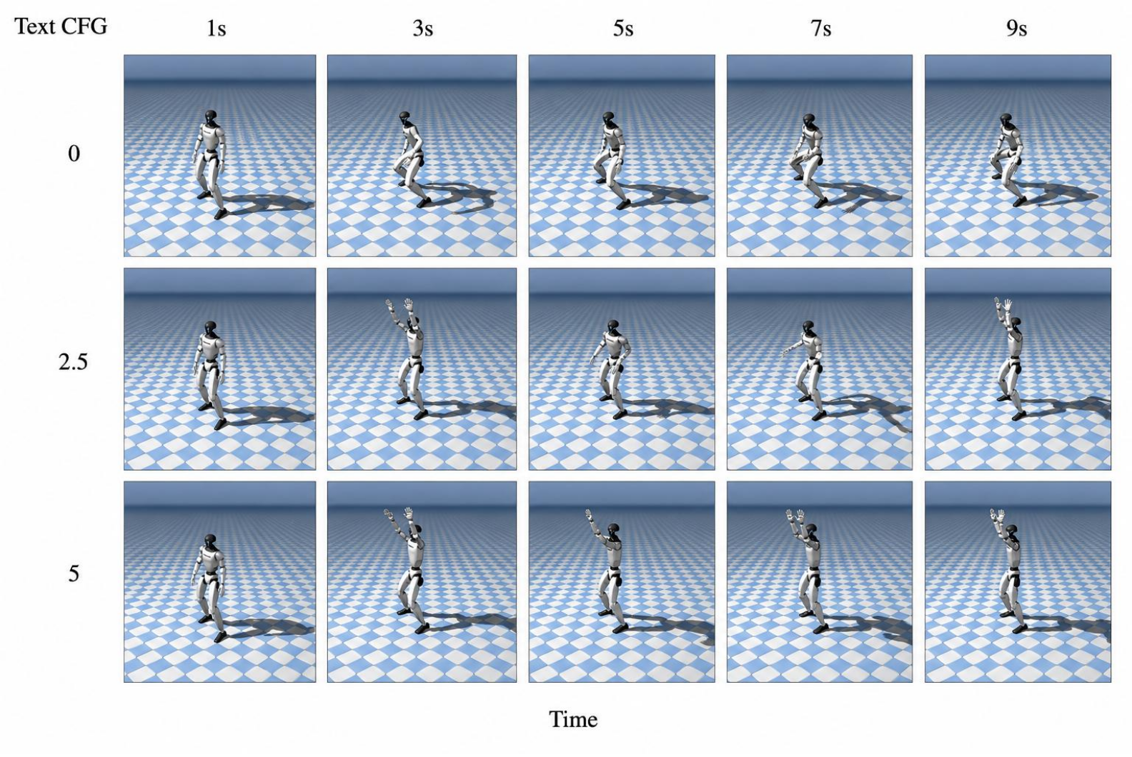
With a fixed music condition, stronger text guidance makes the robot raise its hands more clearly. The snapshots show semantic steering, while preservation of rhythm is qualitative rather than accompanied by a beat-score sweep.
E.5 Adaptation to New Modalities: Perceptive Locomotion
A small simulated visual task tests adaptation of the prior to an input modality absent from the original conditioning set.
Task and Environment.
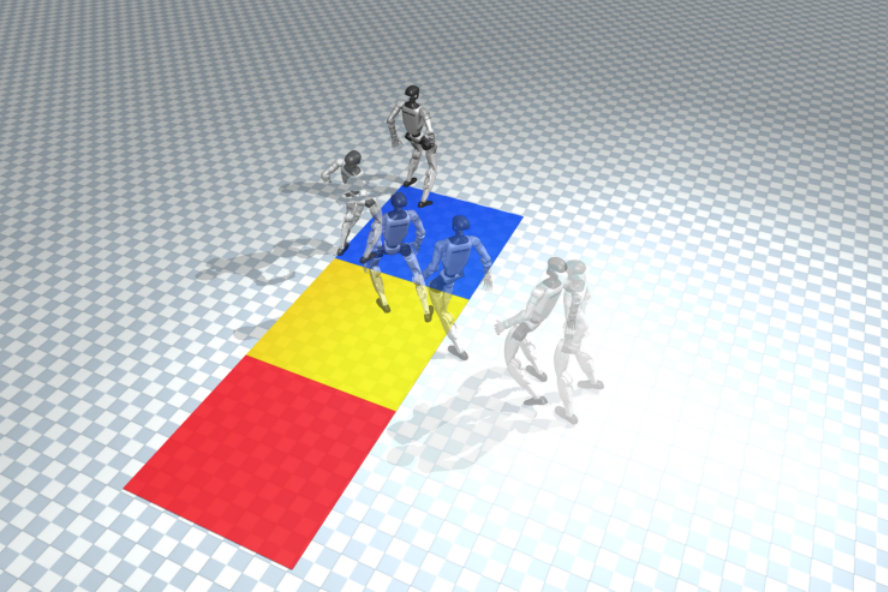
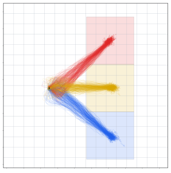
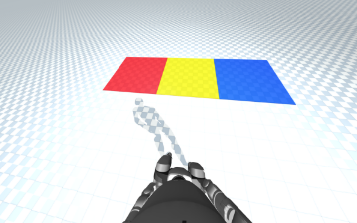
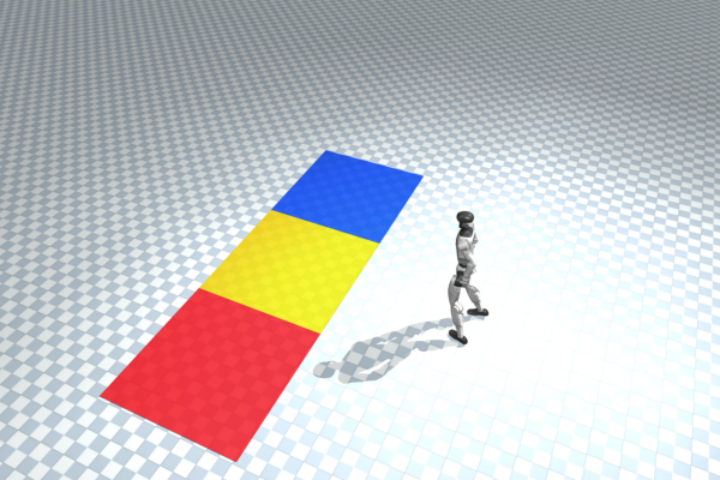
The robot sees an egocentric camera frame and a categorical instruction to reach one of three adjacent colored squares. This isolates simple visual grounding rather than general obstacle-aware navigation.
Training Data.
Kimodo generates 300 demonstrations per color, each with 210 frames and a terminal hold. Training samples two-second windows and a 64×64 RGB image. A learned yellow/blue/red embedding replaces language to keep the comparison controlled.
Model and Training Details.
Scratch and pretrained 300M models share the new RGB patch encoder, visual cross-attention and color embedding. A visual gate starts at 0.05, rather than zero. Both use one GPU, batch size sixteen and learning rate 6×10⁻⁵.
Evaluation and Results.
Replanning samples two seconds, executes the first half-second, and repeats for a 210-frame budget. Success requires the pelvis to enter the instructed square at any time, not remain there or meet a stopping criterion. After 500 updates, pretraining succeeds in 53/90 trials (58.9%) versus 44/90 (48.9%) from scratch: a ten-point improvement on this limited simulated task.
| Initialization | Step | Success Rate |
|---|---|---|
| Scratch | 500 | 44/90 (48.9%) |
| Pretrained | 500 | 53/90 (58.9%) |