At a glance
This edition follows the complete eight-page, 8 June 2026 v1, retaining all six figures and their panels, four tables, 27 numbered equations and 22 references.
Shared multi-agent policies learn to arrange mobile robots beneath an irregular object while avoiding obstacles and balancing an estimated load. Training combines local motion sensing with team positions/loads and a centralized critic. The simulation results favor load-aware formations over geometry-only baselines. The study concerns preparation for transport; lifting, carried-object dynamics and physical deployment are not evaluated.
I INTRODUCTION
Cooperative transport can use pushing, grasping, caging or support from below. Kiva-style systems rely on matched robot/object interfaces, while flexible support sheets add compliance and tension. This work instead asks robots to choose their own support positions beneath a rigid object with an irregular footprint and shifted center of mass.
The object is already suspended above the robots. The learned task is to enter its footprint and distribute an algebraic load estimate evenly; a balanced formation is a prerequisite for later transport, not evidence that the object has been lifted or carried safely.
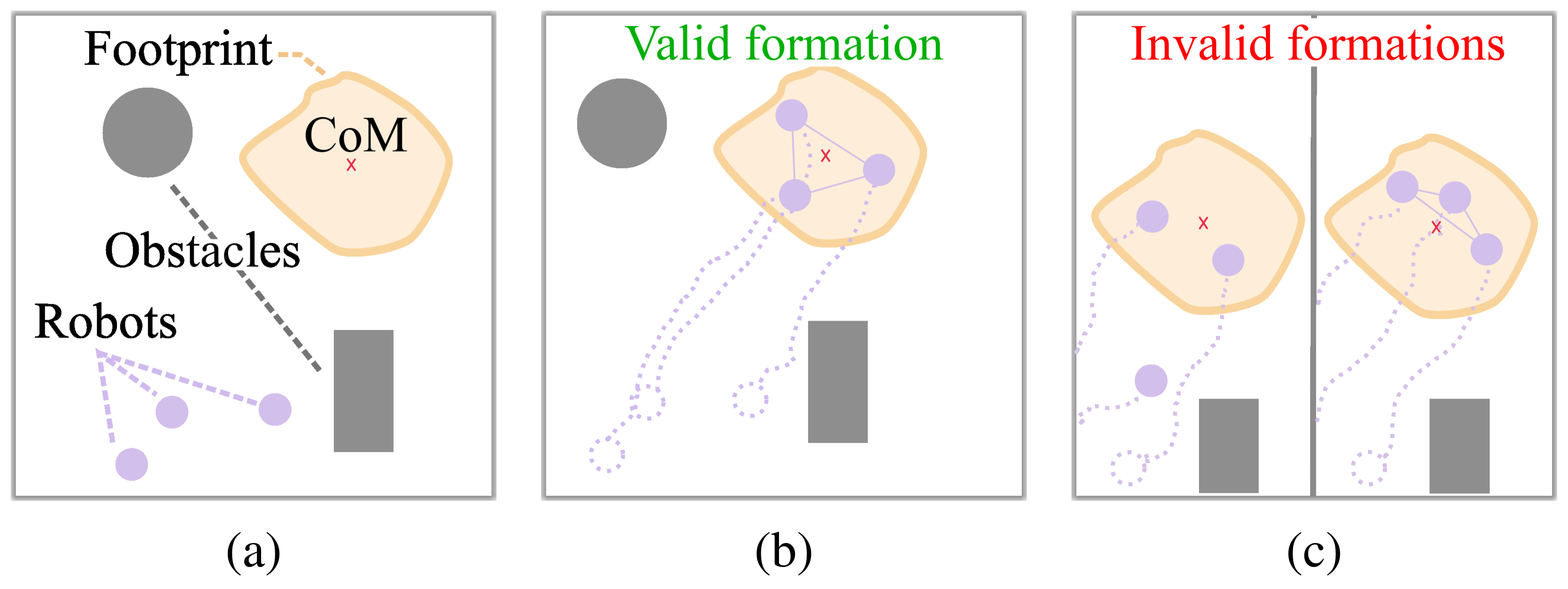
Original panel labels
II RELATED WORK
II-A Cooperative Object Transport
Prior transport controllers use hierarchical optimization, finite-state behaviors or decentralized negotiation, often with predefined attachment points or geometric formations. Pattern-formation methods fill or outline target shapes; image-moment control includes the center of mass but does not necessarily keep every robot inside the footprint. The proposed reward explicitly adds load balance rather than prescribing target positions.
II-B Multi-Agent Reinforcement Learning
Multi-agent reinforcement learning must address changing teammates, credit assignment and scaling. Centralized training with decentralized execution gives actors their own observation vectors while a critic sees the joint observations. Earlier Pattern-RL and swarm-learning methods target geometric arrangements; this work adds object-load information and omits fixed robot goal poses.
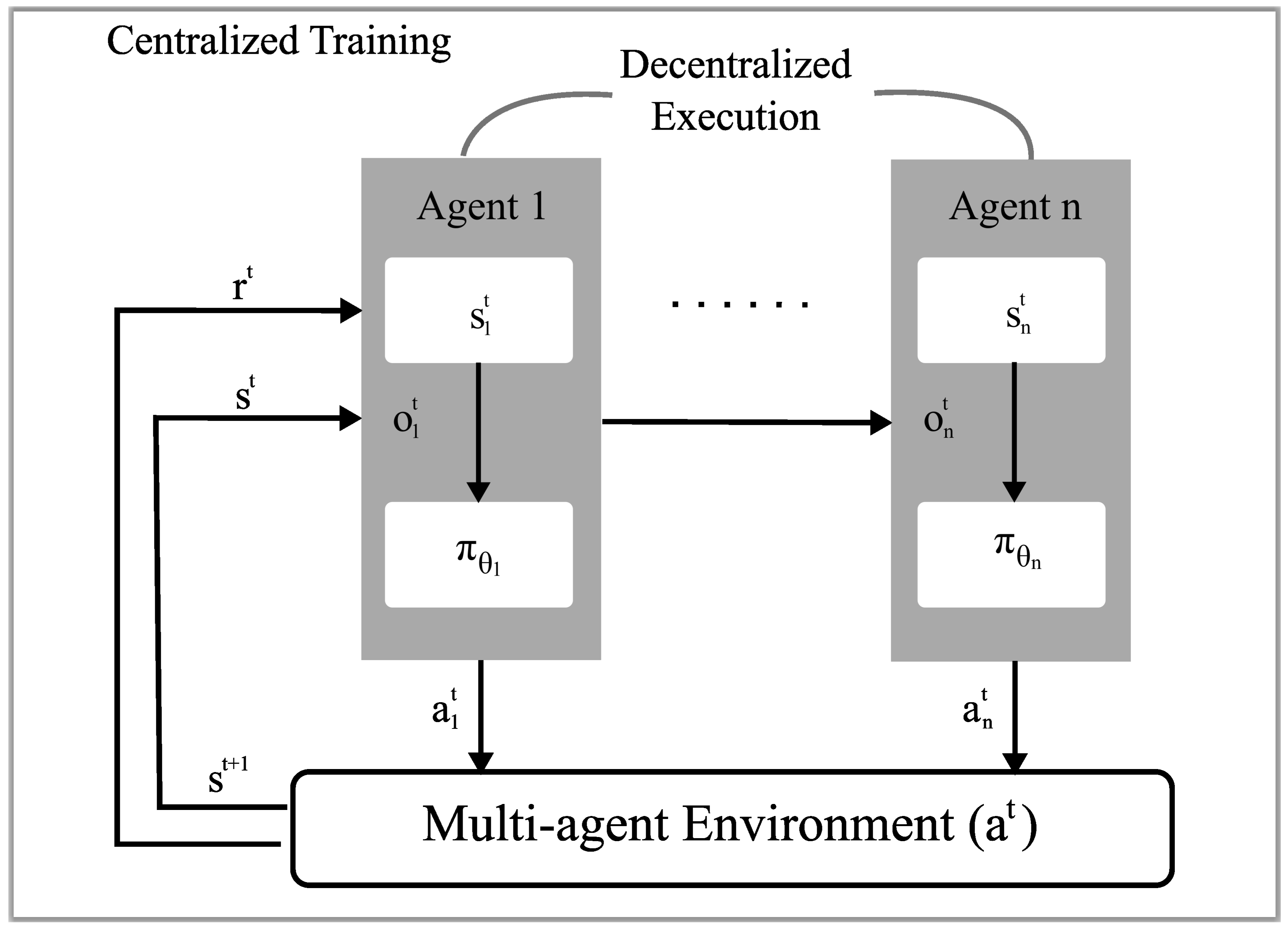
III METHODS
III-A Task Description
Circular mobile robots begin at random positions among static obstacles. The target is a suspended rigid object represented by a two-dimensional polygon; robots cannot collide with the object itself. Tests progress from uniform polygons to shifted centers of mass and footprints with cavities. Geometry and load information come from the simulator, rather than onboard estimation.
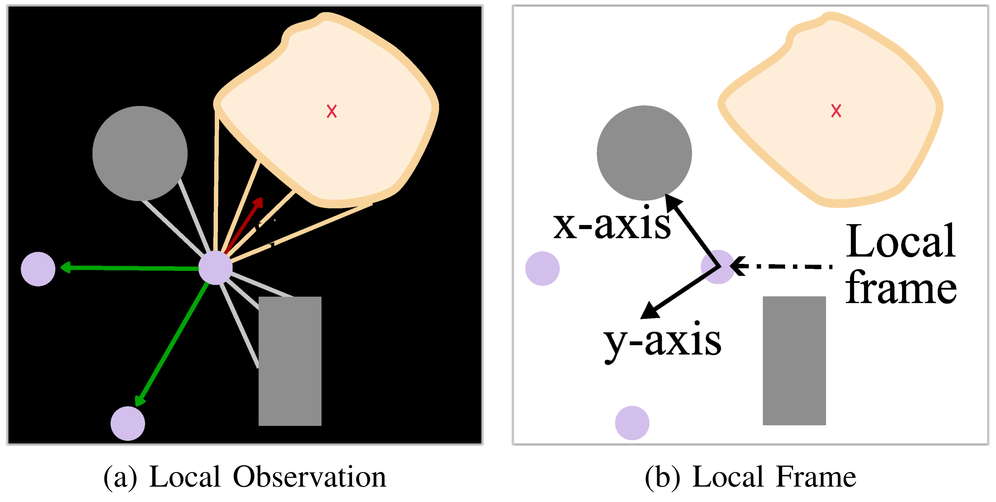
Original panel labels
III-B Problem Formulation
A partially observable Markov game defines joint transitions, individual rewards and local policy inputs. Each robot maximizes discounted reward under its stochastic policy. Equations 1–2 retain the full game specification and objective; the partial-observation formulation does not itself restrict communication range.
Equations 1–2
| (1) |
| (2) |
III-C Agents, Observations and Actions
Unicycle robots output linear and angular velocities. Their inputs include position, velocity, estimated current load, every other robot’s relative position and load, twelve obstacle/robot distance rays, twelve target-boundary rays and a team load-similarity score. Figure 3 expresses vectors in each robot’s local coordinate frame.
Obstacle sensing is range-limited, but teammate information covers all other robots and the score aggregates team loads. Decentralized action selection therefore does not mean communication-free or strictly local-neighbor sensing. The observation dimension changes with team size.
Equations 3–9
| (3) |
| (4) |
| (5) |
| (6) |
| (7) |
| (8) |
| (9) |
III-D Load Computation and Sharing
Only robot centers inside the polygon participate. The load model enforces total vertical force and zero moments about the object’s center of mass, solving the linear system by least squares or a pseudoinverse. It normalizes the resulting loads and pads outside robots with zeros. A scaled cosine similarity to uniform loads supplies the team score; α=2 and exponent β=10 emphasize near-uniform configurations.
This is an unconstrained static surrogate. Negative loads are possible and would require pulling the object downward; nonnegative contact forces, actuator limits and exact equilibrium feasibility are not enforced by the stated solve. The simplification in Equations 16–18 assumes unit-sum normalized loads and suppresses the preceding numerical stabilizers. The score is not a physical support certificate.
Equations 10–18
| (10) |
| (11) |
| (12) |
| (13) |
| (14) |
| (15) |
| (16) | ||||
| (17) | ||||
| (18) |
III-E Reward Design
Rewards combine footprint entry/progress, collision penalty, load similarity and a bonus when all robots are inside and the score exceeds a team-size threshold. The stated intention is to attract robots toward the object while encouraging balanced support.
A source sign discrepancy is retained: Equation 20 uses αₚ(dₚᵗ−dₚᵗ⁻¹) outside the footprint, with positive αₚ=0.1. For the nonnegative distance defined in the text, that term rewards moving farther away, contrary to the prose. The displayed formula alone does not establish what the implementation executes.
Equations 19–21
| (19) |
| (20) |
| (21) |
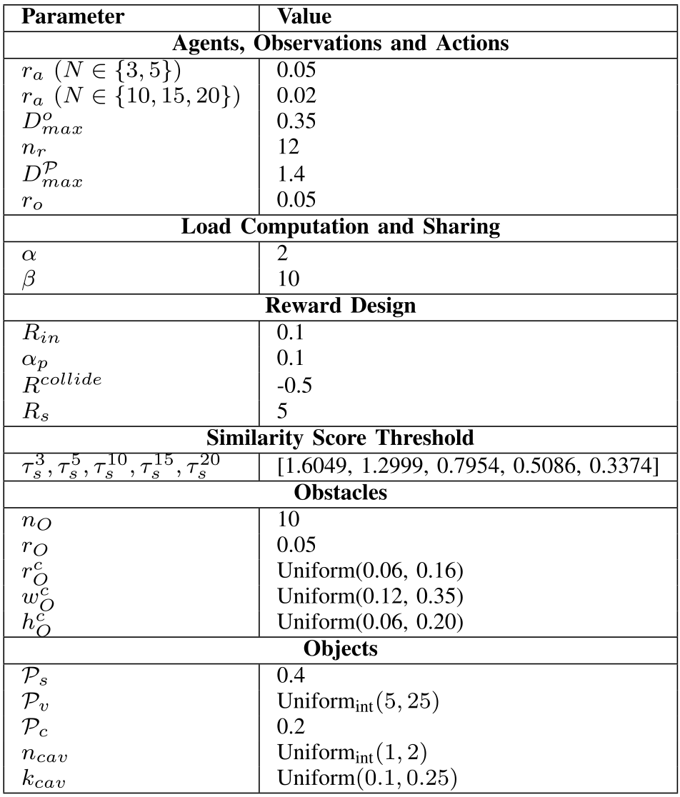
Original selectable table
| Parameter | Value |
|---|---|
| Agents, Observations and Actions | |
| 0.05 | |
| 0.02 | |
| 0.35 | |
| 12 | |
| 1.4 | |
| 0.05 | |
| Load Computation and Sharing | |
| 2 | |
| 10 | |
| Reward Design | |
| 0.1 | |
| 0.1 | |
| -0.5 | |
| 5 | |
| Similarity Score Threshold | |
| [1.6049, 1.2999, 0.7954, 0.5086, 0.3374] | |
| Obstacles | |
| 10 | |
| 0.05 | |
| Uniform(0.06, 0.16) | |
| Uniform(0.12, 0.35) | |
| Uniform(0.06, 0.20) | |
| Objects | |
| 0.4 | |
| 0.2 | |
Original selectable table
| Parameter | Search Space | Chosen Value |
|---|---|---|
| LogUniform() | ||
| Uniform() | ||
| LogUniform() | ||
| Uniform() | ||
| , | ), | |
III-F Similarity Score Threshold Choice
The paper derives a similarity threshold from a desired maximum normalized-load spread d=0.15. Its intermediate case assumes one high load and all remaining loads equally low. The original endpoint cases and derivation are preserved below.
That threshold is not equivalent to bounding the largest load difference. For five robots, the derivation uses squared norm 0.218 and threshold about 1.2999. Loads [0.29, 0.11, 0.20, 0.20, 0.20] sum to one and pass the score test, although their spread is 0.18. Conversely, [0.29, 0.29, 0.14, 0.14, 0.14] have allowed spread 0.15 but lower similarity and fail. Thus the reported score criterion must be distinguished from a proven 0.15 spread guarantee; these counterexamples concern the formula, not reconstructed experimental trajectories.
Equations 22–26
| (22) |
| (23) |
| (24) |
| (25) | |||
| (26) |
III-G Policy Optimization
MAPPO extends PPO with a centralized value function. Homogeneous robots share a three-layer ReLU actor producing a diagonal Gaussian action, squashed through tanh to respect velocity bounds. A two-layer critic receives concatenated team observations and predicts a value for each robot; generalized advantage estimates drive policy updates. Sharing actor parameters is within a fixed-size team, not demonstrated transfer of one policy across sizes.
IV EXPERIMENTAL SETUP
IV-A Environment
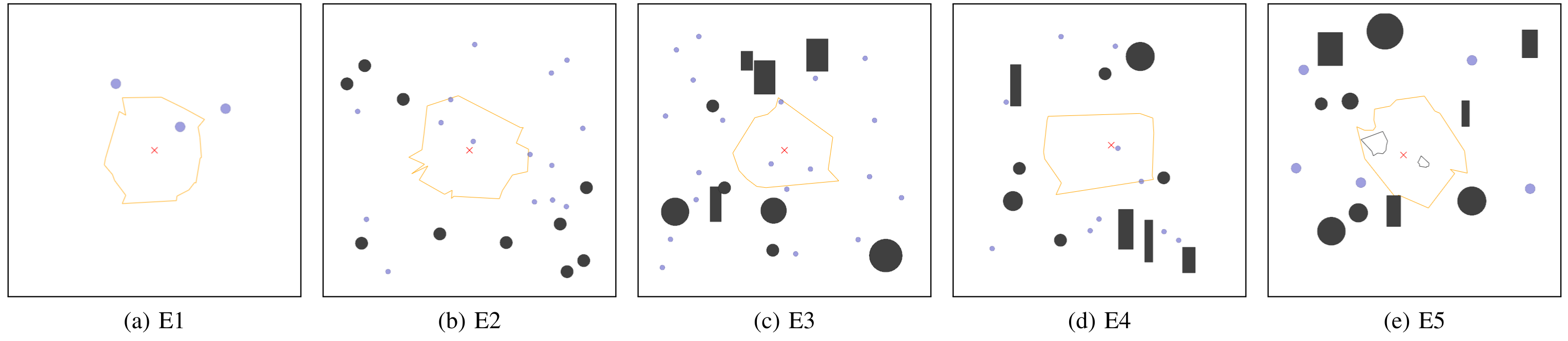
VMAS supplies the two-dimensional dynamics. E1 uses random star-shaped polygons without obstacles; E2 adds circles; E3 uses denser circular/rectangular clutter. E4 shifts the center of mass and E5 adds cavities. Random radial perturbations control polygon concavity; the center-of-mass shift models nonuniform weight without simulating a lifted three-dimensional load.
Table I retains all scene and reward parameters. Robot radius changes from 0.05 for three/five robots to 0.02 for larger teams, so scaling comparisons also change physical packing difficulty. These tests sample the same families used in training, rather than unrestricted arbitrary objects.
Equation 27
| (27) |
IV-B Hyperparameters
Separate policies are trained for 3, 5, 10, 15 and 20 robots. Training uses 150 parallel scenes, 125 updates and seed zero, with randomized clutter, shifted centers of mass and cavities appearing with probability 0.35. Two hundred steps per rollout gives 3.75 million environment steps; the larger teams use 300-step rollouts, so the same update count would imply 5.625 million steps rather than the stated common total.
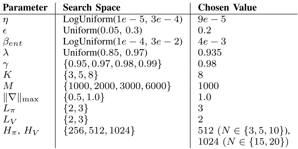
A Ray Tune search tests 64 configurations per team size for fifty iterations, selecting by mean episode reward. Adam jointly updates actor/critic with per-robot advantage normalization and gradient clipping. The chosen widths are 512 for smaller teams and 1,024 for fifteen/twenty robots. Table II preserves the full search spaces and selected settings; multi-seed robustness is not reported.
IV-C Post-Evaluation
Each team/environment combination is evaluated in 150 runs capped at 400 steps. Reported success uses the footprint/score threshold; mean execution steps measures time to the successful formation. The paper describes this as equivalent to maximum load spread below 0.15, but the preceding threshold derivation does not justify that equivalence. No transported distance or carried-object collision metric is measured.
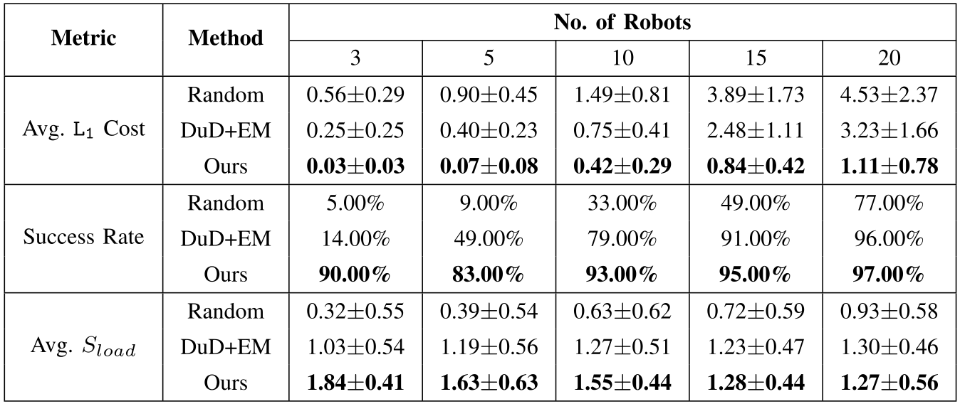
Baselines are random placements and DUD+EM: an attraction/repulsion field fills the shape, followed by centroid-based refinement. A separate comparison runs each method one hundred times on obstacle-free unions of two to five rectangles with shifted centers of mass. A mixed-integer linear program finds the closest equal-load, minimum-spacing formation using total Manhattan distance. This restricted benchmark measures formation correction cost, not a transport trajectory; objects are doubled in size for fifteen/twenty robots.
V RESULTS
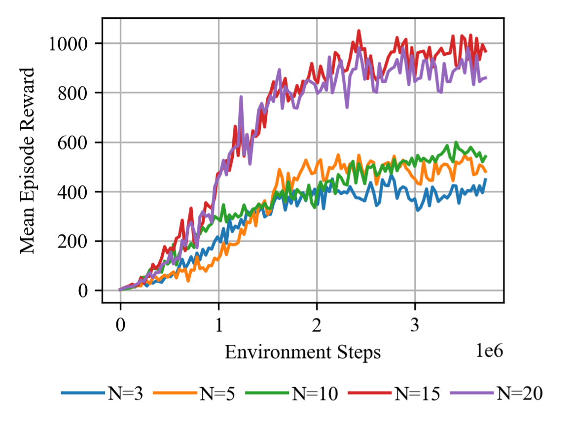
The learning curves and all tabulated outcomes below are retained as reported. Interpretation depends on the fixed-size policies, simulator load surrogate and score-based success rule.
V-A Policy Optimization
Returns improve for all five team sizes. Three robots have less geometric redundancy for balancing moments; larger teams can redistribute the estimated load more easily. Fifteen/twenty robots also train with longer episodes, accumulating more shaping and success reward, so their raw returns are not directly comparable with smaller teams. The curves provide one-seed training evidence rather than confidence intervals over independent training runs.
V-B Post-Evaluation
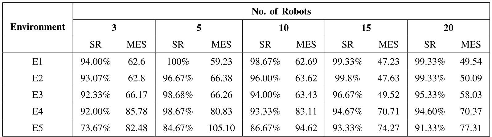
Table III reports 92–100% success over E1–E4. Cavities reduce E5 success to 73.67%, 84.67%, 86.67%, 93.33% and 91.33% for increasing team sizes. Corresponding mean formation steps are 82.48, 105.10, 94.62, 74.27 and 77.31. These are formation outcomes under the reported threshold, not successful physical transports.
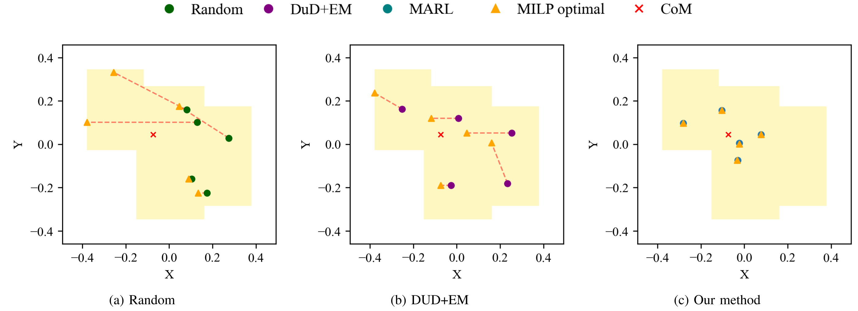
In the separate rectangle-union benchmark, learned formations have lower mean correction cost than both baselines for every size: 0.03/0.07/0.42/0.84/1.11 versus DUD+EM’s 0.25/0.40/0.75/2.48/3.23. Success is 90/83/93/95/97%, versus 14/49/79/91/96%. However, at twenty robots DUD+EM has slightly higher mean similarity, 1.30 versus 1.27; the proposed method does not lead every metric.
Figure 6 shows five robots, matching its caption despite the body’s “ten robots” wording. Several Table III percentages, including 99.8%, do not correspond to integer successes out of the stated 150 runs; the paper does not explain that aggregation. The figures and values remain unchanged. Lower correction costs support the sampled formations’ quality, without establishing an optimality guarantee for the policy.
Original selectable table
| Environment | No. of Robots | |||||||||
|---|---|---|---|---|---|---|---|---|---|---|
| 3 | 5 | 10 | 15 | 20 | ||||||
| SR | MES | SR | MES | SR | MES | SR | MES | SR | MES | |
| E1 | 94.00% | 62.6 | 100% | 59.23 | 98.67% | 62.69 | 99.33% | 47.23 | 99.33% | 49.54 |
| E2 | 93.07% | 62.8 | 96.67% | 66.38 | 96.00% | 63.62 | 99.8% | 47.63 | 99.33% | 50.09 |
| E3 | 92.33% | 66.17 | 98.68% | 66.26 | 94.00% | 63.43 | 96.67% | 49.52 | 95.33% | 58.03 |
| E4 | 92.00% | 85.78 | 98.67% | 80.83 | 93.33% | 83.11 | 94.67% | 70.71 | 94.60% | 70.37 |
| E5 | 73.67% | 82.48 | 84.67% | 105.10 | 86.67% | 94.62 | 93.33% | 74.27 | 91.33% | 77.31 |
Original selectable table
| Metric | Method | No. of Robots | ||||
|---|---|---|---|---|---|---|
| 3 | 5 | 10 | 15 | 20 | ||
| Avg. Cost | Random | 0.560.29 | 0.900.45 | 1.490.81 | 3.891.73 | 4.532.37 |
| DuD+EM | 0.250.25 | 0.400.23 | 0.750.41 | 2.481.11 | 3.231.66 | |
| Ours | 0.030.03 | 0.070.08 | 0.420.29 | 0.840.42 | 1.110.78 | |
| Success Rate | Random | 5.00% | 9.00% | 33.00% | 49.00% | 77.00% |
| DuD+EM | 14.00% | 49.00% | 79.00% | 91.00% | 96.00% | |
| Ours | 90.00% | 83.00% | 93.00% | 95.00% | 97.00% | |
| Avg. | Random | 0.320.55 | 0.390.54 | 0.630.62 | 0.720.59 | 0.930.58 |
| DuD+EM | 1.030.54 | 1.190.56 | 1.270.51 | 1.230.47 | 1.300.46 | |
| Ours | 1.840.41 | 1.630.63 | 1.550.44 | 1.280.44 | 1.270.56 | |
VI CONCLUSION
Adding load-aware reward improves simulated support placement beyond geometric shape filling. The evidence is limited to two-dimensional formation, estimated unconstrained loads, one training seed and separately trained team sizes. Collision penalties and favorable success rates do not certify safe support or navigation.
The authors identify full transport after lifting, onboard geometry/mass estimation and graph-based policies for larger teams as future work. Those additions would be needed to test the method’s assumptions on physical robots and more scalable communication structures.
ACKNOWLEDGEMENTS
The authors acknowledge support from the German research ministry through Robotics Institute Germany and computing resources from NHR@FAU under BayernKI.