Overview
MosaicIMU combines carrier-conditioned inertial velocity learning with a filter that maintains past poses. The complete derivation, training splits, carrier-level results, adaptation ablations, and hardware specifications are retained below. Project code.
At a glance
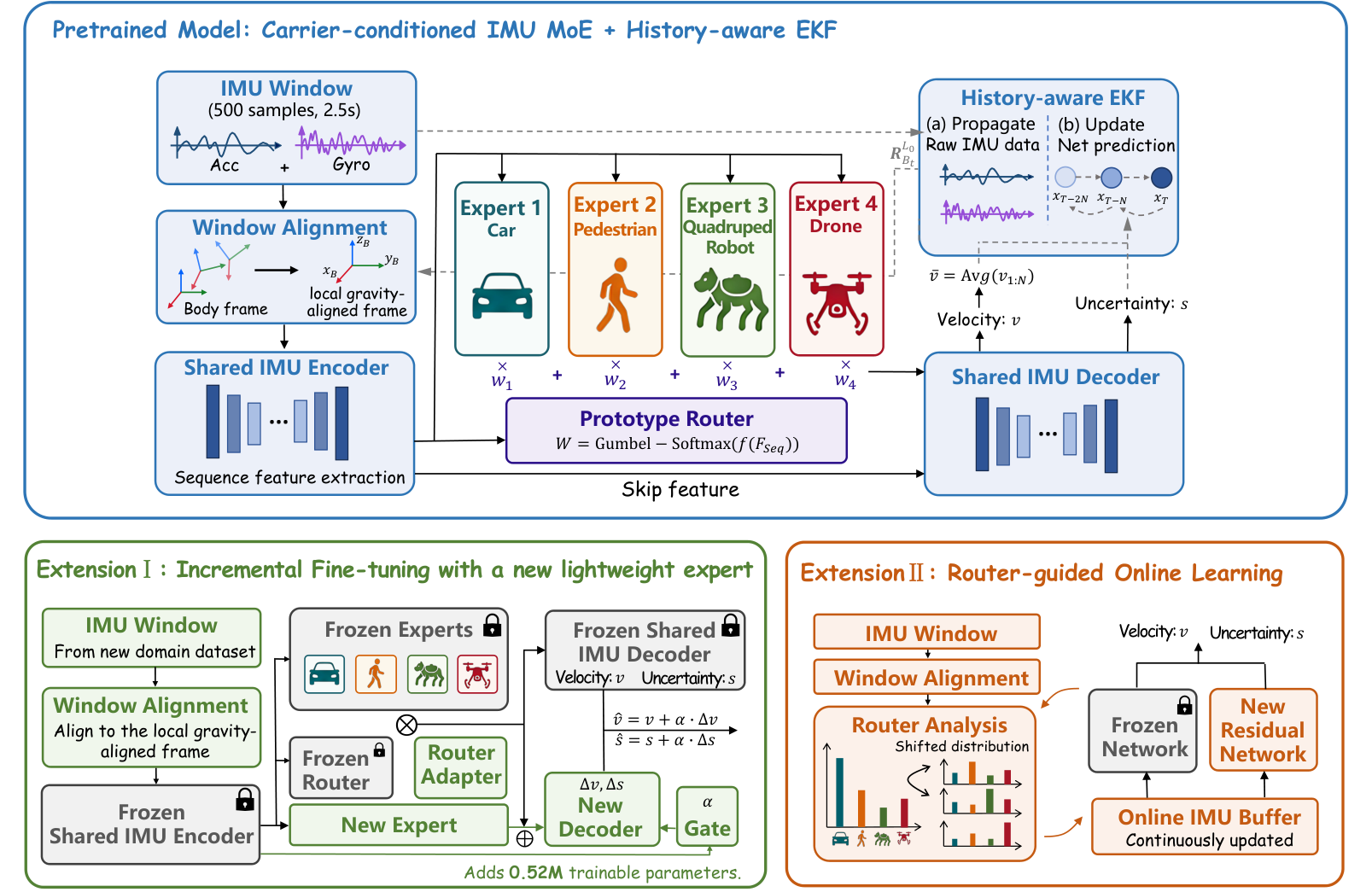
A shared encoder and four carrier experts predict local velocity and uncertainty from inertial windows. A prototype router mixes their features before decoding, and an error-state filter turns the predictions into trajectory constraints. Across held-out vehicle, quadruped, pedestrian, and drone sequences, average position error falls from the strongest baseline’s 6.95 m to 4.15 m and ten-second relative error from 1.98 m to 1.31 m. Frozen-base residual adaptation helps a new mounting/domain. These are four-carrier results, with external reference supervision required for the demonstrated online adaptation.
1 Introduction
Motion priors can reduce inertial integration drift, but priors learned for one carrier may fail on another. MosaicIMU shares and composes carrier-specific features rather than selecting a fixed output head. Its contributions combine representation, probabilistic filtering, a small adaptation branch, and router-based online sample selection. The experiments support improved average performance on the tested domains; they do not establish arbitrary unseen-carrier or hardware generalization.
2 Related Work
The method brings together learned inertial motion priors, multi-carrier pretraining, and state estimation that treats neural outputs as relative constraints.
Learning-based inertial odometry.
Classical integration accumulates bias, noise, and gravity-compensation errors. Learned displacement or velocity from short windows can constrain that drift. Recurrent, convolutional, attention-based, and equivariant designs improve particular regimes, but most prior models specialize in a carrier or motion distribution.
Carrier-specific and multi-carrier inertial learning.
Pedestrian gait, vehicle kinematics, leg contact, and aerial dynamics provide different useful priors. TartanIMU shares pretraining across carriers while retaining separate output heads. MosaicIMU instead mixes expert features for each input before a shared decoder, allowing complementary experts to contribute.
Estimator-compatible learning-based inertial constraints.
TLIO combines learned displacement and uncertainty with inertial filtering; related methods integrate neural constraints into visual-inertial or factor-graph estimators. MosaicIMU predicts dense velocities in a window-fixed gravity-aligned frame and averages them into a relative constraint between historical poses.
3 Method
The pretrained model provides four-carrier velocity priors and a history-aware filter. Offline adaptation freezes the base and trains a router correction plus a gated residual branch. Online adaptation trains those same small components from a selected buffer as new supervised windows arrive.
3.1 Carrier-Conditioned Mixture-of-Experts Network
The network first aligns each window to a stable local frame, then combines carrier-conditioned features and jointly predicts velocity and diagonal uncertainty. Carrier priors regularize routing without making the output strictly one-hot.
Local gravity-aligned IMU representation.
Each 2.5-second window uses a gravity-aligned frame whose yaw is anchored to the body heading at the window start. Acceleration, angular velocity, and velocity targets are expressed consistently in that frame. This removes dependence on an arbitrary global yaw reference, but still requires sufficiently reliable attitude propagation; it is not attitude-free inertial estimation.
Equation 1
| (1) |
Carrier-conditioned feature fusion.
The shared encoder produces temporal features and two skip features. A router compares its embedding with four learned prototypes using scaled cosine similarity, then applies Gumbel-Softmax. Weighted expert features pass through a shared decoder to dense velocity and variance sequences. The four prototypes correspond to vehicles, pedestrians, quadrupeds, and drones; mixing occurs before the output, not by selecting separate final heads.
Equations 2–4
| (2) |
| (3) |
| (4) |
Training objective.
Training adds heteroscedastic Gaussian negative log-likelihood, an unweighted squared velocity error, prototype-separation regularization, and a carrier-prior divergence. The diagonal variance controls uncertainty weighting; the direct velocity term maintains explicit regression supervision. Absolute pairwise prototype cosine similarity discourages collapse, while the prior term encourages carrier semantics without eliminating soft composition.
Equations 5–8
| (5) |
| (6) |
| (7) |
| (8) |
3.2 Segment-Level Velocity Constraints for History-Aware EKF
The filter propagates orientation, velocity, position, and two sensor biases from raw IMU data while storing bounded historical pose clones. A full prediction window contributes one mean local-velocity observation between its endpoint clones. The prediction is compared with endpoint displacement divided by elapsed time in the same yaw-anchored frame. Approximate observation covariance sums frame variances with squared averaging weights, neglecting temporal cross-correlation. This is a relative trajectory constraint, not an absolute heading measurement.
Equations 9–10
| (9) |
| (10) |
3.3 Incremental Fine-tuning with a New Lightweight Expert
Adaptation freezes the pretrained encoder, experts, router, and decoder. A small adapter adds corrections to router logits, and a new expert/decoder predicts residual velocity and variance. A sigmoid gate scales the residual; softplus keeps the variance increment nonnegative. The base objective is reused without prototype orthogonality. Preserving base weights limits direct forgetting, while changed routing and residual outputs can still affect source-domain predictions.
Equations 11–14
| (11) |
| (12) |
| (13) |
| (14) |
3.4 Router-Guided Online Adaptation
For a known expected carrier, mismatch is one minus that carrier’s calibrated routing weight. The highest-scoring windows fill a small training subset for updating the adapter and residual branch. This score is a routing-based selection heuristic, not a demonstrated calibrated uncertainty estimate. In the vehicle experiment, external reference velocities supervise the selected windows.
Equations 15–16
| (15) |
| (16) |
4 Experimental Results
Evaluation covers four-carrier held-out trajectories, supervised adaptation to an excluded head-mounted dataset, and one campus-vehicle online adaptation setting. Position, ten-second relative displacement, and vertical errors measure different aspects of drift. All original numerical tables and trajectory panels remain available.
4.1 Generalization of the Pretrained MosaicIMU
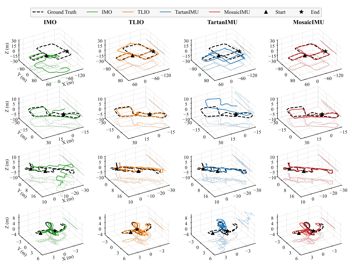
IMO and TLIO are each trained separately for every carrier, while TartanIMU and MosaicIMU share multi-carrier training data. Table 1 gives average ATE/RTE of 4.15/1.31 m for MosaicIMU versus TLIO’s 6.95/1.98 m and TartanIMU’s 11.94/3.10 m. The headline 40%/34% reductions use TLIO’s averages. MosaicIMU has better average error, but quadruped ATE is 2.01 m versus TLIO’s 1.74 m.
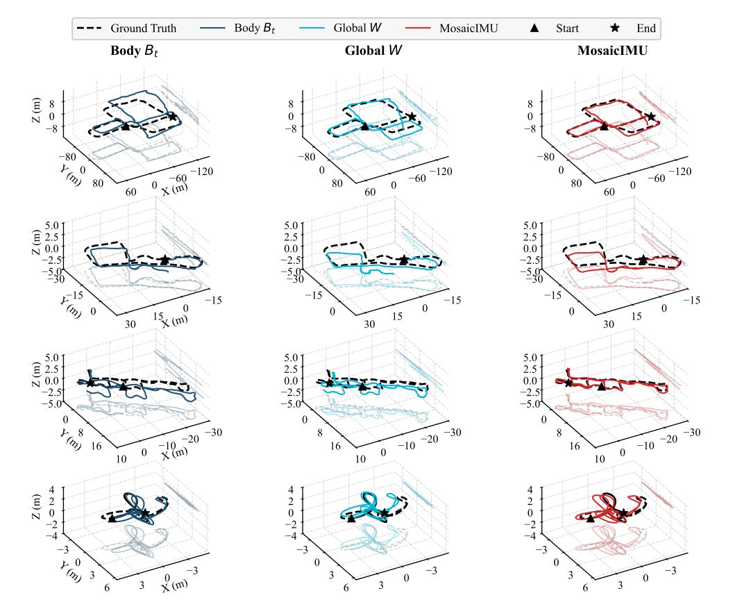
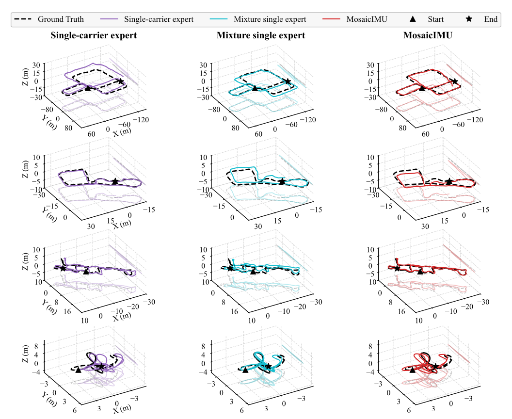
Prediction-frame ablations average 8.00 m ATE in the body frame, 10.40 m globally, and 4.15 m locally gravity-aligned. Independent single-carrier experts and a single mixed expert average 5.47 m and 5.53 m. These results favor the complete design in this benchmark; comparisons with TartanIMU also change the filtering interface, so they do not isolate routing alone.
| Carrier | IMO | TLIO | TartanIMU | MosaicIMU | ||||
|---|---|---|---|---|---|---|---|---|
| ATE | RTE-10s | ATE | RTE-10s | ATE | RTE-10s | ATE | RTE-10s | |
| Vehicle | 156.02 | 13.11 | 20.87 | 3.68 | 25.44 | 2.77 | 10.56 49% | 2.17 22% |
| Quadruped | 3.49 | 1.22 | 1.74 | 0.79 | 3.44 | 1.17 | 2.01 16% | 0.63 20% |
| Pedestrian | 11.91 | 6.21 | 3.83 | 1.95 | 10.12 | 2.39 | 2.85 26% | 1.28 34% |
| Drone | 1.29 | 1.17 | 1.37 | 1.48 | 8.74 | 6.08 | 1.17 9% | 1.14 3% |
| Average | 43.18 | 5.43 | 6.95 | 1.98 | 11.94 | 3.10 | 4.15 40% | 1.31 34% |
4.2 Incremental Fine-tuning with a New Lightweight Expert on Unseen Domains
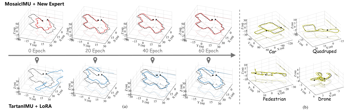
The head-mounted TLIO dataset is excluded from pretraining. Updating 0.52 million MosaicIMU parameters lowers ATE from 9.85 m to 2.60 m at twenty epochs and 1.49 m at sixty. TartanIMU with 0.74 million LoRA parameters starts at 54.27 m and reaches 5.97 m. The lower starting error and different adaptation designs both influence this comparison. Source-domain trajectory plots suggest retention after adaptation, without a quantitative forgetting guarantee across all domains.
4.3 Router-Guided Online Adaptation
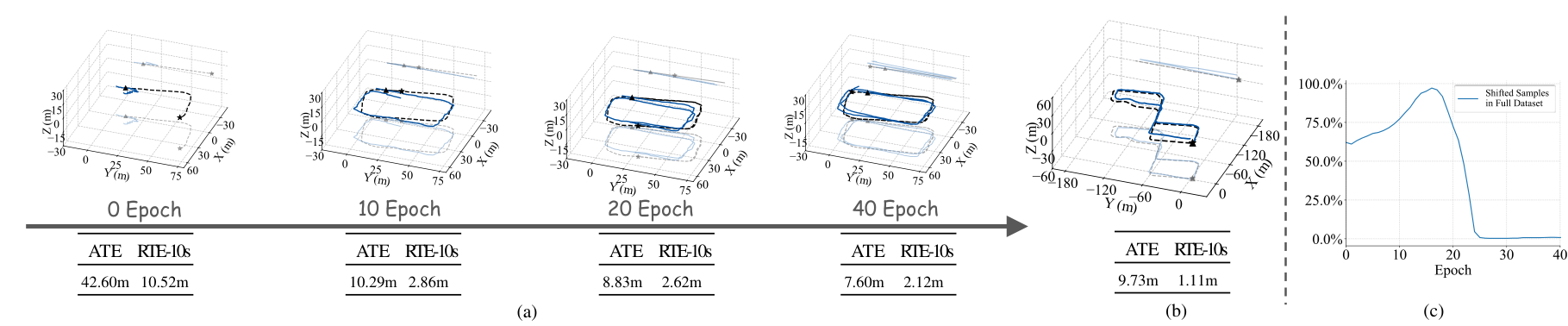
The campus vehicle uses DLIO LiDAR-inertial velocity supervision during online learning, and reference filter updates during warm-up. Once adapted, inference and filter constraints use IMU data alone. Reported epoch scores replay the collected trajectory with each checkpoint against DLIO’s trajectory, rather than measuring continuously changing closed-loop estimation against independent ground truth.
ATE decreases from 42.60 m to 10.29 m at ten epochs and 7.60 m at forty; ten-second relative error falls from 10.52 m to 2.12 m. A separate same-domain sequence gives 9.73/1.11 m. The proportion of buffered samples with vehicle weight below 0.8 falls to zero around epoch twenty-five, but top-ranked selection and replay continue; this does not mean all online learning stops then.
5 Limitations
Training covers only four carrier categories at limited scale. New hardware, mounting, or an entirely unseen carrier can shift the distribution, and broad zero-shot transfer has not been systematically tested. Severe bias changes or poor attitude propagation can destabilize the filter. Online adaptation currently requires reference supervision early on; self-supervised adaptation and stronger uncertainty estimation remain future work.
6 Conclusion
Composing carrier features and using local, historical velocity constraints improves the tested average trajectory errors. Small residual adaptation transfers to a new head-mounted dataset and a supervised campus-vehicle domain. The evidence supports this pretraining-plus-adaptation pipeline within the reported settings, while broader carrier, sensor, and long-deployment robustness remains open.
Acknowledgments
The authors acknowledge support from the State Key Laboratory of Autonomous Intelligent Unmanned Systems, the Tsinghua–Toyota Joint Research Fund, and the National Natural Science Foundation of China.
Appendix
The appendices specify training, the complete filter formulation, dataset splitting, baseline interfaces, all metrics and ablations, and online hardware and replay details.
Appendix A Method
Implementation details connect the learning objective to a bounded-history error-state estimator. All numbered equations and the yaw-invariance identity are retained.
A.1 Details of Training
Training uses one RTX 4090, 200 Hz resampling, 500-frame windows with 250-frame stride, and six inertial channels. The base trains for one hundred epochs with batch size 128, Adam, weight decay 10⁻⁴, and a cosine learning-rate schedule from 10⁻³ to 10⁻⁵. Inputs and velocity labels share the local gravity-aligned frame.
A.2 Details of History-Aware EKF
The estimator follows stochastic cloning and multi-state constraint filtering. Its distinguishing interface aggregates dense learned local velocities into a segment observation between cloned poses. The following derivation retains state conventions, propagation, clone covariance, measurement Jacobians, correction, and removal of old states.
State and perturbation convention.
The current state has orientation, velocity, position, gyroscope bias, and accelerometer bias. Each stored clone adds orientation and position. Rotations use a left-multiplicative error and positions an additive one, giving a covariance dimension of fifteen plus six times the clone count. Those conventions determine the signs and blocks in the retained Jacobians.
Equations 17–21
| (17) |
| (18) |
| (19) |
| (20) |
| (21) |
IMU propagation.
Bias-corrected angular velocity propagates rotation; rotated acceleration and gravity propagate velocity and position. Nominal biases stay fixed during each step while covariance models bias random walks. The transition and noise Jacobians preserve coupling between attitude, acceleration, velocity, position, and biases, rather than treating neural velocity as an independent position integrator.
Equations 22–27
| (22) |
| (23) | ||||
| (24) |
| (25) | ||||||
| (26) |

Pose cloning.
A pose is cloned every fixed number of IMU samples. Once a full window and enough clones exist, the newest clone pairs with the window’s starting clone for one update. Clone augmentation selects attitude and position rows from the propagation transition and inherits cross-covariances. The oldest clone is removed after correction, bounding memory while retaining the correlations needed by the next segment.
Equations 28–31



| (31) |
Filter-aware aggregation of dense neural velocities.
The prediction length equals the number of clone intervals times their sampling stride, so neural averaging and pose displacement span the same interval. Uniform weights give one mean velocity per complete window. Both sides use the starting clone’s yaw anchor. The variance formula explicitly neglects cross-covariance between framewise errors; dense overlapping predictions should not be interpreted as independently measured physical velocities.
Equations 32–36
| (32) |

| (34) |
| (35) |
| (36) |
Velocity-consistency measurement model.
The filter’s expected observation is endpoint position difference divided by elapsed time, rotated into the window’s local frame. The residual compares this state-dependent segment velocity with the neural average. It therefore constrains the maintained trajectory through historical states, rather than simply integrating the network output.
Equations 37–39
| (37) |
| (38) |
| (39) |
Yaw consistency.
Applying the same arbitrary global yaw rotation to both endpoint positions and the local-frame anchor leaves the predicted observation unchanged. This invariance holds when the neural observation uses the same anchor. It avoids injecting an explicit absolute-heading observation, without removing the need to estimate gravity alignment and relative attitude.
Equation
Measurement Jacobian.
Only the initial clone’s yaw-dependent orientation block and the two endpoint position blocks enter the direct measurement Jacobian. The derivation maps left attitude perturbations through a yaw-extraction Jacobian and retains all signs, frame rotations, and time scaling. Other direct blocks are zero, but covariance cross-terms allow the update to influence other states.
Equations 40–46
| (40) |
| (41) |
| (42) |
| (43) |
| (44) |
| (45) |
| (46) |
Kalman update and marginalization.
Innovation covariance and Kalman gain produce corrections for clones and the current inertial state, including biases. The stated covariance update is followed by explicit symmetrization. Deleting the oldest clone’s entries and matching covariance rows/columns maintains bounded size. Intermediate states still receive corrections through their cross-correlations with the measured endpoints.
Equations 47–51
| (47) |
| (48) |
| (49) | ||||||
| (50) |
| (51) |
Discussion.
Dense supervision lets the network learn fine temporal motion cues, while segment averaging provides a less frame-noise-sensitive filter interface. The estimator combines learned motion priors with inertial propagation. Its practical robustness still depends on the learned uncertainty approximation, stable attitude estimation, and the motion distributions represented in training.
Appendix B Experimental Results
The experimental appendix supplies source datasets, disjoint split rules, baseline implementation differences, metric definitions, carrier-level ablations, and the supervised online adaptation procedure.
B.1 Multi-Carrier IMU Training Datasets
Eight datasets cover vehicles, quadrupeds, pedestrians, and drones, with carrier reweighting to approximately equal training contributions. Complete trajectories are split 9:1 before windowing. Held-out trajectories do not enter training, validation, tuning, or normalization. Within each training trajectory, the first 5% and last 15% form validation segments and the middle 80% trains the model.
Window extraction follows segmentation; boundary-crossing windows and a one-window margin are removed to avoid shared raw samples. Resampling and window sizes match Appendix A. Gaussian measurement noise and joint yaw rotation of IMU windows and velocity targets augment noise and heading without altering gravity direction.
| Carrier | Dataset | Duration | Environment |
|---|---|---|---|
| Vehicle | i2Nav-Robot [28] | 4h | Indoors, Outdoors |
| SubT-MRS [30] | 3h | In/Outdoors, Underground | |
| Quadruped | CEAR [34] | 4h | Indoors, Outdoors |
| Cerberus [29] | 2h | Underground | |
| Pedestrian | IDOL [27] | 5.4h | Indoors |
| RNIN-VIO [8] | 5h | Indoors, Outdoors | |
| Drone | BlackBird [2] | 1h | Indoors |
| MILUV [26] | 3.6h | Indoors |
B.2 Details of Compared Baselines
IMO and TLIO each use four separately trained carrier models; TartanIMU and MosaicIMU use the same multi-carrier datasets. All evaluate identical held-out sequences. IMO’s original drone formulation takes collective thrust and gyroscope signals; the paper describes training carrier-specific versions without fully detailing the non-drone thrust-input adaptation.
TLIO predicts displacement and uncertainty for an error-state filter. TartanIMU predicts body-frame velocity and uses a standard velocity-observation filter here, whereas MosaicIMU uses the proposed historical relative constraint. The comparison therefore includes representation and estimator changes as well as expert architecture.
Excluded methods.
AI-IMU is excluded because its vehicle-oriented kinematic assumptions do not apply uniformly across carriers. RoNIN is excluded for dependence on approximate external attitude priors. This defines a selected baseline set; MosaicIMU also requires adequate attitude propagation, so the exclusions do not establish universal superiority over all inertial-odometry approaches.
B.3 Evaluation Metrics
All reported errors use estimated and reference world-frame positions and are expressed in metres. The following definitions distinguish whole-trajectory position error, ten-second displacement error, and vertical position error.
Absolute Trajectory Error (ATE).
Absolute trajectory error is the root mean squared three-dimensional position discrepancy across evaluated timestamps. It measures accumulated position error rather than a drift rate per unit distance.
Equation 52
| (52) |
Relative Trajectory Error over 10 seconds (RTE-10s).
Ten-second relative trajectory error compares estimated and reference displacements over windows separated by ten seconds, then takes the root mean squared difference. It measures local displacement drift rather than absolute final position.
Equation 53
| (53) |
Vertical trajectory error ( z -Drift).
The reported z-Drift is root mean squared vertical position error over the trajectory, equivalent to restricting ATE to the world z coordinate. Despite its name, it is not a vertical bias-growth rate.
Equation 54
| (54) |
B.4 Ablation Studies of Pretrained MosaicIMU
Three ablation groups vary the velocity coordinate frame, the expert architecture, and soft versus carrier-only routing. Complete per-carrier tables accompany the average results, revealing exceptions hidden by aggregates.
Ablation on prediction in different frames.
The local gravity-aligned representation improves all tabulated carrier/frame comparisons: average ATE is 4.15 m versus 8.00 m for body-frame and 10.40 m for global-frame prediction. Relative error is 1.31 versus 1.93/2.74 m, and vertical error is 0.73 versus 1.98/1.09 m. The source prose accidentally assigns 8.00 m to both alternatives; the unchanged table distinguishes them. A fixed window anchor stabilizes targets while preserving yaw consistency.
| Carrier | Body | Global | MosaicIMU | ||||||
|---|---|---|---|---|---|---|---|---|---|
| ATE | RTE-10s | -Drift | ATE | RTE-10s | -Drift | ATE | RTE-10s | -Drift | |
| Vehicle | 14.64 | 3.26 | 3.68 | 26.76 | 3.95 | 1.91 | 10.56 28% | 2.17 33% | 1.50 21% |
| Quadruped | 2.44 | 0.69 | 1.38 | 2.55 | 0.93 | 1.56 | 2.01 18% | 0.63 9% | 0.86 38% |
| Pedestrian | 13.47 | 2.16 | 1.92 | 9.12 | 3.89 | 0.65 | 2.85 69% | 1.28 41% | 0.35 46% |
| Drone | 1.44 | 1.62 | 0.92 | 3.17 | 2.18 | 0.25 | 1.17 19% | 1.14 30% | 0.22 12% |
| Average | 8.00 | 1.93 | 1.98 | 10.40 | 2.74 | 1.09 | 4.15 48% | 1.31 32% | 0.73 33% |
Ablation on expert design.
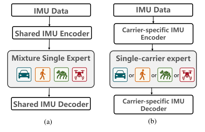
Independent carrier experts average 5.47 m ATE and 2.09 m relative error; one expert trained on all carriers averages 5.53/1.74 m. The routed mixture achieves 4.15/1.31 m and improves each carrier’s ATE and relative error in this ablation. The structural figure clarifies that both baselines use only one expert per prediction and no router.
| Carrier | Single-carrier expert | Mixture single expert | MosaicIMU | |||
|---|---|---|---|---|---|---|
| ATE | RTE-10s | ATE | RTE-10s | ATE | RTE-10s | |
| Vehicle | 14.12 | 3.09 | 14.14 | 3.21 | 10.56 25% | 2.17 30% |
| Quadruped | 2.14 | 1.37 | 2.42 | 0.69 | 2.01 6% | 0.63 9% |
| Pedestrian | 3.99 | 2.45 | 4.25 | 1.82 | 2.85 29% | 1.28 30% |
| Drone | 1.61 | 1.45 | 1.31 | 1.22 | 1.17 11% | 1.14 7% |
| Average | 5.47 | 2.09 | 5.53 | 1.74 | 4.15 24% | 1.31 25% |
Ablation on soft routing weights.
Hard one-hot routing selects the known carrier’s expert; soft routing allows other experts to contribute. Average ATE improves from 4.71 to 4.15 m and relative error from 1.34 to 1.31 m. All carriers improve in ATE, but pedestrian relative error worsens from 1.20 to 1.28 m. Thus the benefit is average and metric-dependent rather than uniform across every result.
B.5 Router Feature and Expert-Composition Analysis
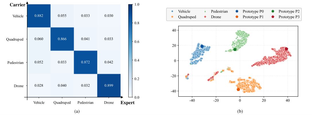
The average routing matrix is diagonal-dominant with nonzero off-diagonal weights, and the projected embeddings cluster near their carrier prototypes. These plots are consistent with carrier specialization plus shared features. They do not by themselves prove which borrowed features cause the error gains, or calibrate routing mismatch as uncertainty on an unseen domain.
B.6 Ablation Studies of the Lightweight Offline Fine-tuning
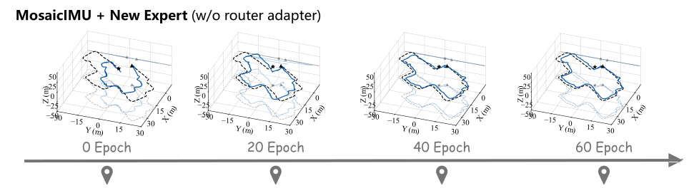
The ablation removes both the router adapter and the carrier-prior loss. With both components, twenty-epoch ATE is 2.60 m; without them it is 8.88 m, reaching 2.64 m only at sixty epochs. The full method reaches 1.49 m by sixty epochs. This supports the combined routing-calibration design, but cannot isolate the adapter’s effect from the simultaneously removed supervision term.
B.7 Details of Online Adaptation
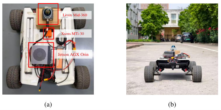
A vehicle with Xsens MTi-30 IMU, Livox Mid-360 LiDAR, and Jetson AGX Orin supplies the online experiment. DLIO generates supervision; the known carrier label supplies a vehicle prior. Every update recomputes mismatch scores and trains on the top sixty-four buffered windows while retaining prior observations for replay. Only the lightweight branch changes.
Each epoch takes under ten seconds on this platform. The vehicle completes the adaptation trajectory after roughly thirty epochs, followed by ten additional replay epochs. A separate same-domain trajectory is reserved for evaluation. The hardware table is retained in full; throughput here describes adaptation epochs, not a measured end-to-end inference latency guarantee.