Overview
This edition covers the complete twenty-three-page arXiv v2 dated 12 October 2026. It retains all ten numbered figures, thirteen numbered tables and the complete kinematic, data-generation and optimization appendix. Eight result tables whose HTML formatting failed are restored from the PDF.
At a glance
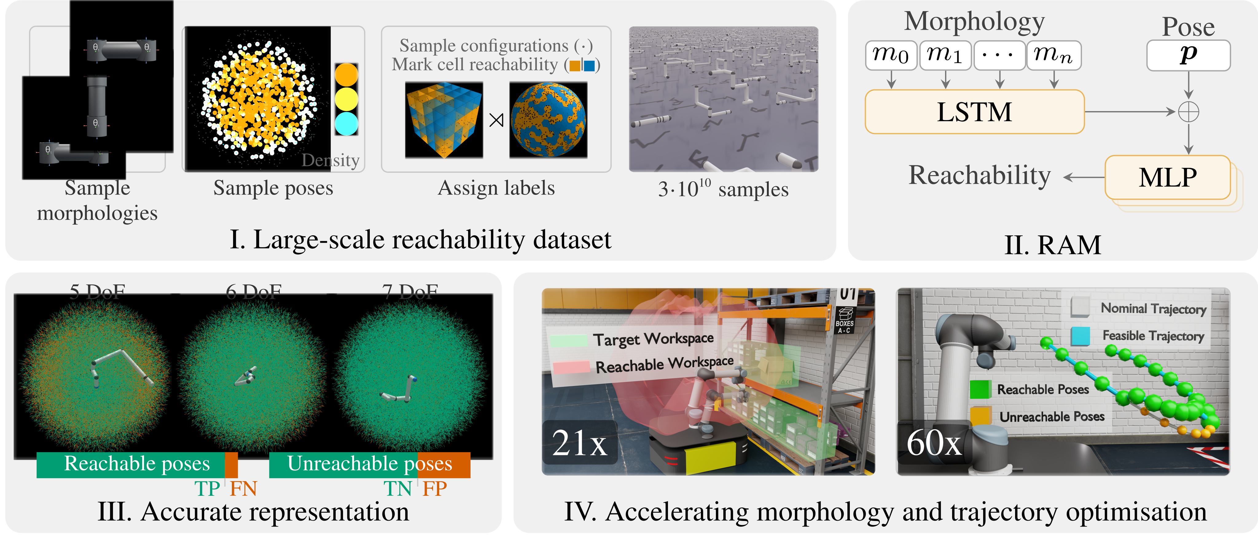
RAM predicts whether a robot morphology can reach an end-effector pose without self-collision. An LSTM encodes the kinematic chain and an occupancy network classifies the pose, avoiding an inverse-kinematics solve at each query.
Training uses thirty billion synthetic examples across thirty thousand morphologies. Reported balanced accuracy is 84%, versus 69% for a generative inverse-kinematics baseline; downstream optimization becomes faster but sacrifices reached-pose rate. The output is an approximate existence score, not a joint configuration or collision-free motion certificate.
1 Introduction
Repeated inverse-kinematics and self-collision queries make robot design and motion optimization expensive. Often an optimization step needs only to know whether some configuration exists; the actual joint solution is required later.
RAM learns a continuous morphology-conditioned workspace representation, building on occupancy networks and implicit neural representations. Large-scale forward-kinematics sampling supplies labels without an inverse solve for every training pose. The intended gain is fast, differentiable reachability queries across unseen designs.
2 Problem Statement
A pose is reachable if at least one inverse-kinematic solution is free of self-collision. The definition quantifies over the entire configuration set; it does not require all solutions to be safe.
The learned classifier approximates this existential predicate for a restricted morphology family. Later evaluations use a pose tolerance and finite solver-returned solutions, so their negative labels can miss valid solutions. Environmental obstacles are outside the definition used here.
Equations 1
| (1) |
3 Related Work
Analytical IKfast and EAIK exploit particular kinematic structures; numerical solvers handle broader chains but require iterative search. Learned GGIK predicts configurations through link positions, a richer problem than binary reachability.
Voxel reachability maps trade expensive precomputation and memory for fast lookup, but are tied to one morphology. Prior neural surrogates often cover one design or position-only reachability. RAM targets full position-and-orientation reachability across a restricted serial-chain family, including its capsule-based self-collisions.
4 Reachability Across Morphologies (RAM)
Synthesize a morphology, sample geometrically plausible poses and label them with a densely sampled workspace map. Train a binary classifier whose .5 level set approximates the boundary. This shifts computation to data generation and training; it does not eliminate workspace approximation error.
4.1 Morphology Sampling
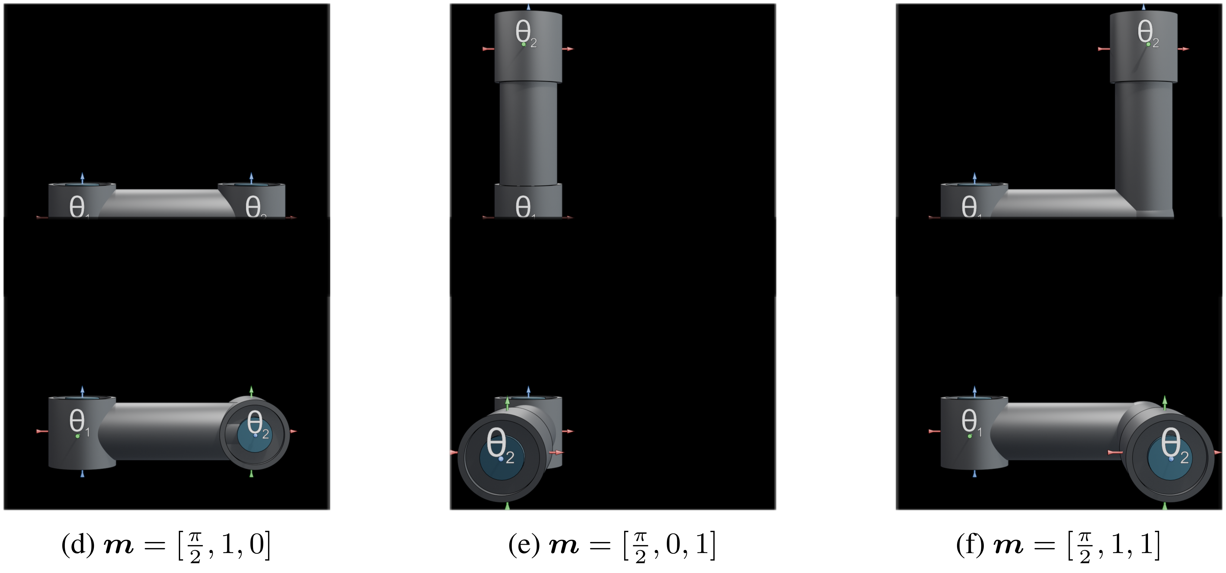
Training chains have five, six or seven revolute joints. Reject inoperable or functionally degenerate chains; successive axes must be parallel or orthogonal, with at most two co-located joints. Modified Denavit–Hartenberg triples encode twist, length and offset.
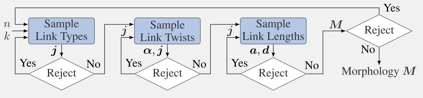
Normalize the sum of link-vector lengths to one and represent each link-joint pair by two fixed-radius capsules. Hierarchical rejection first checks topology, then twists and dimensions, avoiding expensive tests on already invalid candidates. Claimed uniform coverage is within this constructed, rejection-conditioned design space, not arbitrary robot geometries.
Equation
Selectable original panel labels
(a)
(b)
(c)
(d)
(e)
(f)
Equations
4.2 Pose Sampling
Sample positions in a reduced ball centered at the first joint, subtracting fixed base/end-effector lengths from movable reach, and sample orientation independently. Compose with the end-effector transform so obviously impossible far-away targets are excluded.
Five-degree-of-freedom workspaces have measure zero in six-dimensional pose space. Supplement their pose samples with forward-kinematic configurations to obtain positives. Consequently the evaluation distribution is deliberately constructed and its class balance is not a generic deployment prior.
Equations
4.3 Label Assignment
Discretize translation into cubes and orientation with iterative 600-cell tessellation plus a constant-time lookup. Sample joint configurations, compute forward kinematics, discard self-collisions, and mark a cell reachable if any surviving pose occupies it.
Unseen cells are negative under the closed-world assumption. Finite sampling can miss thin regions, while assigning an occupied cell’s label to every enclosed pose dilates the workspace. A colliding configuration never proves a pose unreachable because another configuration may be safe.
4.4 Training & Architecture
Represent a pose with three translations and six continuous rotation coordinates. A variable-length chain passes through an LSTM; concatenate its final embedding with the pose and use a ReLU MLP with sigmoid output. Train with binary cross-entropy.
Smooth dependence on continuous dimensions supports optimization, but the learned probability is not reported as calibrated. Discrete topology and link-twist choices are not differentiable design variables in the demonstrated optimizer.
Equations 2
| (2) |
5 Experiments
Evaluate label fidelity, unseen-morphology prediction and downstream optimization on an H100. Morphologies are balanced across joint counts and poses across morphologies; reported stochastic metrics use bootstrap 95% intervals, with seed averaging when multiple runs exist.
Validation/test labels use analytical solutions where available, otherwise collision-aware Levenberg–Marquardt with random restarts. A positive label has a feasible witness within tolerance; finite numerical search cannot certify every negative.
Equation 3
| (3) |
5.1 Label Fidelity (RQ1)
On ninety morphologies and nine million poses, stop workspace sampling at 95% true-positive rate or 600 seconds. Finer cells reduce false positives but dramatically increase cells and coverage cost: the four tested grids reach 71/83/87/87% balanced accuracy.
Choose spacing .040–.042: roughly 687 million possible cells and 24-second mean approximation, then allocate thirty seconds per training morphology. The finest grid has about 29.6 billion cells and more missed positives within the time budget. The 87% label fidelity is an empirical practical limit, not a theorem that a learner cannot denoise labels.
| Cell Spacing | # Cells | Runtime (s) | Balanced Accuracy (%) |
|---|---|---|---|
5.2 Accuracy of RAM (RQ2)
RAM trains on thirty billion examples from thirty thousand designs for one epoch and ten seeds. GGIK trains once on four million examples for 360 epochs and generates 32 candidate solutions per pose. Its validation-tuned tolerance is approximately .2, much looser than the reference label tolerance 10⁻⁴.
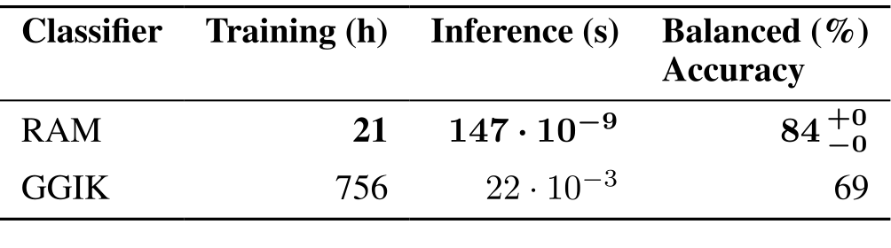
Table 2 reports RAM/GGIK training at 21/756 hours, inference at 147 ns/22 ms and balanced accuracy 84/69%. GGIK’s isolated network query is 83 μs; much remaining time is unbatched input/output processing. These reported H100 timings do not specify a complete single-query synchronization and deployment latency protocol.
The validation/test setup uses thirty million poses across three hundred morphologies; GGIK evaluates only 1% per morphology. Different training sizes, objectives, seed counts and test subsets qualify the comparison. RAM’s test false-positive rate is 25% and increases to 49% near boundaries.
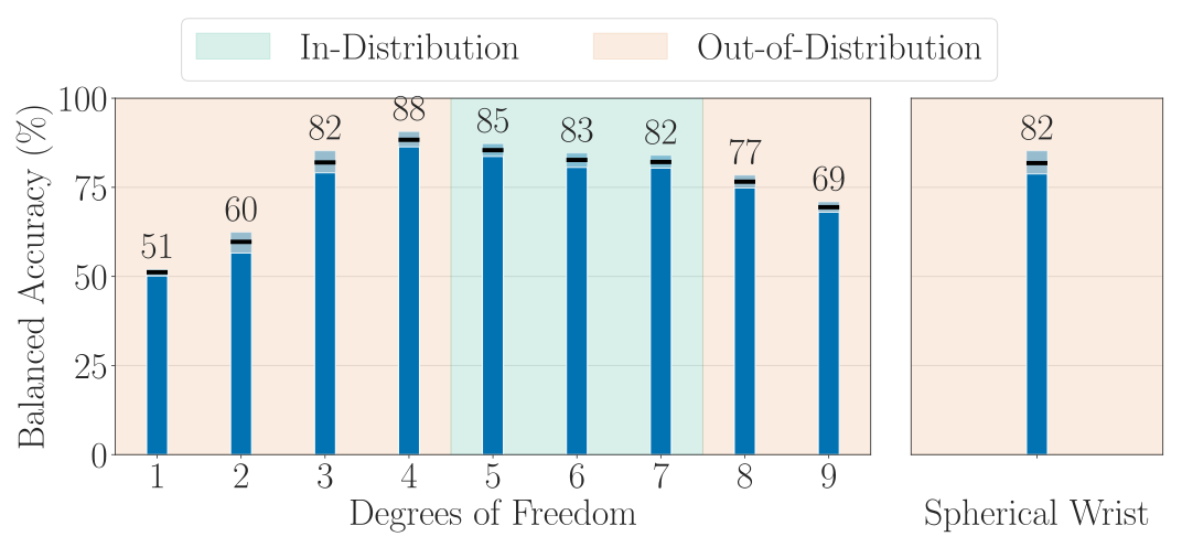
Generalization remains useful on three/four joints and spherical wrists, collapses toward mostly negative predictions on one/two joints, and weakens at eight/nine. Single-morphology comparisons attribute most error to labels, with approximately one point for neural approximation and two for morphology generalization.
5.3 Utility of RAM (RQ3)
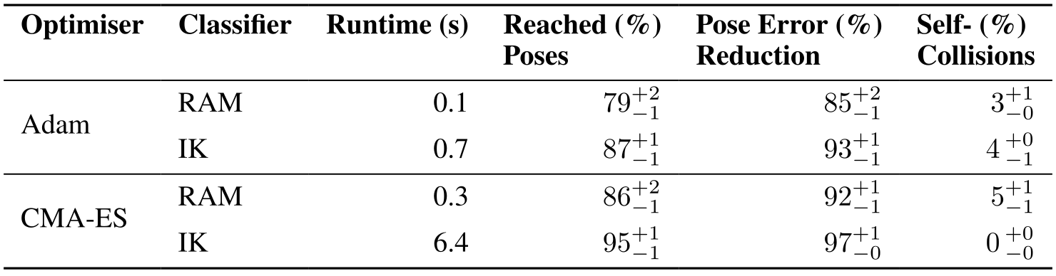
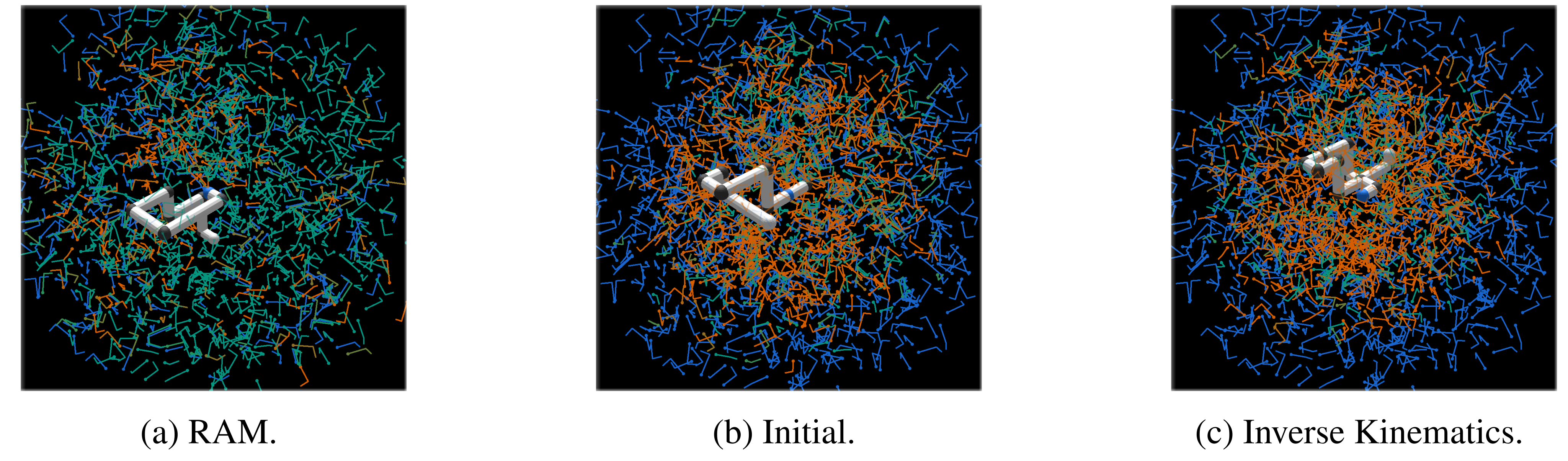
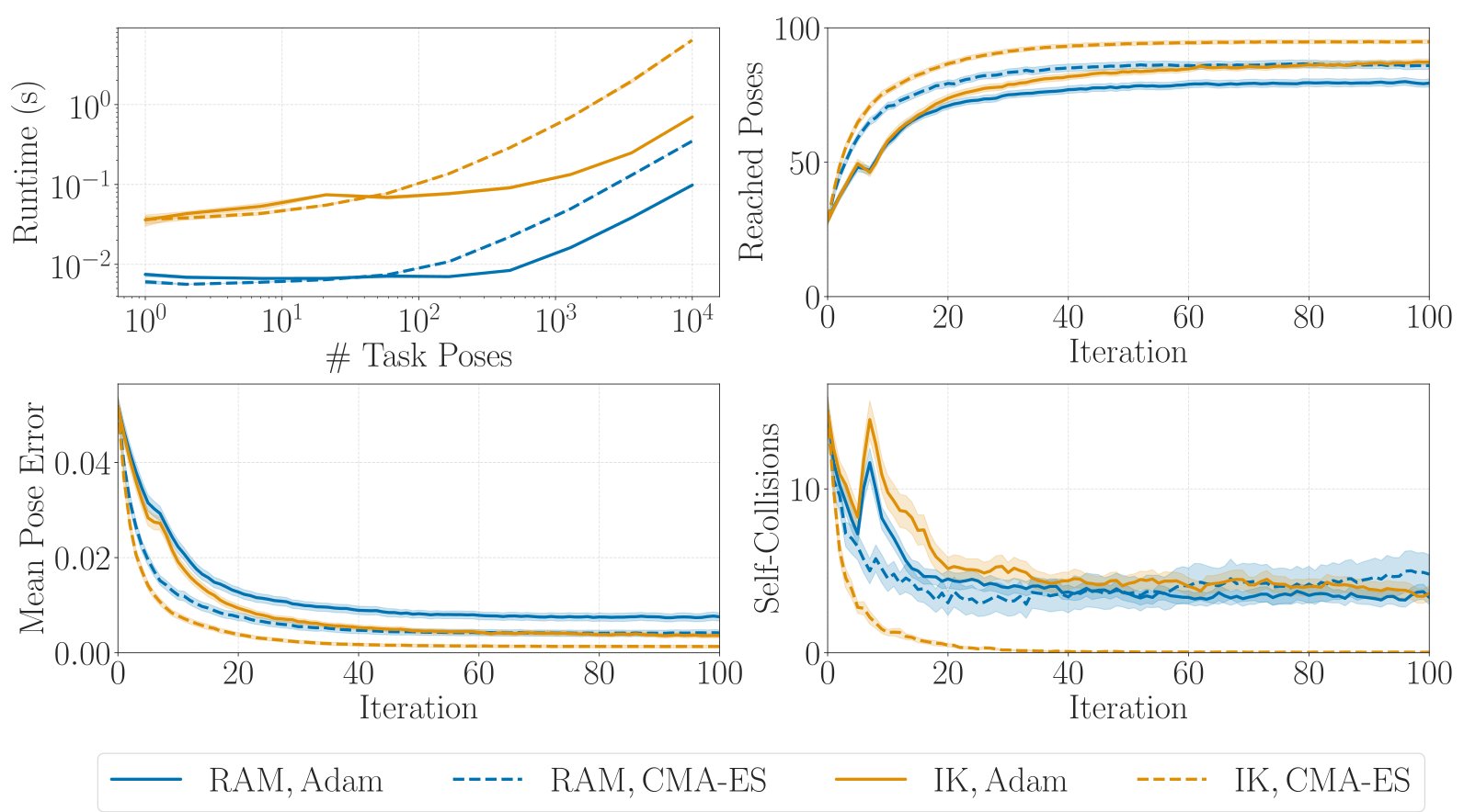
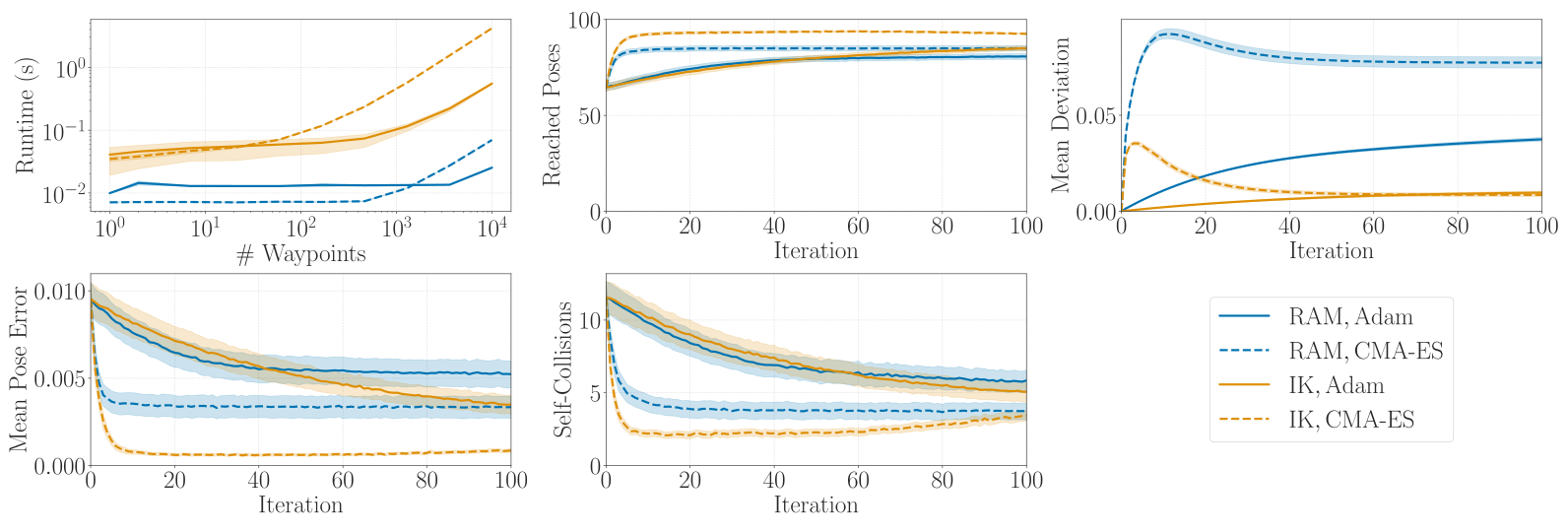
Optimize one thousand six-joint morphologies, each against one hundred targets for one hundred iterations. Only lengths/offsets vary; normalize, zero sub-threshold dimensions and renormalize to avoid inevitable capsule collisions. Compare Adam and CMA-ES with RAM scores versus a smoothed numerical-IK objective.
Morphology optimization takes .1/.7 s for RAM/IK with Adam and .3/6.4 s with CMA-ES: 7×/21× faster. Reached-pose rates fall from 87 to 79% and 95 to 86%; RAM also reduces pose error less. Its Adam self-collision rate is slightly lower, but CMA-ES is worse.
For one thousand trajectories, optimize one hundred pose waypoints using six-dimensional offsets mapped back to valid poses, regularizing deviation from a nominal geodesic. RAM gives 22×/60× speedups, with reached-pose rates 81 versus 85% and 85 versus 93%, and larger deviations. Per-waypoint reachability does not establish a continuous, dynamically feasible, obstacle-free joint trajectory.
6 Conclusion, Limitations, and Future Work
Decoupling reachability from solving inverse kinematics makes a useful fast surrogate, with accuracy and downstream quality bounded by its labels and training family. Training uses five-to-seven-joint serial capsule chains; useful out-of-distribution results extend to some three/four-joint cases.
The model omits environmental collisions, arbitrary topologies and varying link geometry/radii. Better labels, radius conditioning, obstacle inputs, graph encoders and joint morphology/trajectory optimization are proposed directions rather than demonstrated capabilities.
Acknowledgments
The authors acknowledge German Research Foundation and DASHH funding, Leibniz Supercomputing Centre resources, and Olivia Garland’s video and advisory contributions.
Appendix A Preliminaries
Homogeneous transforms encode poses; forward kinematics multiplies modified Denavit–Hartenberg link transforms. Equations retain the complete matrix entries. Evaluate pose error with weighted translation and geodesic rotation, using weights 1/8 and 1/(2π²) and tolerance 10⁻⁴.
The product metric treats translation and rotation independently. Its exponential map adds translation and right-multiplies the rotation; the logarithm returns translation difference and a shortest rotation vector. Interpolation is unique when relative rotation is below π. This chosen metric is not a canonical bi-invariant SE(3) metric.
Equations 4–8
| (4) |
| (5) |
| (6) |
| (7) |
| (8) |
Appendix B Data Synthesis
The supplement specifies hierarchical morphology rejection, uniform reduced-space pose sampling and geometry-derived joint limits used for forward-kinematics labeling.
B.1 Morphology Sampling
Sample link types with both dimensions, length only, offset only or neither. Reject successive zero-length/offset links, constrain twists of co-located joints, and reject long parallel/collinear-axis runs. Sample normalized link-vector magnitudes from exponentials and directions uniformly.
Nonzero capsule dimensions below twice the radius create inevitable scissor contacts and are rejected. Finally test one thousand configurations, rejecting a design if none is both operable and nondegenerate by the stated manipulability check. These finite checks approximate, rather than exhaustively characterize, feasibility.
Equations 9–10
| (9) |
| (10) |
B.2 Pose Sampling
A normalized Gaussian gives a uniform direction; a cube-root uniform radius gives uniform ball volume. Normalize four Gaussian components for a uniform quaternion, convert to rotation and compose the fixed end-effector transform. All sampling formulas remain available.
Equations 11–12
| (11) |
| (12) |
B.3 Label Assignment
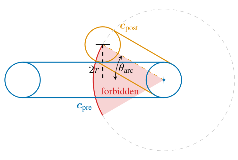
Sample angles uniformly over derived safe arcs. Adjacent capsules can scissor only when both lie in the joint’s rotation plane. The shorter capsule length determines the forbidden half-angle arcsin(2r/lmin); remove that arc around the antiparallel configuration.
Dimensions shorter than twice the radius make this collision unavoidable. End-effector angle stays zero because it has no subsequent joint. These geometric joint limits address the modeled capsule contacts, not arbitrary real-robot joint limits or scene obstacles.
Equations 13
| (13) |
Appendix C Additional Results
The appendix retains complete confusion matrices, boundary and joint-count evaluations, optimization curves, label/encoder ablations and latent-space exploration. True- and false-positive rates are essential for interpreting the balanced-accuracy headline.
C.1 Label Fidelity (RQ1)
As cells become finer, false-positive rates drop 59→34→23→16%, but true-positive rates fall 100→99→97→90% under finite sampling. The selected .040–.042 grid balances these effects; the finest grid is not uniformly better.
C.2 Dataset Generation
The dataset is 204 GB, generated in 360 GPU-hours, with 29% reachable labels. Each morphology contributes one million examples. About 38% admit analytical IK, mostly five-joint designs; for five-joint data, 25% of poses come directly from configurations to supply positives.
Of sampled configurations, 85% are collision-free and 23% of those fill a previously empty cell, about 19% overall. Coverage yield decreases over time. Increasing design count improved generalization within the available compute; a million samples per design was an empirical single-morphology threshold.
C.3 Accuracy of RAM (RQ2)
RAM’s true-positive/false-positive rates are 94/25%, versus GGIK’s 90/61%. RAM inherits occupied-cell dilation and smoothing; GGIK’s loose validation-selected tolerance admits nearby but unreachable targets. Neither matrix makes a positive prediction a reachability guarantee.
C.3.1 Workspace Slices
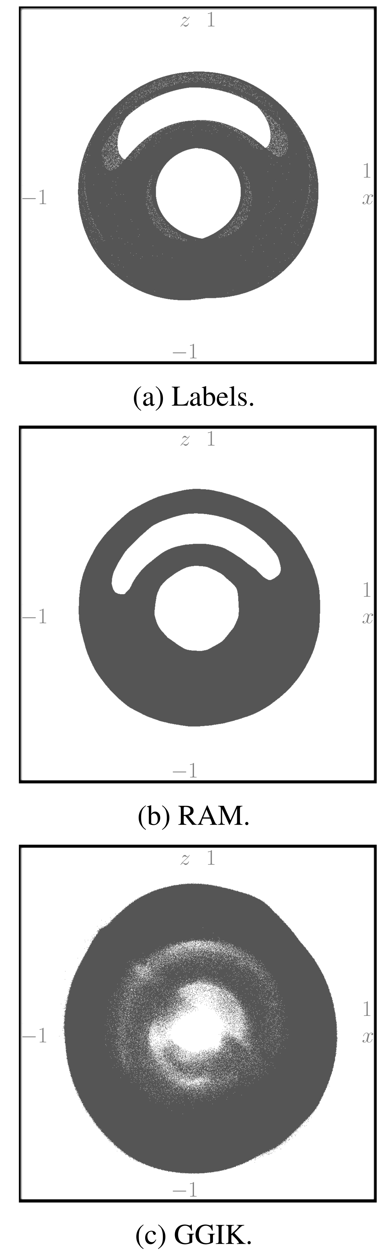
Workspace slices fix orientation and one positional variable and evaluate a million grid points in the first-joint rotation plane. The orientation is chosen from a pose near the estimated workspace center so the slice intersects meaningful structure. These are selected cross-sections, not complete six-dimensional validation.
C.3.2 Boundary Poses
Interpolate between reachable and unreachable pose pairs to target boundaries. Use three hundred morphologies, one thousand pairs each and N=100 geodesic subdivisions; the printed index range includes both endpoints. GGIK again evaluates 1% of samples.
Balanced accuracy becomes 72% for RAM and 62% for GGIK. RAM keeps 94% true positives but false positives rise to 49%; GGIK has 64% true positives and 39% false positives. The methods trade recall and specificity differently near the decision boundary.
Equation 14
| (14) |

C.3.3 Out-of-distribution Generalisation
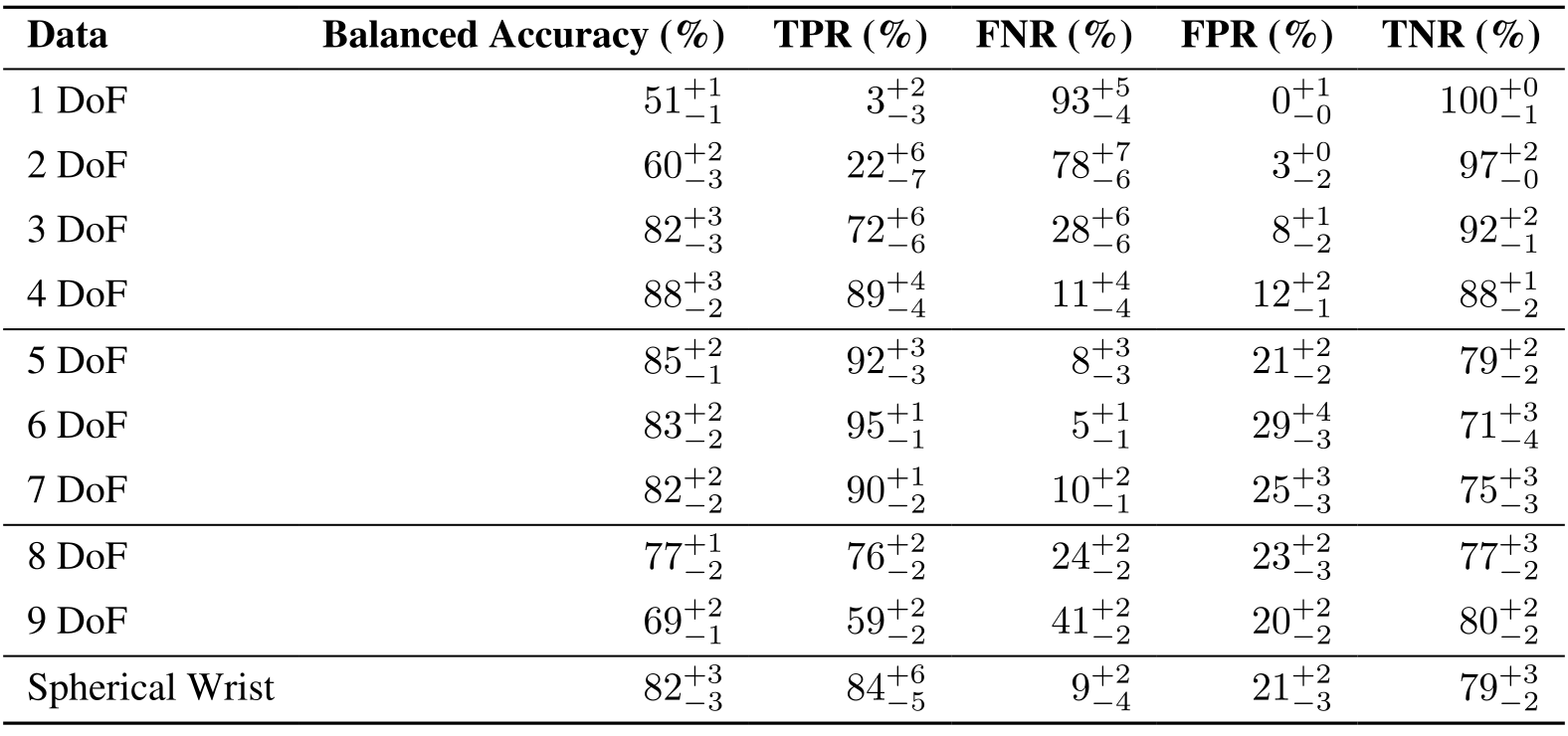
Evaluate one hundred morphologies and one hundred thousand poses per joint-count setting. Balanced accuracy is 51/60/82/88/85/83/82/77/69% for one through nine joints, and 82% for spherical wrists.
Low-joint predictions become conservative; high-joint recall declines gradually. Preserve Table A4’s printed inconsistencies: the one-joint true-positive/false-negative values total 96%, and spherical-wrist values total 93%. They are not silently normalized or treated as exact complementary rates.
C.3.4 Cost of Generalisation
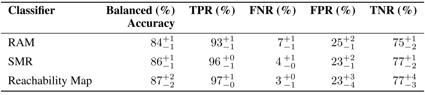
For each of three hundred test designs, compare RAM with a separately trained one-million-example network and a direct reachability-map lookup. Balanced accuracies are 84/86/87%; false positives stay near 25/23/23%.
Generalization mainly lowers true positives, from the map’s 97% to RAM’s 93%. These empirical differences support the label-quality explanation but do not provide an exact causal error decomposition for every morphology.
C.4 Utility of RAM (RQ3)
Both optimization tasks maximize average RAM output; the numerical baseline combines residual pose error, a large collision penalty and, for trajectories, deviation regularization. All original objectives and convergence/runtime plots are retained.
C.4.1 Morphology Optimisation
Optimize mean RAM probability over target poses. The baseline differentiates implicitly through numerical IK, with tolerance 10⁻⁴ and collision-penalty weight 10⁴. Length/offset squashing is ignored in the backward pass, so gradients are approximate near its threshold.
There is a notation conflict: the opening definition makes c true when collision-free, but the printed optimization objective adds +λc while calling it a collision penalty. The intended penalty interpretation is described; the original equations are preserved without inventing a sign correction.
Equations 15–16
| (15) |
| (16) |
C.4.2 Trajectory Optimisation
Optimize tangent offsets and map them to each nominal waypoint. Deviation weight is 1/20, with the same tolerance/collision coefficient as morphology optimization. The metric counts pose differences, not joint-space smoothness or dynamic effort.
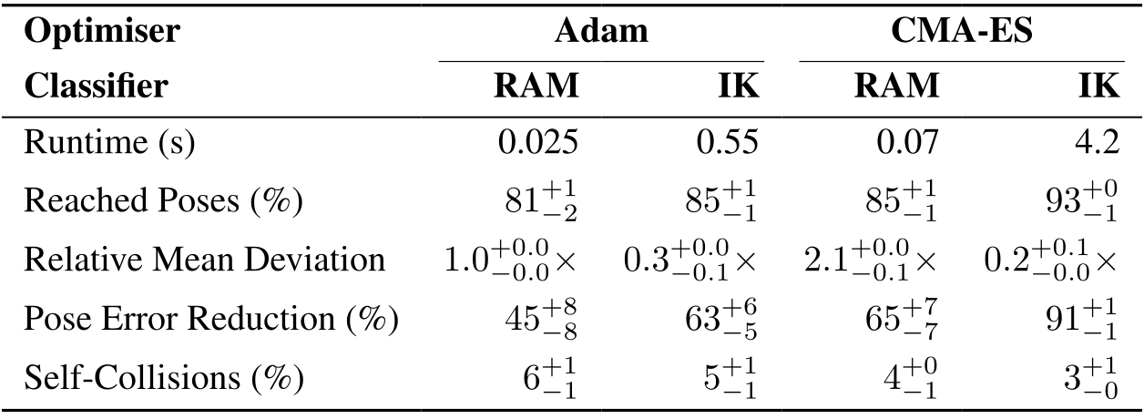
RAM/IK Adam runtime is .025/.55 s and CMA-ES .07/4.2 s. Pose-error reduction is 45/63% and 65/91%; self-collision rates are 6/5% and 4/3%. Relative mean deviations are 1.0/.3 and 2.1/.2, respectively. Speedups therefore come with measurable solution-quality costs.
Equations 17–18
| (17) |
| (18) | ||||
C.5 Ablations
Ablations separate training-label granularity from the morphology encoder choice while keeping the core prediction task and test set fixed.
C.5.1 Impact of the Discretisation Granularity on RAM
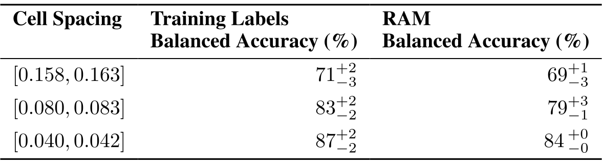
Train ten seeds on each of three equally sized datasets. Label balanced accuracy of 71/83/87% yields RAM accuracy 69/79/84%. The two-to-four-point gap tracks label fidelity, supporting better data as a priority.
C.5.2 Encoder Architecture
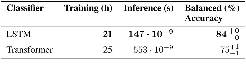
Replace the LSTM with a Transformer without separately tuning it. LSTM/Transformer results are 84/75% balanced accuracy, 147/553 ns reported inference and 21/25 training hours. This supports the tested short-sequence configuration, not a universal architectural ranking.
C.6 Latent Space Exploration
For three thousand designs, select each attribute’s most-correlated latent principal component. Joint count correlates .87 and reachable fraction .65; the former is directly available through sequence length. Reported Fisher-z intervals and p-values do not describe a separate held-out component-selection procedure.
For 150 designs, compare pairwise latent distances with standardized kinematic distances and Monte Carlo workspace Jaccard distances. Mantel correlations are .38 and .49, with permutation significance and bootstrap intervals. This suggests partial functional organization rather than a complete workspace metric or causal disentanglement.
Figure A5 panels c/d show parameter/workspace relationships respectively; the caption’s final parenthetical reverses their order. The plots and labels are retained unchanged.
| Attribute | SCC (%) | -value |
|---|---|---|
| DoF | 0.001 | |
| Moveable Length | 0.001 | |
| Base Twist | 0.001 | |
| Base Length | 0.001 | |
| Base Offset | 0.001 | |
| First Twist | 0.001 | |
| First Length | 0.001 | |
| First Offset | 0.001 | |
| EEF Twist | 0.001 | |
| EEF Length | 0.001 | |
| EEF Offset | 0.001 | |
| Reachability | 0.001 | |
| Centre X | 0.001 | |
| Centre Y | 0.001 | |
| Centre Z | 0.001 | |
| Centre Magnitude | 0.001 | |
| Min. Link Length | 0.001 | |
| Max. Link Length | 0.001 | |
| Std. Link Length | 0.001 | |
| Fraction Type 0 | 0.001 | |
| Fraction Type 1 | 0.001 | |
| Fraction Type 2 | 0.001 | |
| Fraction Type 3 | 0.001 | |
| Max. Pos. Type 3 | 0.001 | |
| Mantel test | ||
| vs. | 0.001 | |
| vs. | 0.001 |
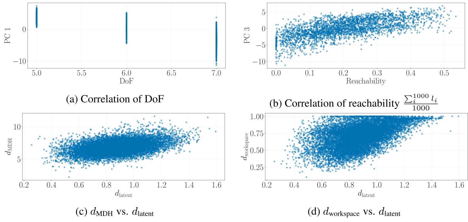
Selectable original panel labels
(a) Correlation of DoF
(b) Correlation of reachability
(c) vs.
(d) vs.
Appendix D Hyperparameters
The selected configuration uses a one-layer, 128-dimensional LSTM and an eight-layer MLP with width 1,792. Train one epoch with batch size 1,000, Adam at 3×10⁻⁴ and β=(.9,.999). Optuna tuning uses a fraction of the training set; all printed hyperparameters remain in Table A10.
| Parameter | Value |
|---|---|
| LSTM latent embedding size | |
| LSTM # layers | |
| MLP hidden layer size | |
| MLP # layers | |
| Epochs | |
| Batch size | |
| Optimiser | Adam [Kingma and Ba, 2015] |
| Learning rate | |