Overview
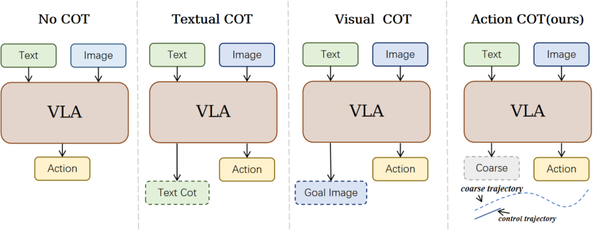
Coarse-to-Control learns a short action-space plan before predicting executable robot actions.
At a glance
Coarse-to-Control adds a supervised planning prefix to a vision-language-action policy. Long future trajectories are compressed into coarse relative motions and encoded with the same vocabulary as short executable chunks. The model generates plan tokens first and action tokens second; only the latter control the robot. It reports 97.9% LIBERO success, 83.3% on SimplerEnv-WidowX, and 62.5% across four physical tasks. The strongest physical gains occur on the tested multistage tasks, within small task-specific demonstration and evaluation sets.

1 Introduction
Direct action prediction must infer detailed motion and longer-term intent from the same observation and instruction. The paper proposes an explicit intermediate representation in action space: a coarse future trajectory that conditions finer control. Training supervises both levels from demonstrations using a shared discrete vocabulary and autoregressive objective. This is a learned latent planning prefix rather than an explicit search procedure or an external planner.
2 Related Work
Related work covers action-generating multimodal policies, intermediate reasoning representations, and discrete action tokenization.
Vision-Language-Action Models.
The method builds on pretrained action-generating models, including FAST action tokenization [28]. Its local policies share a PaliGemma-based architecture initialized from a π0-FAST checkpoint, enabling controlled comparisons between direct execution and action-token planning.
Intermediate Reasoning for VLAs.
Text, generated images, spatial descriptions, and action-centered representations have all served as intermediate policy context. Coarse-to-Control specifically uses compressed future motion in the same token vocabulary as executable actions. Its benchmark comparison spans different models; the local ablations provide the clearer evidence for the planning and tokenizer choices.
Action Tokenization.
Existing codecs discretize individual dimensions, frequency coefficients, or learned action chunks. The proposed shared residual-quantization codec extends learned action-token representations such as FASTer [23] to two modes: coarse future intent and immediate execution.
3 Coarse-Action Planning as Chain-of-Thought
The policy factorizes into a plan distribution conditioned on images, language, and robot state, followed by an execution distribution conditioned on that generated plan. Calling this action-token chain of thought refers to the explicit intermediate sequence; it does not mean the model produces a natural-language explanation.
Equations 1–2
| (1) | ||||
| (2) |
3.1 Coarse-Fine Action Joint Tokenization
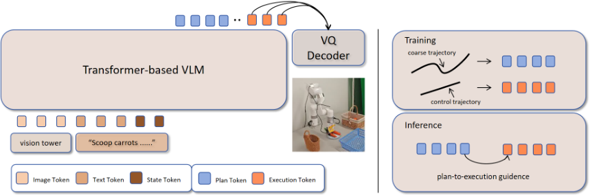
Coarse and executable trajectories are represented by one mode-conditioned action codec.
Action Sub-resolution to Obtain Coarse Action
A longer future window is divided into chunks. Each coarse step sums relative motion within its chunk and keeps the final gripper value. This retains approximate direction and stage transitions while discarding high-frequency detail. The original equations specify the reduction; coarse tokens themselves are not sent to the robot.
Equations 3–4
| (3) | ||||
| (4) |
Dual-granularity Action Tokenizer
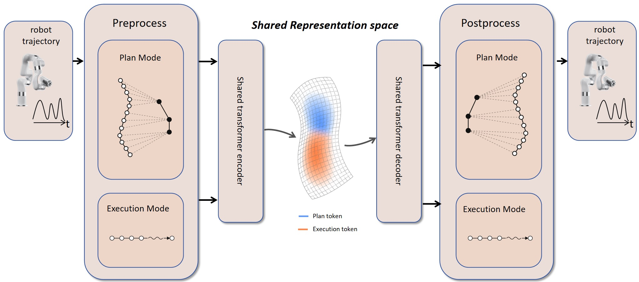
Execution mode encodes short action chunks and planning mode encodes the reduced long future. Shared residual-VQ codebooks and a learned mode condition allow different reconstructions from a common vocabulary. Training combines action reconstruction, codebook, and commitment losses. Sharing code identities encourages compatibility, but does not make coarse and fine token distributions identical.
Equations 5–7
| (5) | ||||
| (6) |
| (7) |
3.2 Plan-Execute Autoregressive VLA
Demonstration-derived plan and execution tokens form one teacher-forced suffix during training. At inference, the policy generates the plan before predicting executable tokens, then decodes only the execution branch. This introduces a prediction dependency: errors in the generated plan can influence the subsequent action distribution, even though both stages are trained jointly at the policy level.
Equations 8–9
| (8) |
| (9) |
4 Experiments
Experiments compare simulation success, physical task completion, planning horizon, tokenizer sharing, and runtime under different intermediate representations.
4.1 Simulation Experiments
Simulation evaluation covers both the LIBERO suites and real-data-to-simulation transfer on WidowX tasks.
Benchmarks and Datasets.
LIBERO [22] uses fifty trials per task across Spatial, Object, Goal, and Long suites. SimplerEnv-WidowX uses twenty-four trials for each of four tasks after training on Bridge demonstrations. The settings use different action horizons and camera configurations.
Baselines.
The tables group prior models by their intermediate representations. These models differ in architecture and training data, so their ranking alone does not isolate reasoning medium. Shared-backbone planning and tokenizer ablations address that issue more directly.
Results.
Coarse-to-Control reaches 97.9% average LIBERO success, including 95.0% on Long, compared with 97.1% and 94.5% for the listed OpenVLA-OFT. On WidowX it achieves 100.0%, 95.8%, 79.2%, and 58.3% across the four tasks, averaging 83.3%; eggplant placement is weaker than several baselines. Table 2’s π0 displayed overall value is inconsistent with its four task entries, so the original values are preserved without recomputing a definitive baseline score.
| CoT Type | Method | Spatial | Object | Goal | Long | Overall |
|---|---|---|---|---|---|---|
| No CoT | -FAST [28] | 96.4 | 96.8 | 88.6 | 60.2 | 85.5 |
| SmolVLA [31] | 93.0 | 94.0 | 91.0 | 77.0 | 88.8 | |
| GR00T-N1 [25] | 94.4 | 97.6 | 93.0 | 90.6 | 93.9 | |
| [3] | 96.8 | 98.8 | 95.8 | 85.2 | 94.2 | |
| OpenVLA-OFT [15] | 97.6 | 98.4 | 97.9 | 94.5 | 97.1 | |
| Textual CoT | ThinkAct [11] | 88.3 | 91.4 | 87.1 | 70.9 | 84.4 |
| [2] | 98.8 | 98.2 | 98.0 | 92.4 | 96.8 | |
| Visual CoT | CoT-VLA-7B [39] | 87.5 | 91.6 | 87.6 | 69.0 | 81.1 |
| WorldVLA [6] | 87.6 | 96.2 | 83.4 | 60.0 | 81.8 | |
| DreamVLA [38] | 97.5 | 94.0 | 89.5 | 89.5 | 92.6 | |
| UniVLA [36] | 95.4 | 98.8 | 93.6 | 94.0 | 95.5 | |
| F1 [24] | 98.2 | 97.8 | 95.4 | 91.3 | 95.7 | |
| UD-VLA [7] | 94.1 | 95.7 | 91.2 | 89.6 | 92.7 | |
| Action CoT | MolmoAct-7B-D [18] | 87.0 | 95.4 | 87.6 | 77.2 | 86.6 |
| Coarse-to-Control (ours) | 98.8 | 100.0 | 97.8 | 95.0 | 97.9 |
| CoT Type | Method | Put Spoon | Put Carrot | Stack Block | Put Eggplant | Overall |
|---|---|---|---|---|---|---|
| No CoT | OpenVLA [16] | 0.0 | 0.0 | 0.0 | 4.1 | 1.0 |
| Octo [27] | 47.2 | 9.7 | 4.2 | 56.9 | 29.5 | |
| [3] | 29.1 | 0.0 | 16.7 | 62.5 | 40.1 | |
| CogACT [20] | 71.7 | 50.8 | 15.0 | 67.5 | 51.3 | |
| Textual CoT | ThinkAct [11] | 58.3 | 37.5 | 8.7 | 70.8 | 43.8 |
| Visual CoT | F1 [24] | 50.0 | 70.8 | 50.0 | 66.7 | 59.4 |
| UD-VLA [7] | 58.3 | 62.5 | 54.1 | 75.0 | 62.5 | |
| Action CoT | Coarse-to-Control (ours) | 100.0 | 95.8 | 79.2 | 58.3 | 83.3 |
4.2 Real-World Experiments
The physical study tests one short placement task and three multistage tasks under shared demonstration and evaluation budgets.
Real-World Setup.
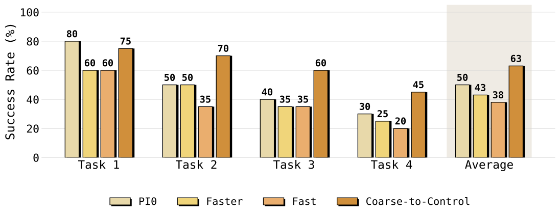
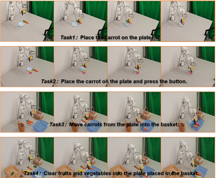
Each task provides fifty demonstrations, and each method receives twenty evaluation trials. Tasks are carrot placement, carrot placement followed by button pressing, moving carrots from a plate into a basket, and clearing produce into a plate placed in a basket. Methods use the same scene setups and success criteria.
Results.
Planning achieves 75%, 70%, 60%, and 45% final success, respectively: fifty successful episodes among eighty trials, or 62.5%. π0 leads the simplest carrot task at 80%, while planning leads the other three. These results support improved completion in the tested sequences, without establishing general robustness across unseen physical environments.
4.3 Analysis
The analysis separates future horizon, representation diagnostics, shared tokenization, and multistage physical progress.
How Does Planning Horizon Matter?
With a fixed joint tokenizer, increasing the planning source horizon from zero to forty to 160 steps raises LIBERO average success from 96.45% to 97.55% to 97.90%. Long-suite success stays 94.20% at forty steps and rises to 95.00% at 160. This supports longer future supervision at the tested settings, with a modest 1.45-percentage-point overall gain over the matched no-plan variant. The separate Faster-AR baseline uses a different tokenizer setup and scores 95.40%.
Why Are Action-Token Plans Effective?
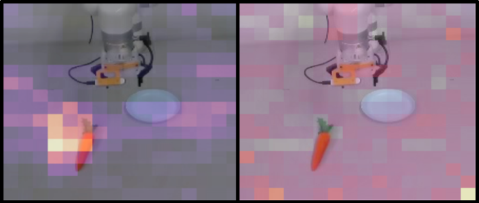
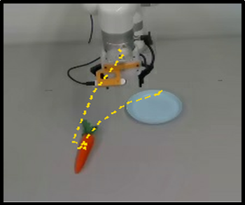
Attention maps and decoded plans suggest that the prefix focuses on relevant objects and encodes motion toward the target. These are qualitative diagnostics, not a causal proof of how attention produces success. Figure 5 retains both the attention comparison and the decoded coarse trajectory.
| Spatial | Object | Goal | Long | Overall | |
|---|---|---|---|---|---|
| 0 | 97.00 | 99.60 | 95.00 | 94.20 | 96.45 |
| 40 | 98.60 | 99.60 | 97.80 | 94.20 | 97.55 |
| 160 | 98.80 | 100.00 | 97.80 | 95.00 | 97.90 |
Should Planning and Execution Share Tokens?
Independent plan/execution codecs score 96.60% overall and 91.60% on Long, while the joint codec reaches 97.90% and 95.00%. Explicit planning therefore helps even without shared codebooks, and sharing adds a further gain. The proposed explanation is reduced translation between token spaces; the experiments support performance differences more directly than that internal mechanism.
| Tokenizer | Spatial | Object | Goal | Long | Overall |
|---|---|---|---|---|---|
| Faster-AR | 99.40 | 98.80 | 94.80 | 88.60 | 95.40 |
| Separate | 97.40 | 99.60 | 97.80 | 91.60 | 96.60 |
| Joint-mode (ours) | 98.80 | 100.00 | 97.80 | 95.00 | 97.90 |
Does Planning Improve Real-World Long-Horizon Performance?
Across the three multistage physical tasks, planning averages 58.3% final success and retains more intermediate progress than the tested baselines. A separate narrower-tokenizer transfer probe also shows shorter successful trajectories. Because step counts exclude failed trials, they measure efficiency conditional on success rather than overall expected task cost.
5 Limitations
The authors identify the limited expressiveness of the current coarse-plan representation and incomplete unification of its two granularities as open questions. The evidence also remains bounded by the selected benchmarks and four small physical task sets. More adaptive planning schemes are proposed, rather than evaluated here.
6 Conclusion
A demonstration-supervised action-space prefix improves control when it provides useful longer-term context before fine action generation. The shared codec, horizon ablation, and physical progress measurements support this design in the tested settings, while the inference interface remains one autoregressive policy.
Appendix
The appendices provide additional ablations, full task progress, data mixtures, tokenizer equations, and training/evaluation protocols.
Appendix A Additional Ablations
Additional experiments examine horizon length, vocabulary sharing, runtime, and physical transfer under narrower tokenizer pretraining.
A.1 LIBERO Design Ablations
The LIBERO ablations distinguish how much future motion is summarized from whether the two token streams share a codec.
Planning Horizon.
The forty- and 160-step plans both compress to twenty coarse steps. Thus increasing source horizon changes the future behavior represented without increasing the number of plan steps. The longer horizon improves overall and Long-suite success at these settings.
Joint Tokenizer versus Separate Tokenizers.
Two independent tokenizers preserve the plan-before-execution ordering but separate code identities. The joint codec improves overall success by 1.3 percentage points. Re-encoded samples have plan/execution support-overlap mass around 0.16, indicating some shared code use alongside different marginal distributions; this diagnostic does not show identical semantics for every token.
Runtime Comparison Across Reasoning Media.
A local visual-reasoning baseline uses 256 prefix tokens, versus 42 planning tokens here. Under the same rollout pipeline, average evaluation time per task is 3,884.27 versus 1,325.53 seconds, about a 2.9-fold difference. This is task evaluation time, not per-action inference latency, and the comparison changes both prefix length and representation.
A.2 Real-World Subtask Progress
The full subtask table distinguishes reaching intermediate states from completing the complete goal. Planning reaches 85% first-stage and 70% final success for carrot-plus-button, 70% and 60% for plate-to-basket, and 70%, 55%, and 45% across cleanup stages. The drop between stages remains substantial despite improvements over the baselines. Figure 7 preserves all physical task keyframes.
| Method | Task | Final | Subtask 1 | Subtask 2 | Subtask 3 |
|---|---|---|---|---|---|
| plan | Carrot+Button | 70.0 | 85.0 | 70.0 | – |
| plan | PlateBasket | 60.0 | 70.0 | 60.0 | – |
| plan | Cleanup | 45.0 | 70.0 | 55.0 | 45.0 |
| faster | Carrot+Button | 50.0 | 75.0 | 50.0 | – |
| faster | PlateBasket | 35.0 | 50.0 | 35.0 | – |
| faster | Cleanup | 25.0 | 55.0 | 35.0 | 25.0 |
| Carrot+Button | 50.0 | 80.0 | 50.0 | – | |
| PlateBasket | 40.0 | 60.0 | 40.0 | – | |
| Cleanup | 30.0 | 55.0 | 40.0 | 30.0 | |
| -fast | Carrot+Button | 35.0 | 40.0 | 35.0 | – |
| -fast | PlateBasket | 35.0 | 45.0 | 35.0 | – |
| -fast | Cleanup | 20.0 | 40.0 | 25.0 | 20.0 |
A.3 Libero-Bridge Tokenizer Real-World Transfer
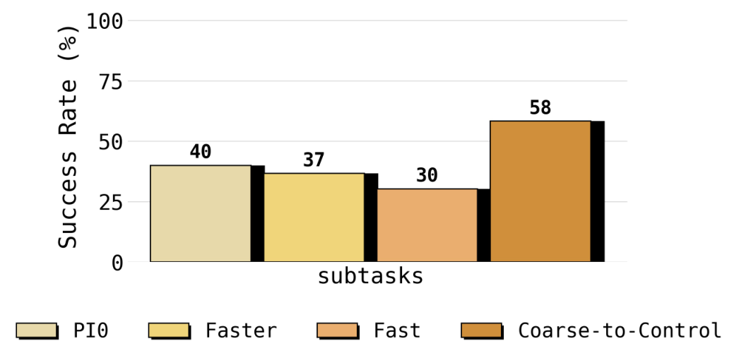
With tokenizers pretrained only on the LIBERO–Bridge mixture, planning and Faster share the same pretraining coverage and downstream physical data. Planning improves carrot success from 40% to 70% and carrot-plus-button from 20% to 35%, with twenty trials per task. Successful rollout length falls from 436 to 239 control steps. This controlled probe supports a planning benefit under domain mismatch, but its success-conditioned duration is not an unconditional speedup.
| Method | Carrot Success | Carrot+Button Success | Avg. Success | Success Steps |
|---|---|---|---|---|
| faster | 40.0 | 20.0 | 30.0 | 436 |
| plan | 70.0 | 35.0 | 52.5 | 239 |
Appendix B Implementation Details
Implementation details specify separate tokenizer pretraining and downstream policy training.
B.1 Dataset Composition
Simulation codecs use LIBERO and Bridge with weights 5:1. The physical codec adds Fractal, Kuka, and DROID end-effector data, each with weight one, alongside Bridge and LIBERO. The codec is frozen for task-specific policy training. This broader physical mixture matters when comparing main results with the narrower transfer probe.
| Setting | Dataset | Weight | Usage |
| Simulation | Libero [22] | 5.0 | Simulation tokenizer |
| Simulation | Bridge [33] | 1.0 | Simulation tokenizer |
| Real world | Fractal [4] | 1.0 | Real-world tokenizer |
| Real world | Kuka [13] | 1.0 | Real-world tokenizer |
| Real world | Bridge [33] | 1.0 | Real-world tokenizer |
| Real world | Droid(EEF) [14] | 1.0 | Real-world tokenizer |
| Real world | Libero [22] | 5.0 | Real-world tokenizer |
Training setup.
Tokenizer pretraining uses eight H200 GPUs. Downstream LIBERO training uses batch size four for 60,000 steps; WidowX uses batch size sixteen for four epochs; physical training uses batch size eight for 30,000 steps. These costs accompany the small per-task demonstration budgets.
| Setting | Training data | Action-token horizon | Policy training |
|---|---|---|---|
| LIBERO | LIBERO demonstrations | 20-step exec / 160-step plan | batch size 4, 60k steps |
| SimplerEnv-WidowX | Bridge demonstrations | 10-step exec / 80-step plan | batch size 16, 4 epochs |
| Real world | Physical robot demonstrations | 20-step exec / 160-step plan | batch size 8, 30k steps |
B.2 Data Preprocessing
Images are resized to 224 pixels and actions/state use 99th-percentile normalization. LIBERO and physical policies use primary and wrist views with a twenty-step execution horizon; WidowX uses ten steps. The pretrained physical codec is reused unchanged during downstream optimization.
B.3 Action Representation
The LIBERO action has seven end-effector dimensions. The main 160-step future is compressed into twenty coarse steps by grouping eight source actions; the forty-step ablation groups two. Relative motions are summed and the final gripper value retained in each group.
B.4 Joint-Mode Action Tokenizer
The shared codec has three residual codebooks with 4,096 entries each. Two temporal patches, seven action dimensions, and three residual levels produce 42 tokens per branch for the twenty-step setting. Latent and mode-conditioning dimensions are 64. Reconstruction uses an action-space L1 loss plus quantization losses, and the commitment coefficient is 0.25.
Equations 10–13
| (10) | ||||
| (11) |
| (12) | ||||
| (13) |
Joint Tokenizer Schematic.
Figure 8 and the retained equations specify mode-dependent action preparation, shared patch preprocessing, decoding, and residual codebook/commitment objectives with stop-gradient operations. Planning and execution samples are drawn equally during codec training. This preserves a shared vocabulary while allowing mode-dependent reconstructions.
Equations 14–19
| (14) | ||||
| (15) |
| (16) |
| (17) | ||||
| (18) |
| (19) |
B.5 Separate-Tokenizer Ablation
The separate-codec ablation keeps the policy’s plan-first generation but trains independent quantizers for the two branches. It tests shared tokenization beyond the effect of adding a planning prefix.
Appendix C Training and Evaluation Details
The training appendix details the policy architecture, optimizer, and simulation evaluation schedule.
C.1 VLA Policy Training
The backbone uses PaliGemma-3B, a SigLIP visual encoder, and a multimodal projector. Images, instruction, and proprioception precede a teacher-forced plan/execution suffix. Deployment generates both stages but decodes only executable tokens into robot actions.
C.2 Optimization
Training uses AdamW at 2.5 × 10⁻⁵, cosine decay, 1,000 warmup steps, and weight decay 10⁻¹⁰. LIBERO runs for up to 60,000 steps; the physical setup uses its specified 30,000-step budget.
C.3 Model Configuration
All local variants start from π0-FAST and share the PaliGemma-based action architecture. The configuration has eighteen layers, eight attention heads, one key–value head, and an 8,192-position limit. Low-rank adaptation is disabled, and exponential-moving-average weights are used for evaluation.
C.4 LIBERO Evaluation
All four LIBERO suites receive fifty trials per task. Controlled comparisons report suite success and total evaluation time. No separate inference-latency measurement should be inferred from those rollout totals.
C.5 SimplerEnv-WidowX Evaluation
WidowX uses Bridge training, one primary camera, a ten-step executable horizon, and an eighty-step source plan reduced to ten coarse steps. It trains for four epochs and replans every ten control steps. Each task receives twenty-four evaluation trials with moving-average weights.
Appendix D Real-World Evaluation Protocol
Each physical task uses fifty demonstrations and twenty trials per method. The last three tasks are multistage and receive intermediate-progress annotations in addition to the binary complete-goal outcome.
Success criteria.
Final success requires completing the entire language goal. An intermediate stage can count as successful even when a later stage fails before timeout. The final and subtask percentages therefore answer different questions and are retained separately.