Overview
This edition follows the complete thirty-three-page, 12 October 2026 v3, including all eight figures, ten numbered tables, thirty-nine numbered equations, three additional displayed equations and 46 references.
At a glance
TAM learns a torque correction between an existing controller and a robot with different dynamics. A long-history encoder infers a latent context; a fast adaptor combines it with current commands and recent motion. Analytic simulator labels train the module without downstream task demonstrations. One Panda model improves several real manipulation policies; transfer to other robot types is demonstrated in simulation. Torque access, a usable ideal model and sufficient actuator authority remain necessary.
1 Introduction
Dynamics mismatch can invalidate a policy even when its observations and goals remain appropriate. Randomizing policy training or identifying physical parameters addresses this problem, but can tie adaptation to a particular policy or require an identifiable parameterization. TAM instead modifies the common torque interface below independently authored policies and controllers.
Random motion histories train a task-independent local correction, reused under RL pushing, behavior-cloned flipping, MPC ball balancing and trajectory tracking. This modularity does not remove the need for coverage of relevant states, loads and actuator behavior.
Related Work.
Appendix A compares dynamics randomization, rapid motor adaptation, identification, adaptive control and residual learning. The central distinction is where adaptation operates and how its correction is supervised.
2 Problem Definition and Scope
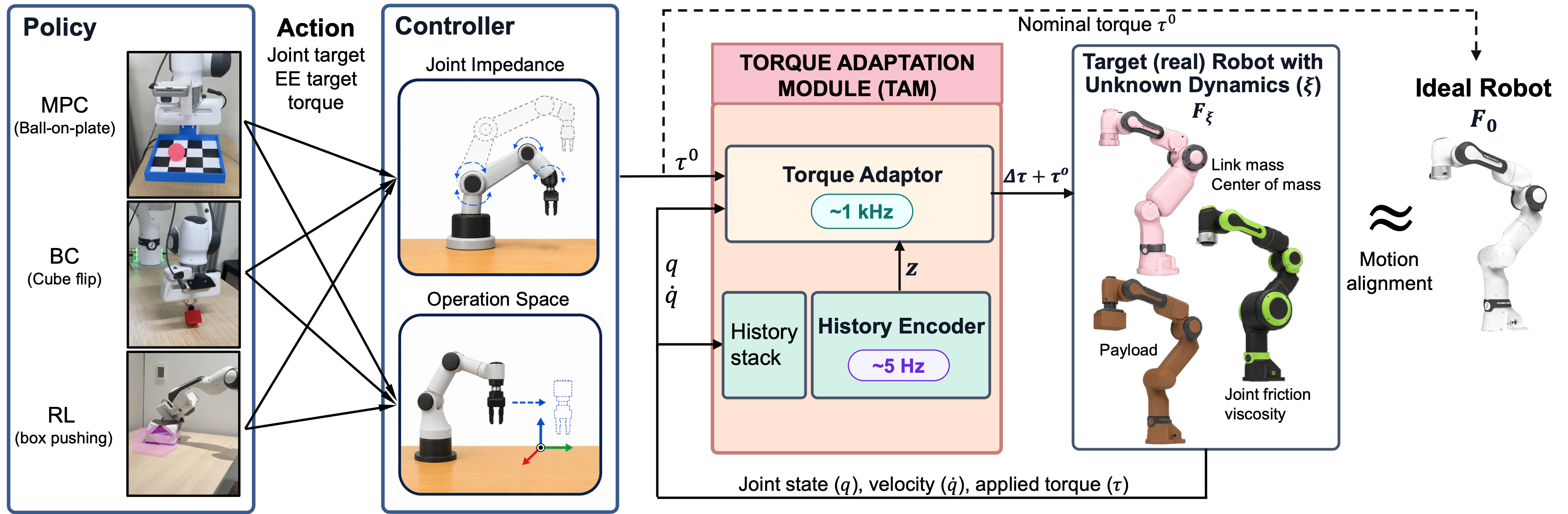
An opaque policy produces actions that a low-level controller converts into nominal joint torques. TAM adds a residual and clips the resulting command to target actuator limits. Ideal and target dynamics share kinematics and joint ordering; only their dynamics/actuation differ. The objective is to reproduce the ideal local acceleration under the same external generalized torque.
External torque is known only to the simulation label generator, never supplied to TAM at deployment. Inverse command maps provide teacher targets. Torque access, a usable ideal model and an invertible simulated actuator model are required. Saturation leaves residual mismatch; clipping alone establishes neither stability nor safety.
Equations
3 Torque Adaptation Module
Supervised local torque matching separates training from downstream tasks. The architecture separates slow inference of dynamics context from fast correction of the current command.
3.1 Data Generation and Training Objective
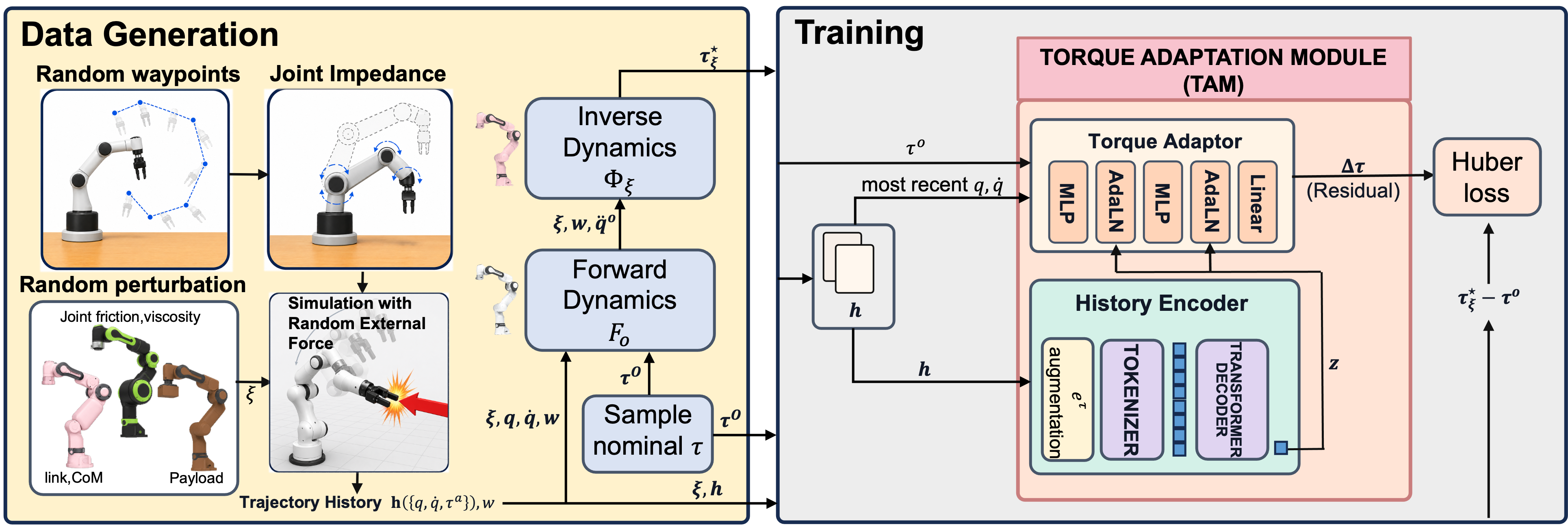
For each recorded joint state and sampled nominal torque, the ideal simulator computes acceleration; the perturbed inverse command map then finds the command producing that acceleration under the same external load. Equation 1 gives this teacher. An elementwise Huber loss compares corrected torque predictions and targets, averaged over joints.
Training covers random waypoint motion rather than task demonstrations. Matching these local transitions can transfer between policies, provided their state, velocity, torque and mismatch regimes are represented; it is not direct optimization of downstream success or long-horizon stability.
Equations 1
| (1) |
3.2 Encoder–Torque Adaptor Architecture
A latent history representation conditions a small torque network. The two modules run at different rates, allowing long context without a Transformer invocation on every hardware tick.
History encoder.
The rolling buffer contains position, velocity and applied-command history over twelve seconds. A physics feature subtracts the ideal inverse-model torque needed for estimated motion from the recorded torque. Its ideal inverse call assumes zero external load, so contact and model mismatch can both affect it; it is not a measured disturbance decomposition.
A patch-based time-series encoder compresses overlapping per-joint windows before causal attention. Earlier informative motion can remain available when recent commands are nearly constant or contact-dominated; finite history still cannot uniquely identify every possible mismatch.
Equations
Torque adaptor.
Per-joint MLPs embed a short local state/torque window. Current nominal torque and the latent context condition the residual prediction through adaptive normalization, following feature-wise conditioning and adaptive layer-normalization designs. Equation 2 retains the exact input timing. The correction is added before final command clipping.
Equation 2
| (2) |
3.3 DAgger Fine-Tuning and TAM Residual-Torque Input
Optional DAgger-style simulation fine-tuning collects histories under TAM’s own corrected commands, reducing training/deployment distribution shift. A further variant feeds previous predicted corrections to the history encoder. This extra residual-command history is distinct from the inverse-model physics feature. Main real experiments use the original model without these refinements.
4 Experimental Results
Multi-robot pretraining uses Panda, Piper, RBY-1, iiwa14 and Flexiv Rizon4. A single Panda-simulation-finetuned model is reused across all physical experiments without DAgger, policy-specific training or real dynamics-calibration trajectories. Real hardware evidence is entirely on Panda; other robot types are simulated.
Trials normally clear history and start the task immediately. TAM passes through nominal torque until its first latent becomes available at about 0.5 seconds; that interval counts toward results. The carried-state tracking condition explicitly preserves a preceding sixteen-second motion history.
4.1 Multiple Policies and Action Spaces
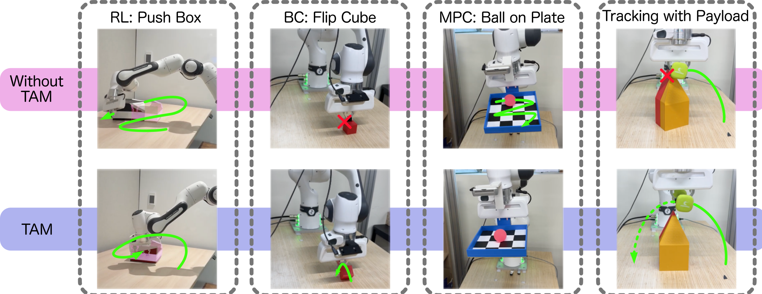
Table 1 reports task-specific outcomes with the same TAM weights. The ideal simulator is a reference, not a universal performance ceiling. Physical success rates have 21 pushing trials and 50 flipping trials; ball balancing has twenty runs. No statistical significance test is reported.

Vision-based pushing policies.
A vision student distilled from a MuJoCo Playground-style state-based policy outputs joint torques. Real pushing succeeds in 10/21 trials directly, 12/21 with Online SysID, 11/21 with RMA, 14/21 with RMA plus TAM and 16/21 with TAM alone. Ideal simulation reports 84%. Adding TAM helps both policies, but combining RMA and TAM is not best here.
Behavior-cloned flip policy.
An ACT policy learns from scripted ideal-simulation flip demonstrations, using gripper-camera RGB and robot state to predict joint targets. Joint impedance converts them to torque before TAM. Success rises from 25/50 directly to 36/50 with TAM; SysID obtains 17/50. The ideal-simulation reference is 73.5%.
MPC ball-on-plate.
A MuJoCo MPC planner uses visual ball-state feedback and iLQR to command torques. Over fifteen seconds, mean goals increase from 8.8 ± 2.4 directly to 13.6 ± 2.9 with TAM; SysID reaches 13.1 ± 2.3 and ideal simulation 15.9 ± 2.3. TAM’s margin over SysID is only 0.5 goal relative to substantial run variation.
4.2 Tracking: Motion Alignment Under Unknown Parameters and Low-Level Controller Switches
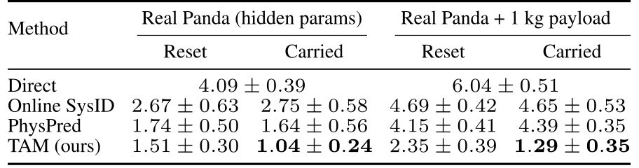
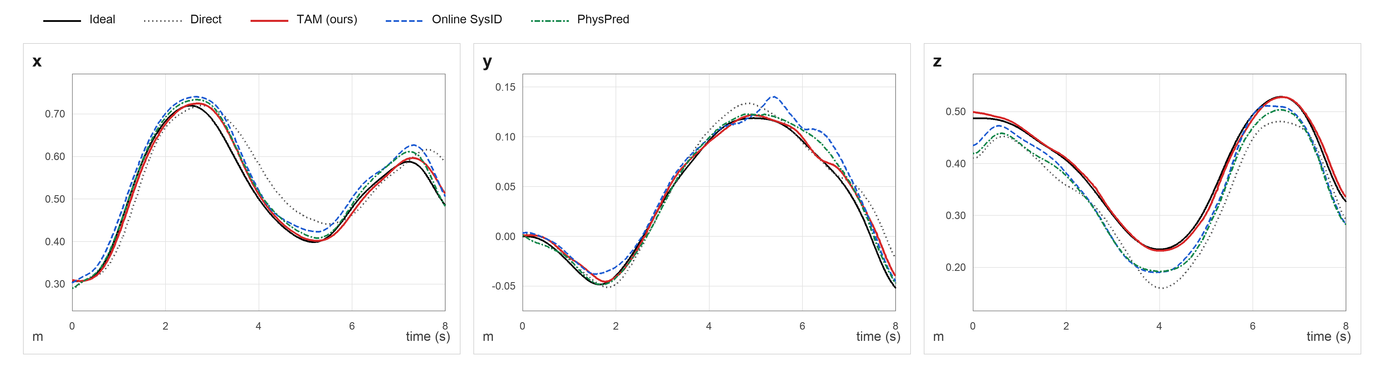
Each real trial tracks sixteen seconds of joint-space motion, then eight seconds with operational-space control. The target segment is scored against its ideal-model reference. Reset clears adaptation at the switch; Carried retains it. Ten trials use the physical Panda, with and without an added 1 kg payload.
TAM’s reset/carried errors are 1.51/1.04 cm without payload and 2.35/1.29 cm with payload, versus Direct 4.09/6.04 cm. It beats the reported SysID and PhysPred cells. Carried results demonstrate reuse of informative prior motion, not cold-start adaptation from the first control tick.
4.3 Simulation Cross-Robot Generalization
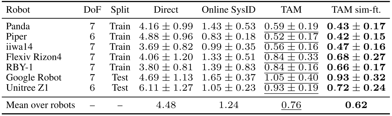
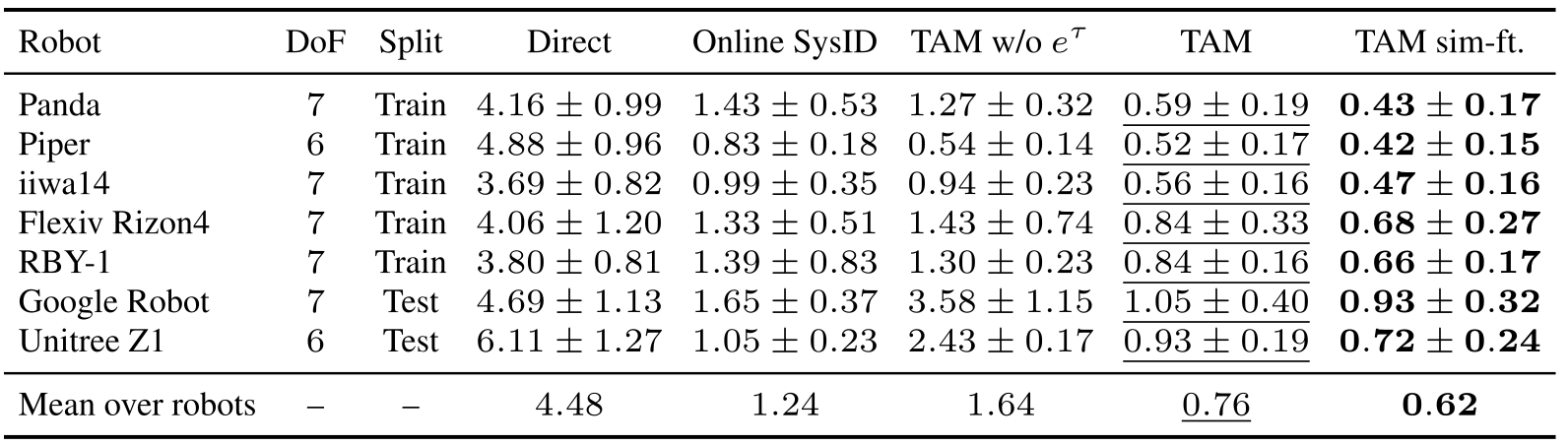
Across seven simulated robots and one hundred randomized trajectories per robot, mean joint RMSE is 4.48° directly, 1.24° with SysID, 0.76° with shared TAM and 0.62° after robot-specific simulation fine-tuning. Shared weights improve both held-out types: Google Robot and Unitree Z1.
The fine-tuned column uses simulation data from each target robot and therefore is not zero-shot transfer. Physical cross-robot deployment is untested, and index-based joint correspondence assumes sufficiently similar serial-arm structure.
4.4 Adaptation Latency Under Abrupt Parameter Changes
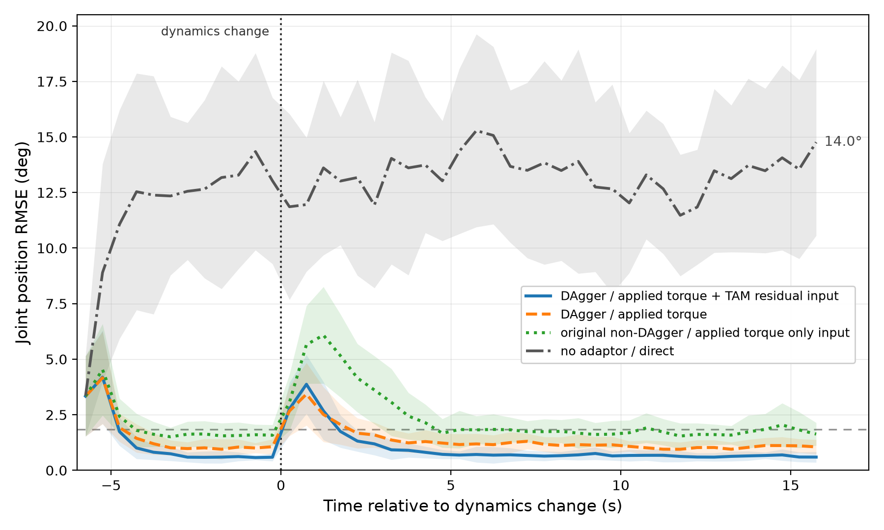
Twenty simulated trajectories undergo an abrupt dynamics change. Recovery to the original model’s 1.83° steady-state threshold takes 4.6 seconds for original TAM and 1.7 seconds for both DAgger variants. Their final errors are 1.10° and 0.64° with added correction history.
Recovery includes catching up with the reference trajectory, not only latent estimation or compute time. Other reported experiments use original TAM. The separate 0.5-second startup result concerns the first latent without an abrupt change.
5 Limitations
TAM needs torque access, matched ideal/target kinematics, a usable ideal inverse model and adequate torque authority. Local supervised correction cannot guarantee long-horizon behavior, collision avoidance or constraint satisfaction. Saturated commands cannot fully compensate a load; unfamiliar contact or actuator behavior can confound history-based inference.
Appendix G gives conditional boundedness for a particular controller form, not a general guarantee for arbitrary policies, impedance controllers or OSC. Position-only interfaces require additional inversion or controller access outside the demonstrated setup.
6 Conclusion
A shared torque-level correction can improve several independently obtained policies without retraining them. The evidence supports this interface on real Panda tasks and simulated cross-robot tracking, with remaining limits from observability, startup delay, saturation, coverage and controller-specific stability conditions.
Acknowledgments
The authors acknowledge Korean IITP/MSIT, NRF, MOTIE/KEIT, InnoCORE and DARIUS support.
Appendix A Related Work
Prior work adapts simulators, policies, physical parameters or action channels. TAM uses simulation-derived local torque labels and a history-conditioned correction shared below downstream controllers.
A.1 Simulator and Actuator Adaptation
Panda identification, BayesSim, active identification and learned actuator/dynamics models can improve model fidelity. TAM instead compresses correction-relevant history without requiring a uniquely identifiable physical parameter vector. Finite excitation and incomplete observations constrain both approaches.
A.2 Policy-Side Adaptation
UPOSI, RMA, manipulator adaptation and long-context policies condition action selection on inferred context. Such context is usually learned together with the policy. TAM places adaptation downstream so existing policy internals and observation interfaces can remain independent.
A.3 Adaptive Control and Online Identification
Classical adaptive control and online parameter estimation exploit structured dynamics and excitation. Their guarantees do not automatically transfer to a learned residual. TAM’s long buffer can reuse earlier informative motion but cannot remove ambiguity between unobserved loads and actuator mismatch.
A.4 Action Transformation and Residual Learning
Grounded action transformation changes the action channel, while residual RL, ASAP and TRANSIC learn corrections with task or real-data supervision. TAM’s distinction is analytic, task-independent torque supervision in simulation and reuse beneath different controllers.
Appendix B TAM Training, Deployment, and Implementation Details
The appendix specifies randomized rollout generation, the invertible actuator model, the two-rate deployment and history preprocessing. All numerical settings are retained in Tables B.1–B.2.
B.1 Simulation Data Generation and Randomization
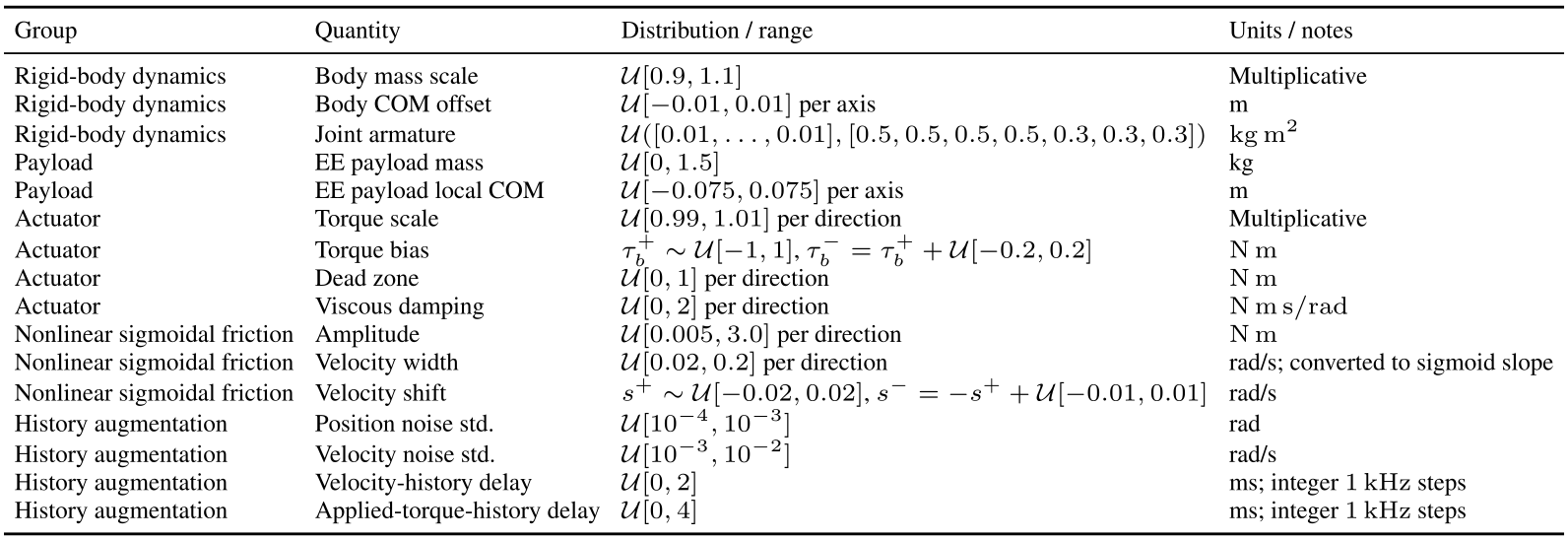
Training varies rigid-body, payload and actuator parameters. Table B.1 is Panda-specific: examples include ±10% body mass, ±1 cm body center of mass, payloads up to 1.5 kg and direction-dependent friction, bias, damping and dead zones. These ranges define the sampled family, not universal robustness bounds.
Rollout generation.
MuJoCo/MJX generates randomized free-space joint-waypoint rollouts under impedance control. Smooth generalized-torque perturbations over finite windows mimic contact effects; they are neither instantaneous impulses nor TAM inputs. The simulator records state, applied and nominal torque, external perturbation, time and sampled parameters.
Original selectable table
| Group | Quantity | Distribution / range | Units / notes |
|---|---|---|---|
| Rigid-body dynamics | Body mass scale | Multiplicative | |
| Rigid-body dynamics | Body COM offset | per axis | m |
| Rigid-body dynamics | Joint armature | ||
| Payload | EE payload mass | kg | |
| Payload | EE payload local COM | per axis | m |
| Actuator | Torque scale | per direction | Multiplicative |
| Actuator | Torque bias | , | |
| Actuator | Dead zone | per direction | |
| Actuator | Viscous damping | per direction | |
| Nonlinear sigmoidal friction | Amplitude | per direction | |
| Nonlinear sigmoidal friction | Velocity width | per direction | rad/s; converted to sigmoid slope |
| Nonlinear sigmoidal friction | Velocity shift | , | rad/s |
| History augmentation | Position noise std. | rad | |
| History augmentation | Velocity noise std. | rad/s | |
| History augmentation | Velocity-history delay | ms; integer steps | |
| History augmentation | Applied-torque-history delay | ms; integer steps |
Actuator perturbation model.
Equations B.1–B.8 define direction-dependent scaling, bias, damping, shifted sigmoid friction and a softened dead zone. A nonzero inner slope makes the dead-zone map invertible. The inverse first removes additive effects, then reverses the dead zone and torque scale.
Notation needs care: main Section 2 defines recorded τᵃ as the clipped command, whereas B.5 uses the same symbol for actuator-transformed effective torque. Command history and physical actuator output are distinct quantities; the printed equations are retained without inferring undocumented implementation behavior.
Equations B.1–B.8
| (B.1) |
| (B.2) |
| (B.3) | ||||
| (B.4) |
| (B.5) |
| (B.6) |
| (B.7) |
| (B.8) |
Nominal torque query sampling.
Teacher queries add predefined Gaussian noise around each recorded rollout torque and clip to the training range. They are not commands generated by the downstream task policies. Sixty-four nominal samples per recorded state broaden local command supervision.
Equation B.9
| (B.9) |
B.2 Deployment Details
A workstation GPU updates history context asynchronously at 5 Hz for Panda. The controller-side CPU applies the fast adaptor at 1 kHz, reusing the latest latent between updates. No external-torque estimate enters TAM. After reset, missing history is zeroed/masked and nominal torque passes through until enough samples arrive, typically 0.5 seconds; a full twelve-second buffer is unnecessary.
External torque and payload identifiability.
A filtered external-torque estimate can reveal payload or rigid-body mismatch while missing some commanded-versus-transmitted actuator effects. With both payload and actuation unknown, their contributions need not separate uniquely. TAM predicts their combined correction from robot history; neither a payload label nor external-torque measurement is supplied in the reported experiments. Such measurements remain possible future auxiliary cues.
Deployment runtime footprint.
Panda’s encoder has about 4.4 million parameters and its adaptor 63 thousand. Reported RTX 3080 footprint is 1.29 GB; encoder updates average 0.999 ± 0.045 ms over one hundred runs, while adaptor heads average 0.155 ± 0.002 ms over two hundred. These compute measurements are distinct from the deployed 5 Hz/1 kHz scheduling and closed-loop recovery latency.
B.3 Implementation Details
Table B.2 retains patch size 400, stride 200, five Transformer layers, eight heads, token width 256, latent width 64 and Huber threshold 0.01, alongside filtering, masking and deployment settings.
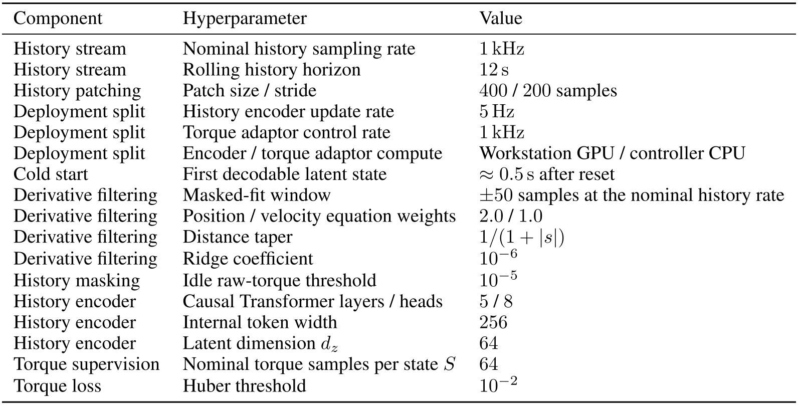
Original selectable table
| Component | Hyperparameter | Value |
|---|---|---|
| History stream | Nominal history sampling rate | |
| History stream | Rolling history horizon | |
| History patching | Patch size / stride | / samples |
| Deployment split | History encoder update rate | |
| Deployment split | Torque adaptor control rate | |
| Deployment split | Encoder / torque adaptor compute | Workstation GPU / controller CPU |
| Cold start | First decodable latent state | after reset |
| Derivative filtering | Masked-fit window | samples at the nominal history rate |
| Derivative filtering | Position / velocity equation weights | / |
| Derivative filtering | Distance taper | |
| Derivative filtering | Ridge coefficient | |
| History masking | Idle raw-torque threshold | |
| History encoder | Causal Transformer layers / heads | / |
| History encoder | Internal token width | |
| History encoder | Latent dimension | |
| Torque supervision | Nominal torque samples per state | |
| Torque loss | Huber threshold |
Patch token construction.
Each patch flattens position, velocity, applied torque and physics residual for one joint. An MLP embeds it, learned joint IDs identify its coordinate, and causal attention uses rotary position encoding. A projection produces the per-joint latent. Equation B.10 preserves the exact patch indexing.
Equation B.10
| (B.10) |
Derivative filtering for the physics residual.
Acceleration comes from a masked local cubic fit jointly using position and velocity equations, with stronger weight on nearby observations and small curvature regularization. The ±50-sample window uses the available recorded history. Invalid/idle rows are masked; insufficient data triggers interpolation or filtered velocity differences, then zero acceleration. The same procedure reconstructs hardware history.
Closed-loop rollout loss and training-time augmentations.
A short closed-loop loss rolls the perturbed simulator under sampled TAM-corrected commands, updates the local window and reapplies teacher supervision. Long-context latents still come from logged history. Training also injects state noise and randomized velocity/torque-history delays to reduce sensitivity to real observation artifacts.
Appendix C Torque Retargeting and Explicit-Parameter Baselines
The analytic inverse map generates training commands and is reused by explicit-parameter baselines. This shared retargeting interface separates parameter estimation quality from the commanded ideal acceleration.
C.1 Inverse Torque-Command Map
Equation C.1 applies rigid-body inverse dynamics, subtracts the known external generalized torque and inverts the modeled actuator effects. Keeping the same external load in ideal forward and target inverse dynamics preserves its intended physical effect instead of silently canceling contact.
That preservation is structural in the simulator teacher, not separately certified for the learned network. Label generation removes simulator torque limits and softens/clips problematic inverse branches; hardware limits are applied later, so some ideal targets may be unreachable.
Equation C.1
| (C.1) |
C.2 Online SysID and PhysPred Baselines
Online SysID uses a particle-filter physical estimate; PhysPred uses a history network to predict explicit parameters, inspired by Dynamics as Prompts. Both replace TAM’s direct latent-to-residual mapping with the same analytic ideal-acceleration retargeting. PhysPred is a controlled baseline here, not a reproduction of every detail of that prior method.
Online SysID parameter estimation.
The filter maintains 512 parameter particles and a fifty-sample buffer, scoring 49 one-step transitions with weighted position/velocity errors. It updates every fifty samples, resamples below half the effective population and adds bounded jitter. GPU MJWarp evaluates candidate dynamics outside the hard real-time torque loop.
It sees the same robot-side signals, ideal model and torque limits as TAM, without rewards or ground-truth parameters. It additionally receives a hand-chosen parameter family, bounds and payload-body index. Non-smooth, multimodal actuator effects motivate a particle filter rather than a local Gaussian approximation.
Equations C.2–C.3
| (C.2) |
| (C.3) |
Shared torque retargeting.
The estimated model inverts the ideal acceleration induced by the current nominal command, with zero external-torque input. The resulting correction is clipped to the same joint limits. This does not eliminate finite-window ambiguity, parameter-family misspecification or insufficient torque authority.
Equations C.4–C.5
| (C.4) |
| (C.5) |
Appendix D Tracking Experiment Details
Table D.1 distinguishes task success from tracking error and separates policy type from the downstream controller. The following protocols explain both carried-state reuse and simulated transfer.

Original selectable table
| Experiment | Policy type | Low-level controller | Metric |
|---|---|---|---|
| Tracking | Reference tracking with unknown parameters | Joint impedance / OSC | Joint or end-effector tracking error |
| Vision pushing | RL policy | Direct torque | Success rate |
| Behavior-cloned flip | BC policy | Joint impedance | Success rate |
| Ball-on-plate | MPC policy | Direct torque | Goals per run |
D.1 Source-to-OSC Evaluation Protocol
All methods share sixteen-second source joint trajectories and eight-second OSC targets. The source uses randomized sinusoidal amplitude, period and phase; the target uses five Cartesian waypoints. The paper reports target-position RMSE, while logging source tracking and terminal error separately.
Reset conditions clear adaptation at the switch; Carried retains it. Figure D.1 plots one carried-state payload trajectory and does not show all trials. Exact gains, waypoint ranges and sampling intervals remain in the original source.
D.2 Cross-Robot Tracking Protocol
Each simulated robot uses its own MuJoCo model and joint defaults. One hundred randomized sixteen-second joint references yield mean ± standard deviation. Shared pretraining excludes Google Robot and Unitree Z1; robot-wise fine-tuning then uses target simulation without new real data.
D.2.1 Cross-Robot TAM Transfer Implementation
Robots use their own joint coordinates and the first N entries of a learned joint-ID table. Per-joint embeddings, attention and adaptor weights are shared; no learned inter-robot joint mapping is added. Target models supply normalization, ideal-model residuals and torque limits.
This assumes roughly comparable ordered serial chains, not semantic joint matching or arbitrary morphology transfer. Different ordering/actuators can degrade performance; more joints than the configured ID table require extension and training.
D.2.2 Cross-Robot Physics-Residual Ablation
Removing the physics residual raises mean simulated joint error from 0.76° to 1.64°. Degradation is particularly large on held-out Google Robot, 1.05°→3.58°, and Unitree Z1, 0.93°→2.43°. Every row worsens, though Piper changes only 0.52°→0.54°. The feature helps within this robot family; it does not establish morphology-independent invariance.
Appendix E Policy Implementation Details
Policy-specific perception and planning remain outside TAM. Their details matter for interpreting the real experiments, especially what “no real calibration” means: no real dynamics-calibration trajectories are used for TAM, while task vision still uses geometric camera/plate calibration.
E.1 Vision-Based Box Pushing
Pushing combines a privileged simulator teacher, a point-cloud student and a separate real object-pose estimator used for state estimation and success measurement.
Policy training.
A PPO teacher observes simulator joint state, end-effector/object poses, goal and previous action. Reward encourages side contact, position/orientation alignment and smooth robot actions. The student is subsequently distilled from this policy rather than trained directly by point-cloud RL.
Point-cloud student.
DAgger matches teacher torques from two randomized depth views. Fused points include camera-source labels, twenty synthetic gripper keypoints and the goal-box mesh. A PointNet-style encoder with mean pooling feeds a recurrent GRU alongside proprioception/goal inputs; an auxiliary box-vertex head encourages object geometry retention.
Real-world box-pose estimation and point-cloud preprocessing.
Calibrated camera transforms project depth into robot coordinates, crop the workspace and remove table points, retaining at most 6,000 points per view. A 256-particle planar box-pose filter scores the known mesh against observed points and discards pose caches older than 0.25 seconds.
Success uses this estimate: within 3 cm and 15° of the target before fifteen seconds. Thus perception accuracy contributes to the task metric; the experiment does not use simulator object state on hardware.
RMA policy-side baseline.
RMA’s privileged teacher context is distilled into a student history estimator inside the pushing policy. TAM instead operates after that policy. The RMA-trained policy is more conservative, with accumulated wrist-orientation change 250.23° versus 334.11°; this supports, without isolating causality, the authors’ explanation for RMA+TAM trailing native-policy TAM.
E.2 Behavior-Cloned Flip Policy
A scripted simulator demonstrator moves to a pre-flip pose, reorients the cube through contact and retracts. Successful episodes train an ACT policy with ResNet-18 visual features, Transformer encoder/decoder and conditional-VAE latent. It predicts chunks of seven absolute joint targets plus gripper actions from RGB and compact robot state.
TAM is added after ACT training at the impedance controller’s torque output. Physical success means the requested cube face ends on the bottom; demonstrations are synthetic, not human teleoperation.
E.3 Ball-on-Plate MPC
MPC runs at 50 Hz with a 20 ms planning timestep and 0.4-second horizon. It inserts measured arm and estimated ball states into the planner and sends the first planned torque through TAM. Goals are sampled at radial distances 2–5 cm; a 5 mm reach radius and 10 mm exit hysteresis determine events over fifteen seconds.
iLQR residual design.
A clipped proportional velocity generates a smooth local ball reference, capped at 0.04 m/s. Six residual groups penalize ball tracking, plate-center displacement, joint posture, velocity limits, torque effort and leaving the plate, with weights 40, 1, 0.1, 5, 0.2 and 1,000. These are soft planning costs, not hard safety guarantees.
Equation E.1
| (E.1) |
Analytical ball-position estimator.
Eight startup images calibrate a checkerboard homography and camera-to-plate transform. Fixed HSV thresholds segment the red ball; a ray intersects the ball-center plane using known radius to recover planar position. Recent estimates yield velocity, and failed detections reuse the last valid position. This is an analytic visual estimator with geometric calibration, not a learned perception model.
Appendix F Additional Analyses and Ablations
Additional experiments examine architecture, latent organization, unnecessary correction on an ideal plant, unseen friction and adaptation timing. They support the tested regimes rather than unrestricted robustness.
F.1 Architecture Ablations
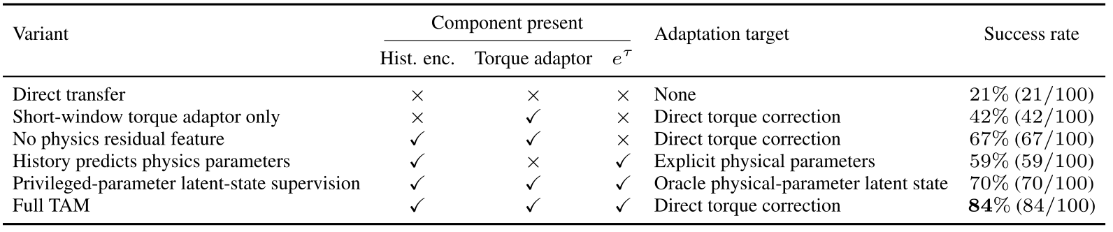
In one hundred simulated pushing trials, success is 21% directly, 42% with only the short-window adaptor, 67% without the physics residual, 59% with explicit parameter prediction, 70% with privileged-latent supervision and 84% for full TAM. The privileged-latent row is an alternative training target, not simply an ablated component. No uncertainty or significance analysis accompanies these success counts.
Original selectable table
| Variant | Component present | Adaptation target | Success rate | ||
|---|---|---|---|---|---|
| Hist. enc. | Torque adaptor | ||||
| Direct transfer | None | () | |||
| Short-window torque adaptor only | Direct torque correction | () | |||
| No physics residual feature | Direct torque correction | () | |||
| History predicts physics parameters | Explicit physical parameters | () | |||
| Privileged-parameter latent-state supervision | Oracle physical-parameter latent state | () | |||
| Full TAM | Direct torque correction | () | |||
F.2 Latent-State Bottleneck Analysis
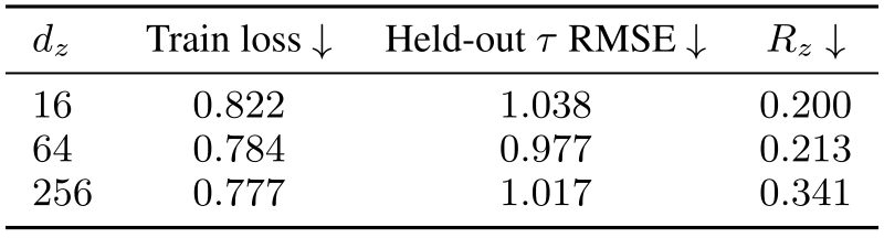
A crossed bank replays 64 fixed trajectories under 64 physical conditions with high-gain tracking, separating motion identity from dynamics. At the same training step, latent dimensions 16/64/256 yield held-out torque RMSE 1.038/0.977/1.017. The selected width 64 is best in this small sweep, not a sharply established global optimum.
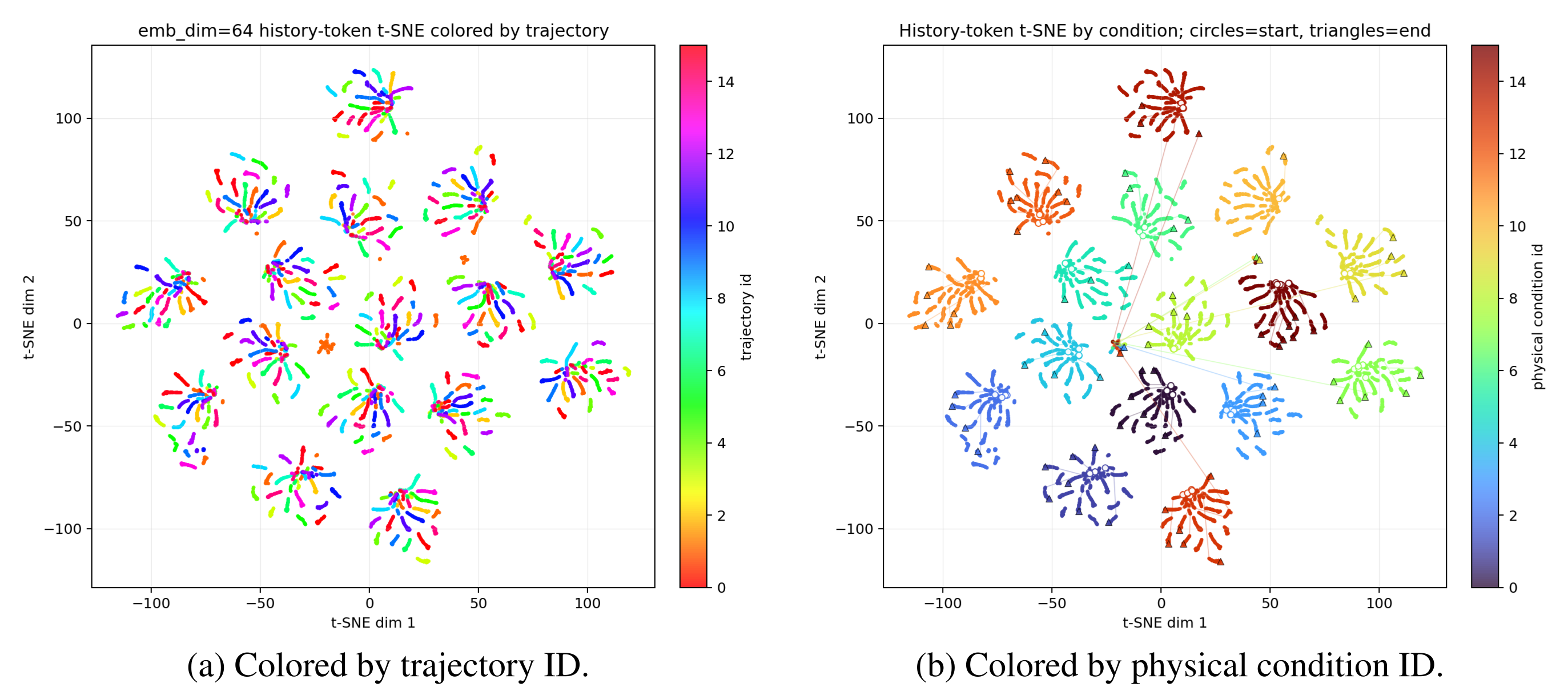
Width 256 lowers training loss but raises the trajectory-to-condition distance ratio from 0.213 to 0.341 relative to width 64. The small 16-versus-64 error gap warrants restraint; t-SNE is supporting visualization rather than proof of complete disentanglement.
Metric computation.
The evaluator encodes the first half of each replay and measures teacher-residual prediction error in the second. Latents are standardized coordinate-wise; normalized distances compare different trajectories under one condition against different conditions on one trajectory. Equations F.1–F.5 retain the teacher and ratio definitions. Lower ratio means stronger condition-based grouping under this controlled replay protocol.
Equations F.1–F.5
| (F.1) |
| (F.2) |
| (F.3) |
| (F.4) |
| (F.5) |
Original selectable table
| Train loss | Held-out RMSE | ||
|---|---|---|---|
F.3 No-Mismatch Check: TAM on the Ideal Robot
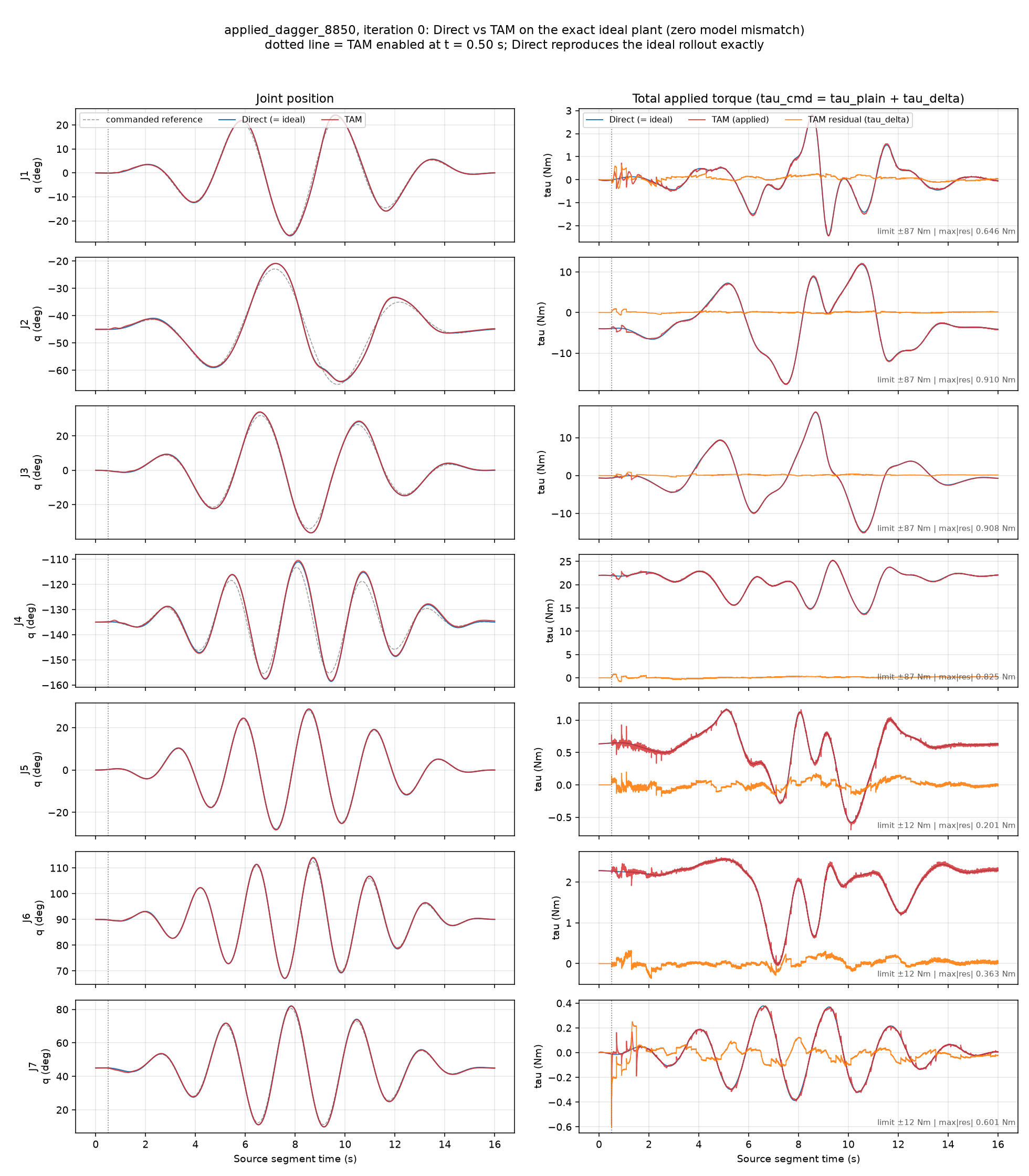
On the exact ideal simulated plant, both Direct and TAM achieve 84/100 pushing successes and 15.9 ball goals per run. TAM introduces small nonzero motion differences: 0.20 ± 0.01° joint RMSE across five trajectories, with peak residual torque below 0.91 Nm. Task-level performance is unchanged in these checks, not exact identity of all motions or a universal non-degradation guarantee.
F.4 Out-of-Distribution Friction Robustness
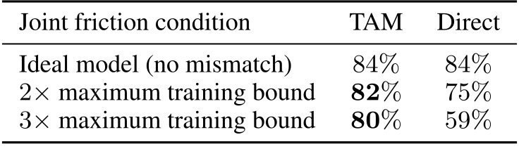
At twice and three times the maximum training friction, simulated pushing success is 82%/80% with TAM versus 75%/59% directly, over one hundred trials per condition. This supports robustness to those friction shifts. Real pushing/flipping also introduce contact patterns absent from random-motion training; neither result covers arbitrary loads, contacts or actuator saturation.
Original selectable table
| Joint friction condition | TAM | Direct |
|---|---|---|
| Ideal model (no mismatch) | ||
| maximum training bound | ||
| maximum training bound |
F.5 Adaptation-Latency Protocol and Warm Start
Startup passes nominal torque unchanged for roughly 0.5 seconds. The source reports a 90% tracking-error reduction after this initial context becomes available without a dynamics jump. In the abrupt-change test, trajectories begin five seconds before the switch; recovery uses the same original-TAM 1.83° threshold for every variant and includes trajectory catch-up.
Appendix G Stability and Oscillation Analysis
The appendix offers a conditional tracking-error bound and a measured oscillation check. Neither establishes general safety or stability for every downstream policy/controller combination.
G.1 Bounded Tracking Errors Under a Bounded Residual
A standard manipulator Lyapunov argument treats the learned correction as a bounded input. Under the stated passivity-form controller, damping dissipates energy quadratically while bounded disturbances inject it at most linearly, yielding a finite error ceiling.
Tracking errors.
Position error e and filtered error s = ė + Λe separate the mechanical dynamics from a stable first-order position-error equation. Λ is symmetric positive definite. This tracking error e is distinct from TAM’s torque-space feature eτ.
Equations G.1–G.2
| (G.1) |
| (G.2) |
Robot dynamics and controller.
The assumed base controller supplies model-based reference acceleration, Coriolis and gravity terms plus damping of s. With a compatible rigid-body model, Ṁ − 2C is skew-symmetric and Equation G.3 follows. A generic PD or OSC controller need not satisfy this form; the proof does not automatically cover every experimental controller.
Equations G.3
| (G.3) |
Bounds and operating conditions.
Assume globally existing unique trajectories, uniformly bounded positive inertia, bounded remaining disturbances and bounded induced additive TAM torque. Final command saturation must be inactive or its discrepancy must have a separately justified bound inside the disturbance. Command clipping alone does not establish these assumptions.
Proposition G.1 bounds filtered, position and velocity errors using initial errors, inertia bounds and the smallest damping/filter eigenvalues. The full statement and formulas are preserved below.
Equations G.4–G.7
| (G.4) |
| (G.5) |
| (G.6) |
| (G.7) |
Step 1: Damping dominates at large error.
Differentiate kinetic-like energy ½sᵀMs. Skew symmetry cancels the inertia/Coriolis cross term, leaving damping plus input work. Cauchy–Schwarz gives negative energy derivative whenever the filtered-error norm exceeds the input bound divided by minimum damping.
Equations G.8–G.10
| (G.8) |
| (G.9) |
| (G.10) |
Step 2: An energy ceiling bounds the filtered error.
The upper inertia bound converts that norm threshold to an energy threshold. Energy cannot cross above both this threshold and its initial value while its derivative is negative. The lower inertia bound then converts the energy ceiling into the stated uniform bound on s.
Equations G.11–G.13
| (G.11) |
| (G.12) |
| (G.13) |
Step 3: Bound position and velocity errors.
Apply the same argument to ½‖e‖² under ė = −Λe + s. Position error is bounded by the larger of its initial norm and the filtered-error bound divided by minimum filter gain. The triangle inequality then bounds velocity error.
Equations G.14–G.16
| (G.14) |
| (G.15) |
| (G.16) |
Interpretation for TAM.
The proposition establishes bounded errors under its assumptions, without a convergence rate or settling time. More permitted residual torque can enlarge the worst-case bound; actual compensation may nevertheless reduce the combined disturbance. The result does not certify collision avoidance, contact-force limits or state constraints.
G.2 Empirical Oscillation Analysis on the Real Panda
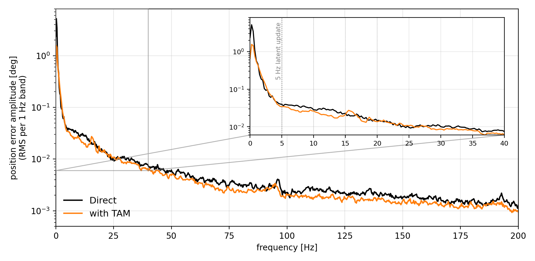
Ten paired real-Panda rollouts compare joint-position-error spectra with and without TAM, aggregated as RMS per 1 Hz band over 0–200 Hz. Figure G.1 shows no dominant new peak, including around the encoder’s 5 Hz update. This empirical check does not rule out oscillation under other trajectories, loads or controllers.