Overview
Code. This edition follows the complete nineteen-page, 14 September 2026 v2, including six numbered figures, seven tables, seventeen numbered equations, two algorithms and all 57 references.
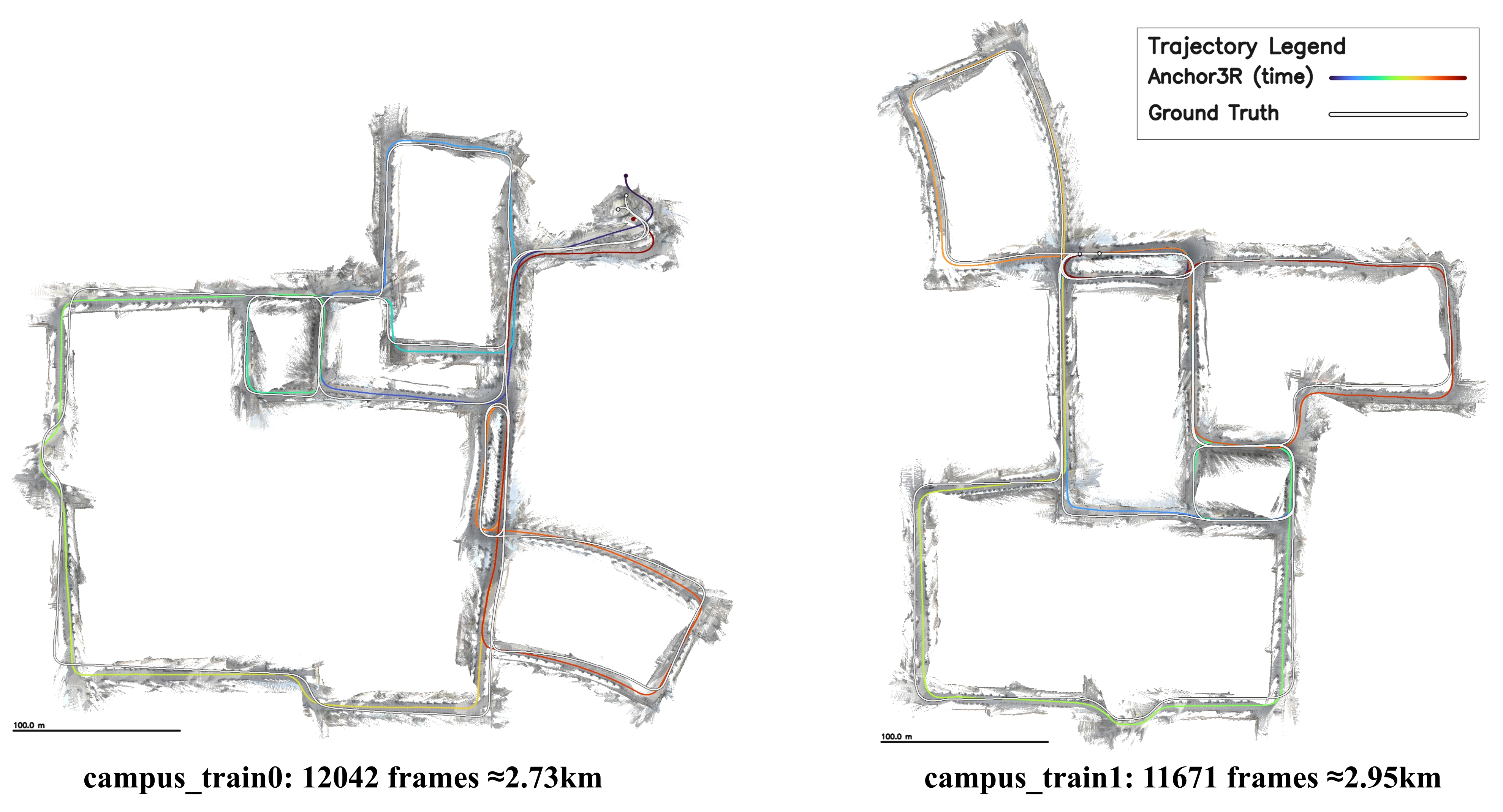
At a glance
Anchor3R predicts recent cameras relative to each incoming image, then combines these local measurements in a pose graph. Its transformer caches image evidence while rebuilding pose queries for every window. Online inference has bounded accelerator memory; optional offline loop retrieval and motion averaging further reduce drift. Experiments replay real datasets, with no physical-robot deployment and no constant bound on total map storage.
1 Introduction
Maintaining a distant coordinate origin inside a recurrent reconstruction model can couple local geometry with accumulated drift. Anchor3R instead uses each current image as a transient reference, leaving global alignment to an explicit graph. Overlapping windows contribute redundant relative-pose constraints, making later refinement possible.
The distinction matters operationally: strict online prediction has no loop detection and only estimates the new pose, whereas offline refinement revisits the graph and adds long-range constraints. The latter produces the strongest long-trajectory results.
2 Related Work
Classical SfM and SLAM.
Incremental structure from motion uses correspondence geometry, camera registration, triangulation and bundle adjustment. Global approaches and motion averaging separate relative measurements from global recovery. Anchor3R keeps this decomposition while learning the relative measurements.
Offline Feed-forward Reconstruction.
DUSt3R, VGGT and π³ provide feed-forward geometric priors. Chunked or stateful methods such as VGGT-Long, ZipMap and LoGeR extend scale, chiefly through offline/chunk processing. Anchor3R makes local measurements as frames arrive and exposes them for graph refinement.
Streaming Feed-forward Reconstruction.
CUT3R, STream3R, WinT3R and LongStream use persistent state, causal caches or compact camera pools. Anchor3R avoids carrying explicit historical pose-query states between local reference frames; its image cache and motion graph serve different purposes.
3 Method
A bounded window predicts relative poses plus a pointmap in the newest camera frame. Online medians combine those predictions with recovered historical poses. Offline robust rotation/position averaging uses the accumulated graph and optional loop edges to redistribute drift.
3.1 Current-Centric Formulation
The active window contains at most W recent frames. Equation 1 maps the current camera into each source camera; the current-to-current transform is identity. Each earlier frame supplies an edge to the current anchor. Overlap creates redundant short-range constraints, rather than only one consecutive-frame chain.
“Dense” describes this local measurement graph, not every pair in the entire recording. With fixed W, edge storage grows approximately linearly with sequence length. Local pointmaps are aligned by recovered global poses.
Equation 1
| (1) |
3.2 Sliding-Window Pose-Query Transformer
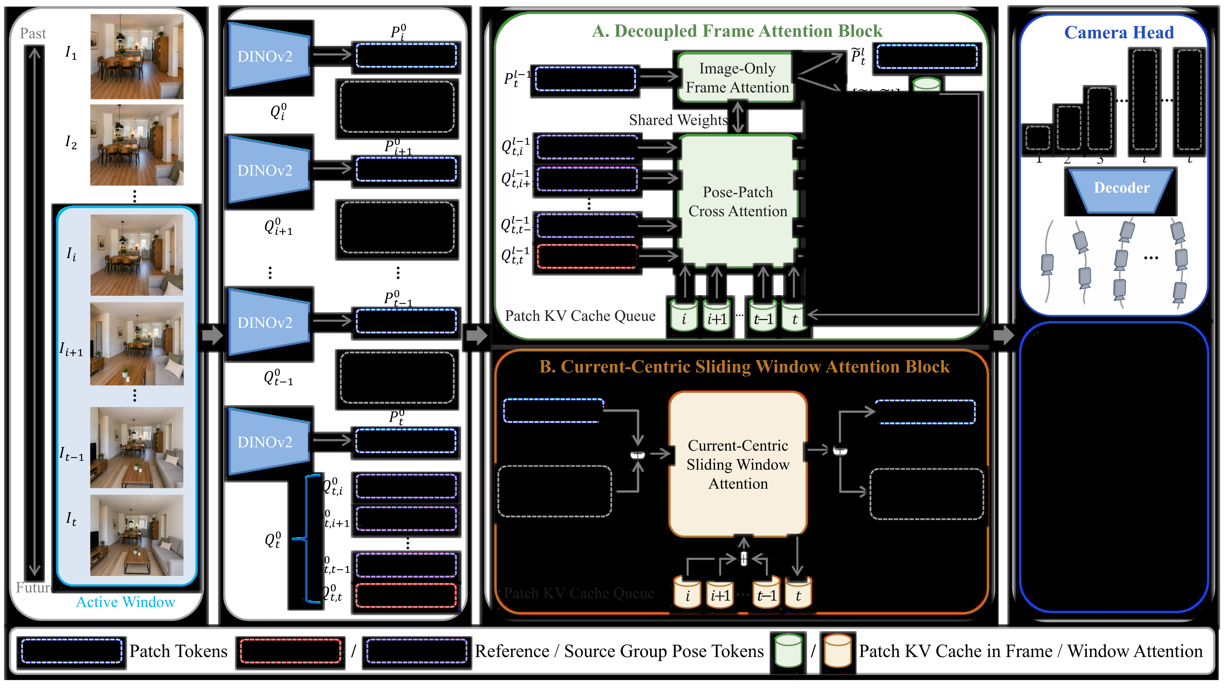
DINOv2 supplies patch features. Every active frame gets one pose token plus 31 registers, with different learned templates for current-reference and source frames. Decoupled frame attention computes image features; pose queries read their corresponding image states. Window attention combines the current patches and all active pose-query groups.
Only image-side keys/values are cached; pose-query states are discarded and recreated. This avoids explicitly reusing hypotheses tied to a previous reference. The equations below retain the grouping and attention operations; the empirical ablation supports this cache design without establishing a formal independence guarantee.
Equations
3.3 Prediction Heads
The camera head jointly decodes the first token of each query group because the outputs share one current-frame reference. A DPT-style head combines multiple patch-feature levels to output three local coordinates and one confidence value per pixel. Historical pointmaps are not re-predicted after later observations.
Equations
3.4 Motion Graph and Pose Recovery
World-to-camera rotations define relative rotation RᵢRₜᵀ. Rotating a predicted relative translation back by Rᵢᵀ gives a displacement from historical center cᵢ to cₜ. Online inference aggregates candidate current rotations through iterative Lie-algebra medians and candidate centers through coordinate-wise medians.
Offline refinement fixes a gauge, applies robust rotation averaging, then solves an L1 center problem with ADMM. Retrieved old views can be reinserted to predict loop edges. This can redistribute errors, but does not guarantee a globally accurate reconstruction or repair inconsistent learned scales.
Equation 2
| (2) |
3.5 Training
Training objectives.
The objective combines relative-camera supervision with confidence-weighted point reconstruction and spatial-gradient matching. A shared L1-fitted scale multiplies both predicted translations and pointmaps; a negative log-confidence term discourages trivially suppressing residuals. The exact four loss/scale expressions are retained below. This encourages consistency without establishing absolute metric scale.
Equations
Training data.
Training mixes sixteen real/synthetic sources: WildRGB, ScanNet, HyperSim, Mapillary, Replica, Mapfree, TartanAir, MVS-Synth, Virtual KITTI, Aria Synthetic Environments, Spring, Waymo, BlendedMVS, Co3Dv2, MegaDepth and DL3DV. Pose-guided sampling makes overlapping sequences from unordered data; random temporal spacing and block shuffling augment videos.
Implementation details.
VGGT initializes a 24-layer, approximately 1.2-billion-parameter model. Training unrolls 48 frames with W=10, one pose token plus 31 registers per frame, and images at most 518 pixels on their longer side. AdamW uses peak rate 10⁻⁴, cosine decay and 2,000 warm-up steps. Eighty thousand iterations on 32 A800 GPUs take about twelve days.
4 Experiments
Evaluation covers full replayed driving, indoor and mobile-mapping sequences. Main sequences are excluded from training; Waymo evaluation uses nine held-out segments from its official training split. Small-model diagnostic ablations use Virtual KITTI, which is also among training sources.
Original selectable table
| Methods | KITTI [15] (ATE ) | Avg. | ||||||||||
| 00 | 01 | 02 | 03 | 04 | 05 | 06 | 07 | 08 | 09 | 10 | ||
| 4541, 3.7 km | 1101, 2.5 km | 4661, 5.1 km | 801, 0.6 km | 271, 0.4 km | 2761, 2.2 km | 1101, 1.2 km | 1101, 0.7 km | 4071, 3.2 km | 1591, 1.7 km | 1201, 0.9 km | ||
| FastVGGT | * | 705.39 | * | 62.38 | 10.27 | 157.74 | 124.43 | 69.27 | * | 190.10 | 194.75 | 189.29 |
| MASt3R-SLAM | * | 530.37 | * | 18.87 | 88.98 | 159.430 | 92.00 | * | * | * | * | 177.93 |
| VGGT-SLAM | * | 607.16 | * | 169.83 | 13.12 | * | * | * | * | * | * | 263.37 |
| VGGT-Long | 8.64 | 21.20 | 52.72 | 8.78 | 4.20 | 9.88 | 4.67 | 2.66 | 72.98 | 31.84 | 27.71 | 25.94 |
| CUT3R | 185.89 | 651.52 | 296.98 | 148.06 | 22.17 | 155.61 | 132.54 | 77.03 | 238.39 | 205.94 | 193.39 | 209.78 |
| TTT3R | 190.93 | 546.84 | 218.77 | 105.28 | 11.62 | 153.12 | 132.94 | 70.95 | 180.57 | 211.01 | 133.00 | 177.73 |
| STream3R | 190.98 | 681.95 | 301.40 | 158.25 | 102.73 | 159.85 | 135.03 | 90.37 | 261.15 | 216.31 | 207.49 | 227.77 |
| StreamVGGT | 191.93 | 653.06 | 303.35 | 157.50 | 108.24 | 160.46 | 133.71 | 89.00 | 263.95 | 216.69 | 209.80 | 226.15 |
| LongStream | 92.55 | 46.01 | 134.70 | 3.81 | 1.95 | 84.69 | 23.12 | 14.93 | 62.07 | 85.61 | 21.48 | 51.90 |
| Anchor3R-Online | 44.18 | 48.43 | 149.61 | 4.39 | 1.99 | 62.63 | 12.12 | 10.39 | 52.12 | 55.23 | 8.57 | 40.89 |
| Anchor3R-Offline | 19.68 | 48.62 | 75.75 | 4.22 | 1.90 | 7.56 | 6.36 | 7.63 | 49.34 | 49.02 | 8.00 | 25.03 |
Original selectable table
| Method | VBR [5] ATE | Avg. | ||||||
| campus_train0 | campus_train1 | ciampino_train1 | colosseo_train0 | diag_train0 | pincio_train0 | spagna_train0 | ||
| 12042, 2.73 km | 11671, 2.95 km | 18846, 5.20 km | 8815, 1.45 km | 10021, 1.02 km | 11142, 1.27 km | 14141, 1.56 km | ||
| VGGT-SLAM | 93.51 | 71.74 | 124.10 | 101.00 | 33.64 | 66.42 | 57.00 | 78.20 |
| VGGT-Long | 118.59 | 98.21 | 172.13 | 39.56 | 30.80 | 53.44 | 50.27 | 80.43 |
| Pi3-Chunk | 78.50 | 65.77 | 111.72 | 77.09 | 23.81 | 41.99 | 44.76 | 63.38 |
| InfiniteVGGT | 123.65 | 100.00 | * | 83.91 | 31.58 | 70.73 | 56.25 | 91.60 |
| LongStream | 100.57 | 105.55 | 131.78 | 72.52 | 32.35 | 43.47 | 59.31 | 77.93 |
| Anchor3R-Online | 86.63 | 82.16 | 168.25 | 61.43 | 29.38 | 51.34 | 54.34 | 76.21 |
| Anchor3R-Offline | 5.13 | 3.52 | 78.64 | 17.25 | 5.35 | 15.56 | 11.76 | 19.60 |
4.1 Camera Pose Estimation
Evaluation protocol.
Trajectories receive a similarity alignment before absolute trajectory error is measured. This removes global scale as well as rigid gauge error; it does not assess absolute metric-scale accuracy. Failed runs are excluded from averages, so methods with failures are not averaged over the same successful-sequence set.
Online mode processes frames once in temporal order, without loop retrieval. Offline mode selects every fifth frame as a keyframe, retrieves three similar views with NetVLAD, reinserts temporally separated matches and averages the augmented motion graph.
Results.
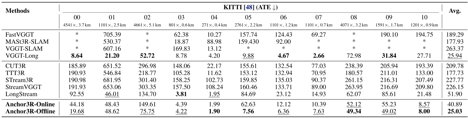
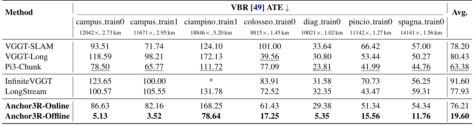
On KITTI, average aligned error falls from LongStream 51.90 m to Anchor3R-Online 40.89 m and Offline 25.03 m. Offline wins the main-table average, not every route. On VBR, Online 76.21 m only slightly improves over LongStream 77.93 m; Offline 19.60 m is best across the main table’s seven routes.
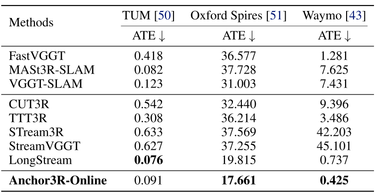
Table 3 reports Online 0.091 m on TUM, 17.661 m on Oxford Spires and 0.425 m on Waymo. Oxford/Waymo are best in that table; TUM trails LongStream 0.076 and MASt3R-SLAM 0.082. Appendix D’s matched-backend comparison further qualifies the offline ranking.
Original selectable table
| Methods | TUM [41] | Oxford Spires [43] | Waymo [42] |
| ATE | ATE | ATE | |
| FastVGGT | 0.418 | 36.577 | 1.281 |
| MASt3R-SLAM | 0.082 | 37.728 | 7.625 |
| VGGT-SLAM | 0.123 | 31.003 | 7.431 |
| CUT3R | 0.542 | 32.440 | 9.396 |
| TTT3R | 0.308 | 36.214 | 3.486 |
| STream3R | 0.633 | 37.569 | 42.203 |
| StreamVGGT | 0.627 | 37.255 | 45.101 |
| LongStream | 0.076 | 19.815 | 0.737 |
| Anchor3R-Online | 0.091 | 17.661 | 0.425 |
Original selectable table
| Methods | 7Scenes | TUM | ||
| CD | F1@0.25 | CD | F1@0.25 | |
| FastVGGT | 6.373 | 0.710 | 0.104 | 0.926 |
| MASt3R-SLAM | 5.987 | 0.691 | 0.057 | 0.954 |
| VGGT-SLAM | 6.306 | 0.696 | 1.993 | 0.633 |
| CUT3R | 6.281 | 0.274 | 0.474 | 0.533 |
| TTT3R | 6.231 | 0.260 | 0.249 | 0.792 |
| STream3R | 6.353 | 0.479 | 1.126 | 0.444 |
| StreamVGGT | 6.630 | 0.483 | 0.680 | 0.402 |
| LongStream | 2.260 | 0.641 | 0.225 | 0.673 |
| Anchor3R-Online | 1.848 | 0.707 | 0.108 | 0.933 |
4.2 3D Reconstruction
Evaluation protocol.
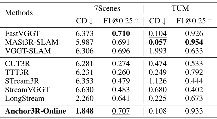
Predicted poses and pointmaps form a cloud, which is similarity-aligned to ground truth. Evaluation uses Chamfer distance and F1 at threshold 0.25 on 7Scenes and TUM. These aligned geometry metrics do not validate unaligned global scale.
Results.
On 7Scenes, Online achieves Chamfer 1.848 and F1=0.707: best distance, but slightly below FastVGGT’s F1=0.710. On TUM, 0.108/0.933 trails MASt3R-SLAM 0.057/0.954; FastVGGT also has slightly smaller distance 0.104. The method improves streaming map consistency without universally beating optimization-based systems.
4.3 Ablation and Analysis
Most diagnostics use a ViT-Small model on Virtual KITTI. They test design choices but are not identical in scale or distribution to the main 1.2B model.
Current-centric prediction.
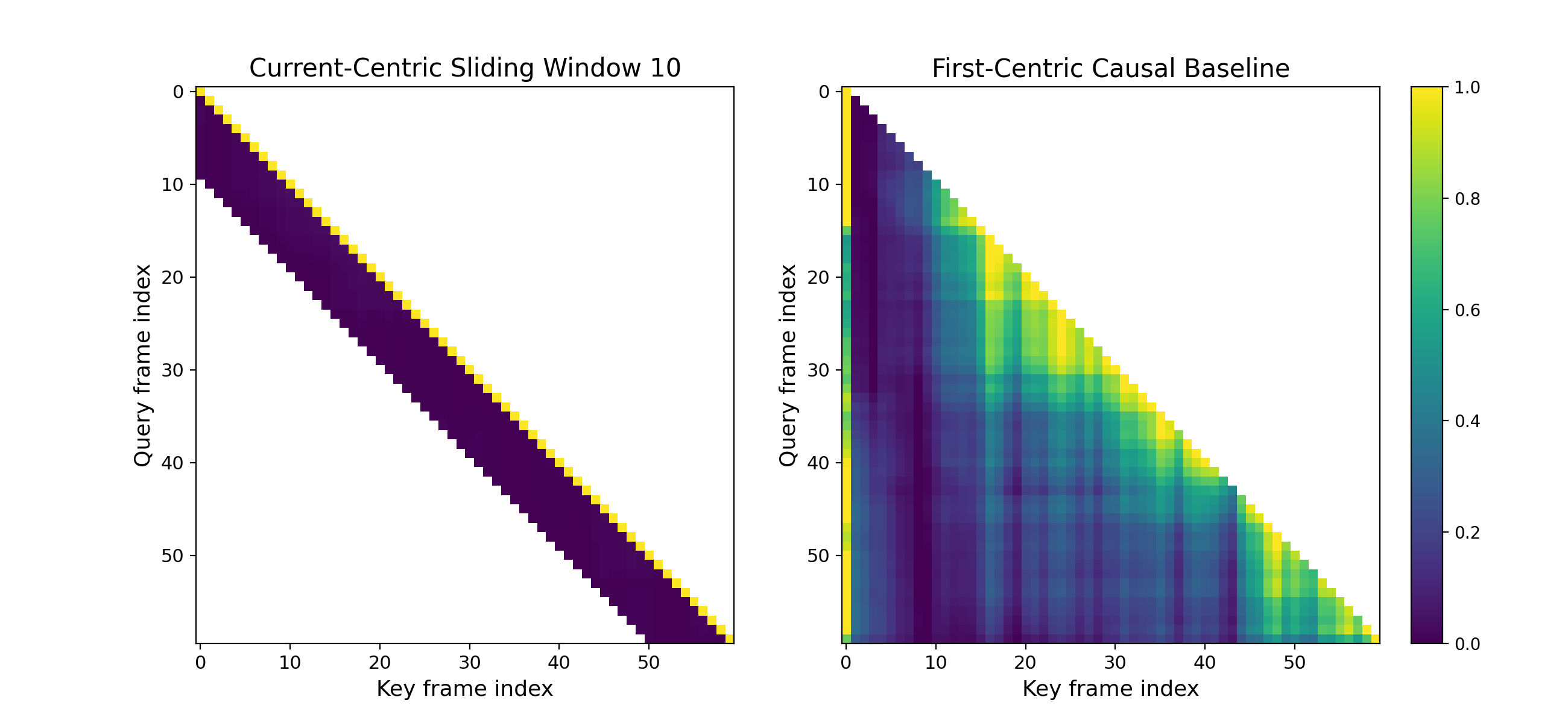
Sixty-frame attention maps contrast persistent first-frame attention with support moving along the current window. This illustrates the intended local-reference behavior; attention visualization alone does not establish the cause of all accuracy gains.
Image-only key/value cache.
Removing cached pose tokens lowers mean ATE 3.517→2.642, relative translation error 0.146→0.097 and relative rotation error 0.092→0.090. Most cells improve, with exceptions visible in Table 5. Reinstantiating queries helps empirically; image features still participate in window attention.

Original selectable table
| Methods | Scene 01 | Scene 02 | Scene 06 | Scene 18 | Scene 20 | Avg. | ||||||||||||
| ATE | RTE | RRE | ATE | RTE | RRE | ATE | RTE | RRE | ATE | RTE | RRE | ATE | RTE | RRE | ATE | RTE | RRE | |
| w pose cache | 3.613 | 0.177 | 0.132 | 2.174 | 0.111 | 0.074 | 0.285 | 0.037 | 0.055 | 3.955 | 0.195 | 0.087 | 7.558 | 0.211 | 0.112 | 3.517 | 0.146 | 0.092 |
| w/o pose cache | 3.113 | 0.101 | 0.127 | 1.054 | 0.084 | 0.073 | 0.424 | 0.042 | 0.059 | 1.410 | 0.118 | 0.080 | 7.208 | 0.142 | 0.110 | 2.642 | 0.097 | 0.090 |
Active window size.
Increasing the small-model window 5→10 improves ATE 3.23→2.64, rotation 0.12→0.09 and translation 0.15→0.10. Window 15 gives 2.55/0.08/0.10 but reduces speed 27.5→22.9 FPS and raises reported iteration time 2.7→3.2 s. W=10 is the selected trade-off.
Runtime and memory scaling.
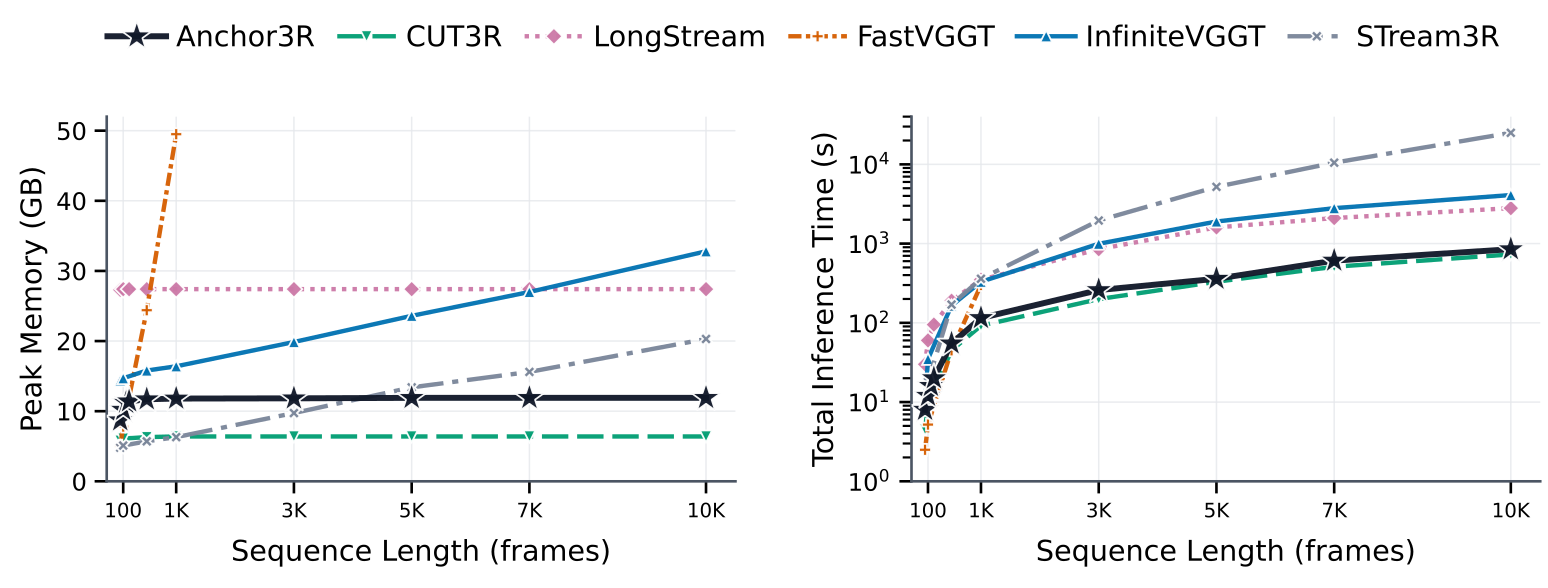
The full model runs at 12.7 FPS with 11.9 GB peak accelerator memory; measured inference time grows approximately linearly through 10,000 frames. Memory boundedness applies to online accelerator state. Graphs and pointmaps on processor memory/disk grow with the recording, and offline global solving is an additional stage.
Reported motion-averaging times are 11.88 s for 12K and 17.24 s for 18.8K frames. These are solver timings, not an end-to-end bound for retrieval, anchor reinsertion, prediction and refinement. Training uses 48-frame clips; long-sequence inference is tested, not guaranteed for arbitrary duration.
Controlled offline refinement.
Applying the same retrieval/refinement protocol helps other models too. Anchor3R wins all seven routes against LongStream-Off-5 and six against VGGT-Off-5. However, VGGT-Off-5 has the better average: 16.96 m versus 19.60 m, because its ciampino error 28.30 m is much below Anchor3R’s 78.64 m. Route-win count and aggregate error tell different stories.
5 Limitations
Pointmaps are predicted once, so pose refinement cannot update their local geometry. Relative-scale inconsistency can degrade averaging. Highly dynamic scenes lack dedicated evaluation, loop retrieval/alignment remain separate from the learned model, and all experiments are dataset replay without physical-robot deployment.
6 Conclusion
Current-frame-relative prediction, transient pose queries and graph recovery make long streams practical and correctable. The evidence supports bounded online accelerator memory and improved aligned trajectories/maps, with substantial gains from offline loop constraints and remaining scale, dynamics and difficult-turn failures.
Acknowledgments
Support is acknowledged from the National Natural Science Foundation of China and Beijing Natural Science Foundation.
Supplementary Material
Appendix A Online Motion Averaging
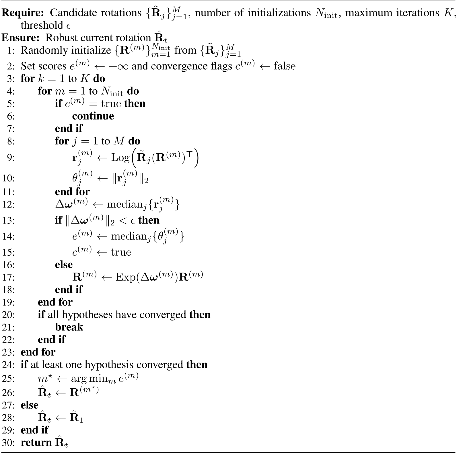
Each historical pose and relative rotation induces a candidate current rotation. Algorithm 1 runs several randomly initialized hypotheses, computes coordinate-wise medians of logarithmic rotation residuals, and left-multiplies the corresponding exponential update. It selects the converged hypothesis with smallest median angular residual; if none converges, it returns the first candidate.
Candidate camera centers are aggregated by coordinate-wise median without iteration. Small-angle handling and multiple initializations improve numerical robustness, but the median procedure has no stated global-optimality guarantee. Previously recovered poses remain fixed in this online update.
Equations 3–8
| (3) |
| (4) |
| (5) |
| (6) |
| (7) |
| (8) |
Original selectable algorithm
Appendix B Offline Motion Averaging
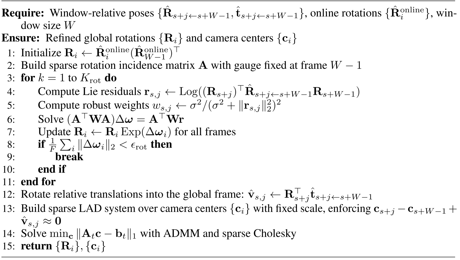
Offline recovery jointly uses local-window edges and any reinserted loop edges. Online estimates initialize the rotations; one reference frame fixes the gauge. This global pass is distinct from the causal online update.
Rotation averaging.
Equations 9–14 and Algorithm 2 retain the exact rotation procedure. Right-trivialized residuals are linearized into a sparse incidence system; Geman–McClure-style weights use a five-degree scale. Weighted normal equations produce axis-angle increments, applied by right multiplication until the mean increment is small or the iteration limit is reached.
These are robust local iterative updates, not a proof that all corrupted loop or local measurements will be rejected. The arbitrary reference gauge is removed again by evaluation alignment.
Equations 9–14
| (9) |
| (10) |
| (11) |
| (12) |
| (13) |
| (14) |
Position averaging.
After rotations are fixed, relative translations are rotated into the global frame. Equations 15–17 solve least absolute deviations in camera centers with one center fixed. ADMM uses a sparse Cholesky-accelerated update.
There are no independent per-window scale variables. This preserves learned translation/pointmap scale relationships but also means inconsistent scales cannot be freely absorbed by the optimizer. The recovered poses transform the already predicted local pointmaps.
Equations 15–17
| (15) |
| (16) |
| (17) |
Original selectable algorithm
Appendix C Additional Ablation on Online and Offline Motion Averaging
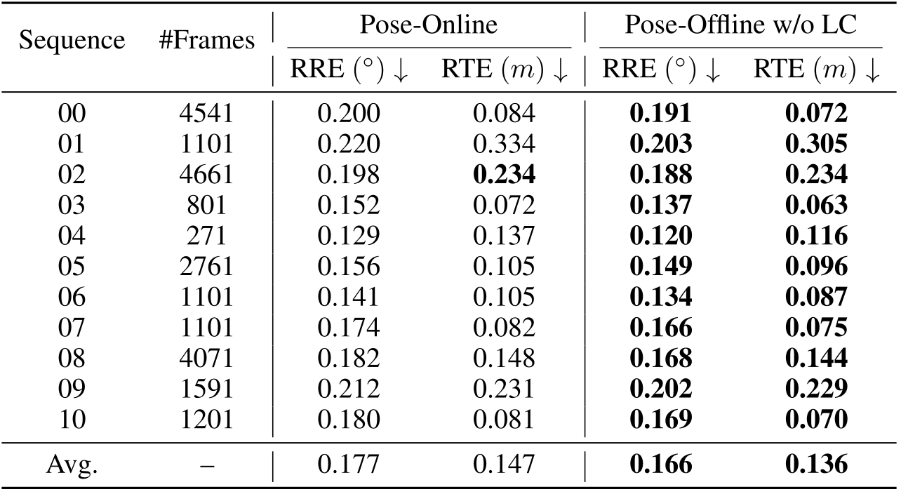
Without any loop edges, offline averaging improves mean KITTI relative rotation error 0.177°→0.166° and translation error 0.147 m→0.136 m. Sequence 02 translation remains 0.234 m at the reported precision. Local redundancy helps, while these metrics do not establish elimination of global drift.
Original selectable table
| Sequence | #Frames | Pose-Online | Pose-Offline w/o LC | ||
| RRE | RTE | RRE | RTE | ||
| 00 | 4541 | 0.200 | 0.084 | 0.191 | 0.072 |
| 01 | 1101 | 0.220 | 0.334 | 0.203 | 0.305 |
| 02 | 4661 | 0.198 | 0.234 | 0.188 | 0.234 |
| 03 | 801 | 0.152 | 0.072 | 0.137 | 0.063 |
| 04 | 271 | 0.129 | 0.137 | 0.120 | 0.116 |
| 05 | 2761 | 0.156 | 0.105 | 0.149 | 0.096 |
| 06 | 1101 | 0.141 | 0.105 | 0.134 | 0.087 |
| 07 | 1101 | 0.174 | 0.082 | 0.166 | 0.075 |
| 08 | 4071 | 0.182 | 0.148 | 0.168 | 0.144 |
| 09 | 1591 | 0.212 | 0.231 | 0.202 | 0.229 |
| 10 | 1201 | 0.180 | 0.081 | 0.169 | 0.070 |
| Avg. | – | 0.177 | 0.147 | 0.166 | 0.136 |
Appendix D Controlled Offline Refinement on VBR
Matched refinement improves LongStream on six of seven routes and VGGT on all seven. Anchor3R’s 6/7 wins over VGGT-Off-5 coexist with a worse mean 19.60 versus 16.96. Its difficult ciampino route dominates this difference.
Keyframe spacing 5/10/15 gives mean 19.60/21.80/23.89 m. Most routes stay broadly similar, but ciampino degrades 78.64→92.51→100.87 m. Sparse retrieval is therefore not uniformly harmless.

Original selectable table
| Method | campus_train0 | campus_train1 | ciampino_train1 | colosseo_train0 | diag_train0 | pincio_train0 | spagna_train0 | Avg. |
| LongStream | 100.57 | 105.55 | 131.78 | 72.52 | 32.35 | 43.47 | 59.31 | 77.93 |
| LongStream-Off-5 | 87.61 | 99.86 | 98.64 | 45.99 | 8.46 | 65.84 | 39.77 | 63.74 |
| VGGT-Long | 118.59 | 98.21 | 172.13 | 39.56 | 30.80 | 53.44 | 50.27 | 80.43 |
| VGGT-Off-5 | 12.20 | 9.85 | 28.30 | 20.21 | 12.84 | 19.77 | 15.56 | 16.96 |
| Anchor3R-Off-5 | 5.13 | 3.52 | 78.64 | 17.25 | 5.35 | 15.56 | 11.76 | 19.60 |
| Anchor3R-Off-10 | 5.02 | 2.91 | 92.51 | 19.15 | 5.21 | 16.51 | 11.27 | 21.80 |
| Anchor3R-Off-15 | 5.15 | 3.62 | 100.87 | 21.65 | 5.04 | 18.77 | 12.11 | 23.89 |
Appendix E Failure Case Analysis
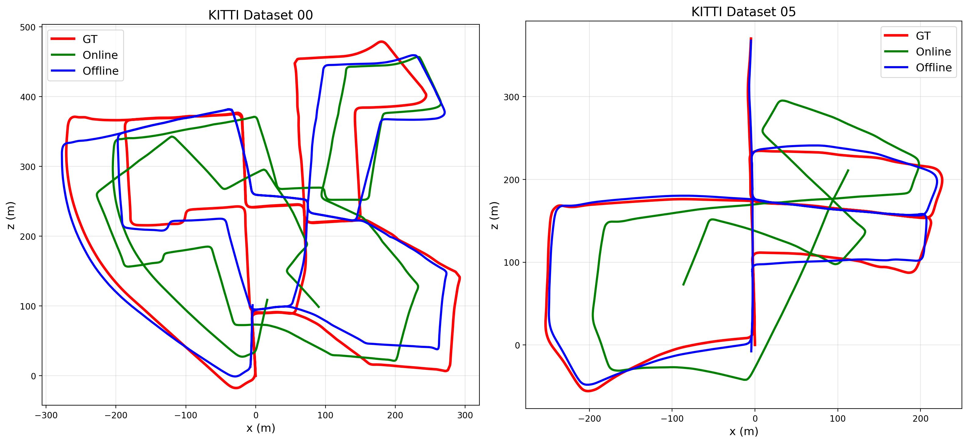
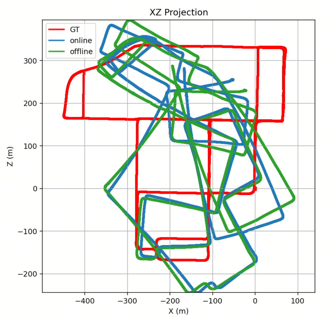
Figure 6 shows ciampino trajectories without loop constraints. Frequent turns produce orientation errors that redirect subsequent translations; local averaging alone leaves substantial drift. The figure does not show the fully loop-refined result, whose remaining error is separately reported in Table 7.
Appendix F Evaluation Dataset Details
Evaluation uses complete sequences without frame subsampling: all seven VBR routes, 8,815–18,846 frames and up to 5.2 km; all eleven KITTI camera 02 streams; all twelve Oxford front-camera subsets; sequence 01 of each of the seven 7Scenes scenes; and full TUM sequences.
Waymo uses nine held-out segments, 196–199 frames and 42–351 m each: 163453191, 183829460, 315615587, 346181117, 371159869, 405841035, 460417311, 520018670 and 610454533. The dataset participates in training, but these segments do not.