Overview
OSCAR learns how long observed obstacle classes tend to block known routes, then chooses a waiting deadline before rerouting.
At a glance
A route-following robot should sometimes wait for a short-lived obstacle and sometimes take a detour around a persistent one. OSCAR learns class-specific residual clearance-time distributions, including observations censored when the robot leaves before clearance. A time-dependent graph planner combines these distributions with remembered blockages to choose patience thresholds. Simulated mean travel time approaches a distribution-aware oracle, and physical atrium experiments show adaptation over fifty staged episodes. The method assumes a route graph and usable obstacle labels; it complements local avoidance rather than replacing it.
1 Introduction
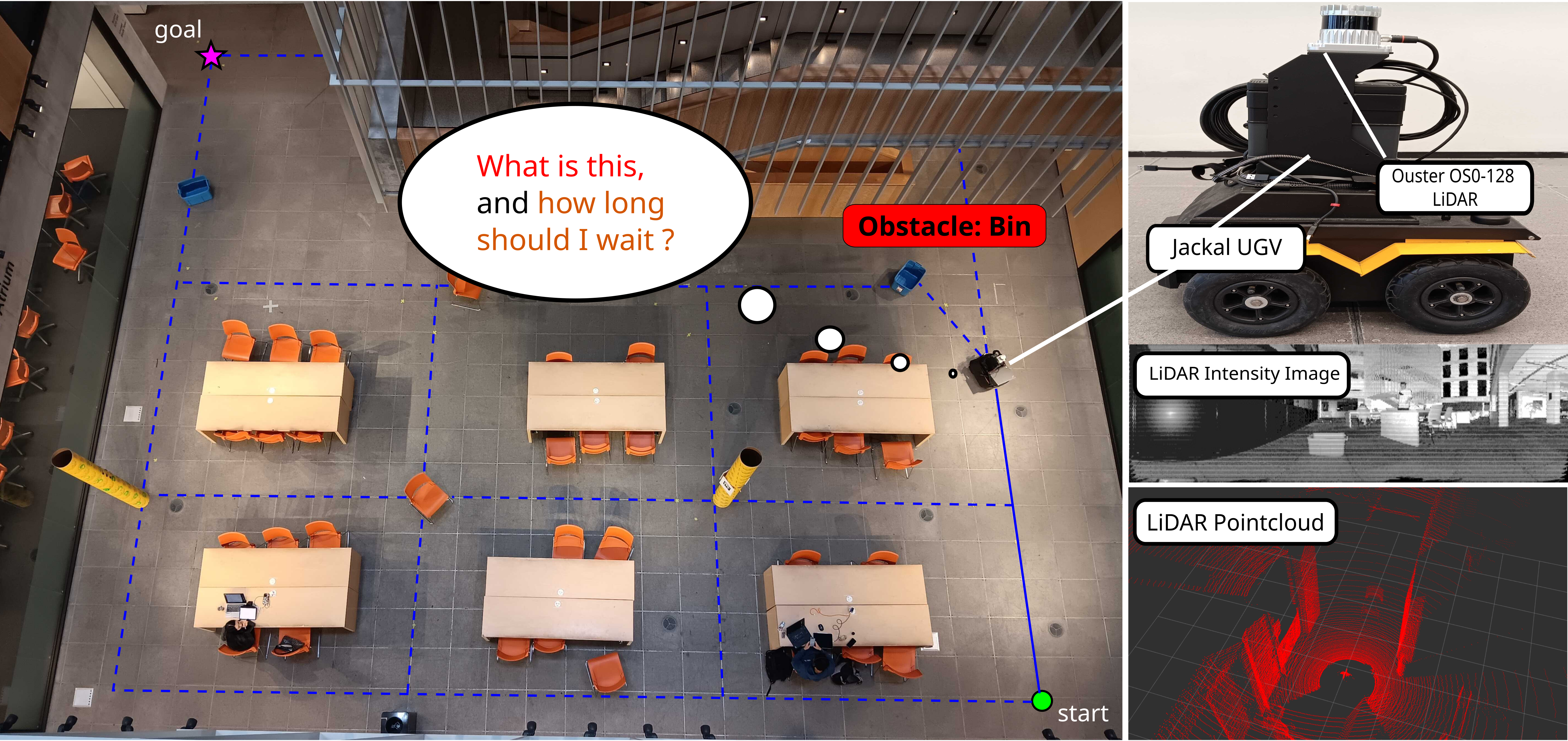
The decision applies when an edge cannot be safely bypassed locally, such as a narrow corridor or designated route. A person and a parked object may warrant different waiting policies, but fixed class rules cannot adapt to actual persistence. OSCAR learns clearance statistics from repeated encounters and incorporates remembered obstacles elsewhere on the graph. Its objective is expected time-to-goal under a navigation-cost model, not a global safety or socially optimal behavior guarantee.
2 Related Work
Local obstacle avoidance chooses short-horizon motion, while this work chooses whether to persist with a blocked graph edge. The Canadian Traveller Problem supplies related online route uncertainty, but often treats blocked edges as static. Time-dependent routing supplies the FIFO condition needed for efficient shortest-path search. Kaplan–Meier estimation [17] supplies a nonparametric way to retain partial clearance observations rather than discarding long-lived obstacles when the robot reroutes.
3 OSCAR: Survival-Guided Wait-or-Reroute Planning
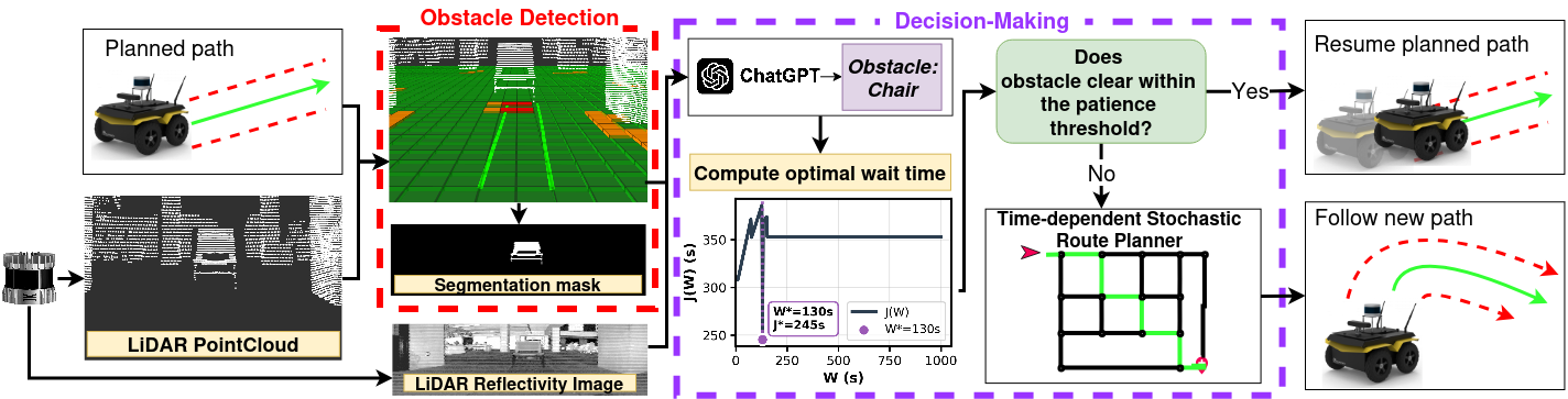
The graph has deterministic nominal edge traversal times, with temporary blockages encountered during travel. The robot observes an obstacle class, selects a maximum wait, and either continues after clearance or replans with that edge excluded. It learns over repeated episodes. The oracle knows the true distributions and class/blockage probabilities; it does not know the actual future clearance time of every obstacle.
3.1 Learning Class-Conditioned Obstacle Persistence
For each class, estimate the survival function of remaining blockage time measured from first encounter, not from obstacle creation. Each observed clearance multiplies the survival estimate by the fraction of at-risk observations that remain blocked. A reroute contributes a right-censored sample: the obstacle lasted at least that long, without falsely recording clearance. Independent censoring conditional on modeled variables is a required statistical assumption, as discussed in survival-analysis theory [18].
Equation 1
| (1) |
3.2 Arrival-Time-Dependent Edge Costs
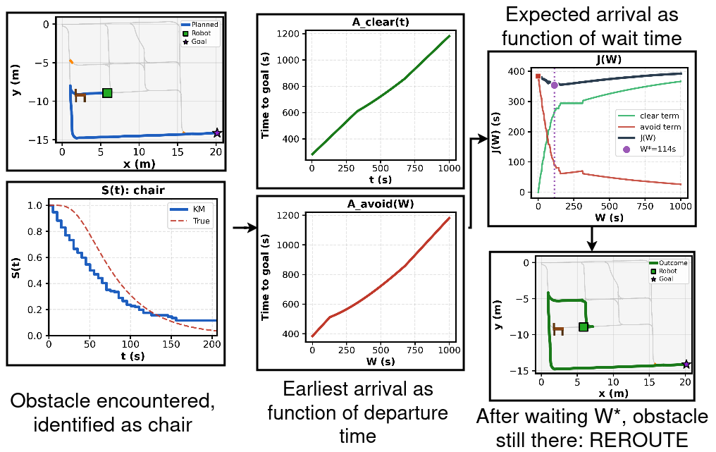
For an unremembered edge, expected delay combines the learned blockage rate, encountered-class frequencies, and class mean residual lifetimes. For a remembered edge, store class and first/last observation times. At a planned future arrival, condition survival on the last confirmed observation, then mix the expected remaining delay if the old obstacle persists with the ordinary new-blockage delay if it has cleared. These are shared class/graph estimates rather than edge-specific contextual models. Finite mean delays and defined survival-ratio denominators are necessary; handling an unobserved or incompletely observed survival tail is not fully specified.
3.3 Wait-or-Reroute Decision at a Blocked Edge
For each possible waiting threshold, average the time-to-goal over clearance before the threshold, then add the cost of waiting to the deadline and rerouting when the obstacle remains. Both terms include elapsed waiting from the original encounter, avoiding double counting. Minimize this expectation within a bounded horizon. With a Kaplan–Meier curve, clearance contributions become a finite sum over observed events.
Equations 2–3
| (2) |
| (3) |
3.3.1 Computing A clear and A avoid
After clearance, shortest-path planning may use the newly available edge but need not do so. After abandoning the wait, planning excludes that edge. Other remembered blockages make downstream costs depend on arrival time. The main method evaluates survival event times and horizon endpoints using time-dependent Dijkstra; the appendix develops the functional Bellman–Ford view. A separate implementation paragraph specifies 300-point grids, so the exact reported search discretization is not entirely consistent across descriptions.
3.4 Online Adaptation
Record the duration observed and whether clearance occurred, then update class statistics along with blocked-edge and class frequencies. The main text describes an update after each encounter; the detailed simulation protocol instead freezes the model during an episode and updates from all accumulated observations afterward. Repeated visits can count as separate encounters because persistent physical obstacles are not explicitly associated across observations.
4 Experimental Evaluation of Survival-Guided Navigation
Simulation controls obstacle generation and provides an oracle comparison. Physical experiments validate integration with a taught route graph and semantic labeling, including a separate less-controlled person/chair setting.
4.1 Simulation Experiments
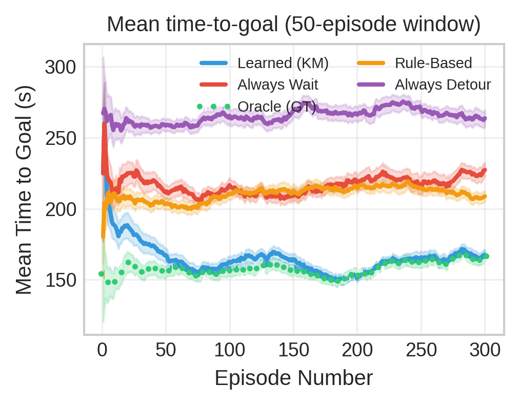
Over one thousand episodes per run and one hundred random seeds, OSCAR averages 160.7 seconds to goal versus 159.3 for the oracle, 185.9 without obstacle memory, 210.5 for a fixed class rule, 218.2 for always waiting, and 264.7 for always rerouting. All of these reach 100% success under the one-hour timeout. Greedy CTP reaches only 13.1% because it permanently forbids encountered blocked edges within each episode; timeout assignment drives its 3,135.7-second mean.
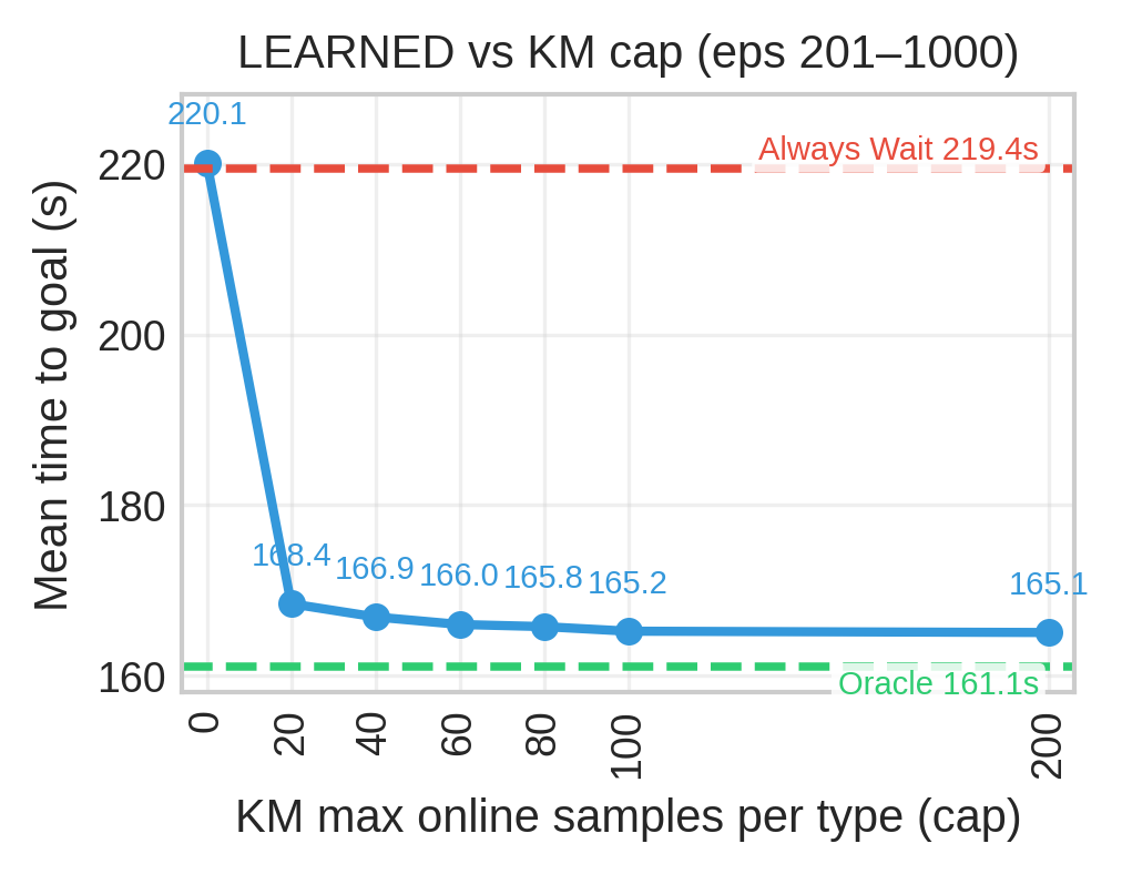
The learned policy is about 0.9% slower than this oracle on the reported mean. Sample-cap experiments indicate rapid gains with fewer than twenty observations per class, but do not provide a general sample-complexity guarantee. In a separate bimodal-lifetime ablation, retaining censored observations estimates residual clearance at 241.4 seconds versus a true 246.1, while discarding them yields 205.8.
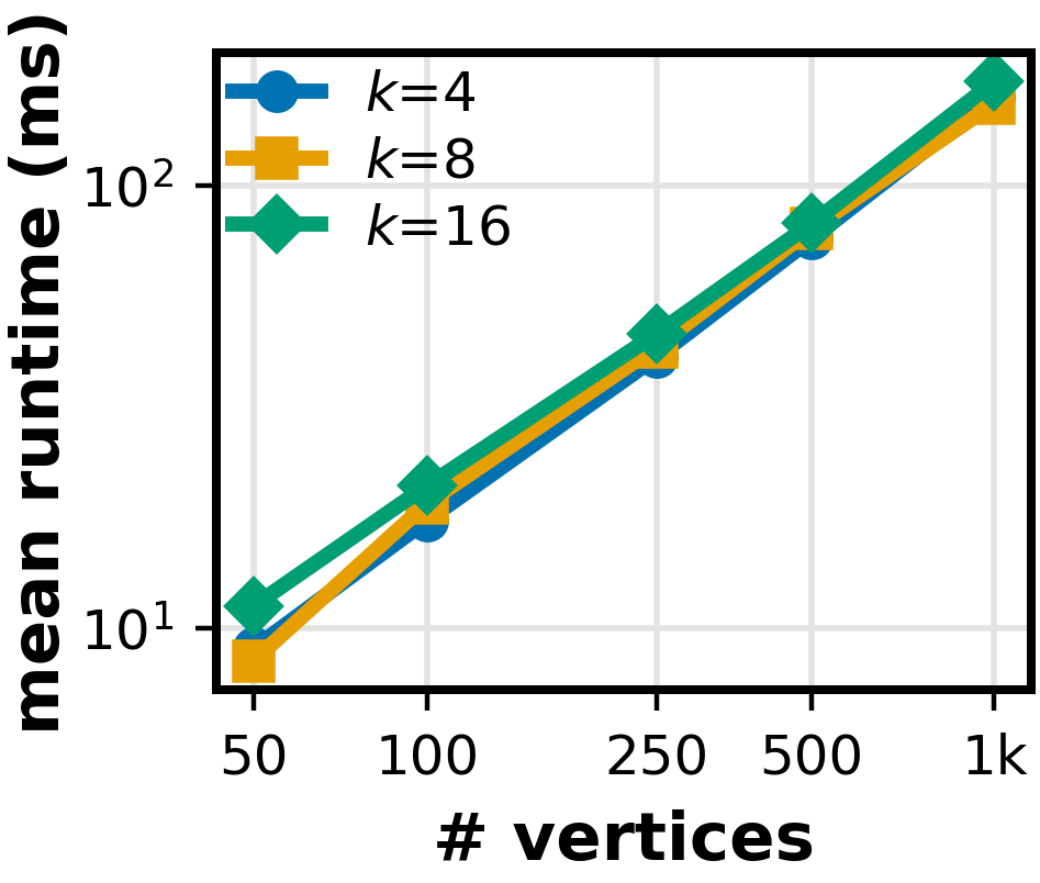
Planning benchmarks use 49–1,024 vertices and four, eight, or sixteen classes. At the largest tested graph, reported mean and 95th-percentile threshold-computation times are below 0.172 and 0.276 seconds. Candidate-time capping limits growth with accumulated data; this measured timing is not a guarantee for arbitrary graph density or history.

| Method | Time-to-goal (s) | Success rate | Reroutes | Waiting time | Blocked edges |
|---|---|---|---|---|---|
| Always Wait | 218.2 | 100.0% | 0.0 | 186.2 | 2.8 |
| Always Reroute | 264.7 | 100.0% | 24.2 | 0.0 | 24.2 |
| Rule-Based | 210.5 | 100.0% | 11.9 | 29.0 | 16.1 |
| Greedy CTP | 3135.7 | 13.1% | 3.4 | 0.0 | 2.5 |
| OSCAR w/o Memory | 185.9 | 100.0% | 1.8 | 149.8 | 4.5 |
| OSCAR (Ours) | 160.7 | 100.0% | 0.5 | 121.9 | 3.4 |
| Oracle | 159.3 | 100.0% | 0.5 | 121.7 | 3.3 |
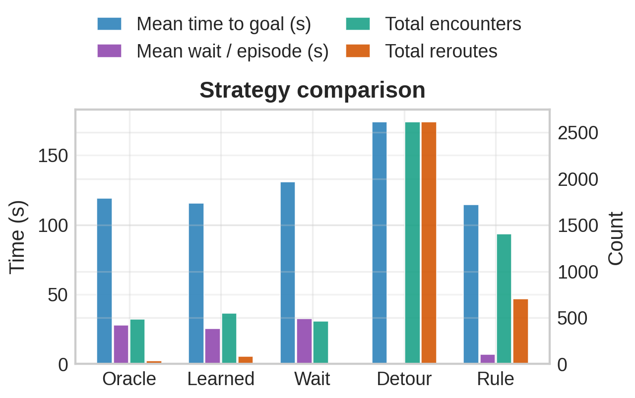
(a) Strategy comparison
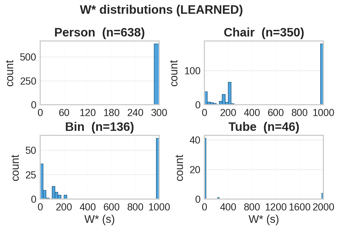
(b) Learned patience thresholds
4.2 Real-World Experiments
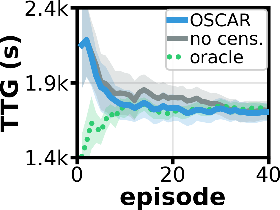
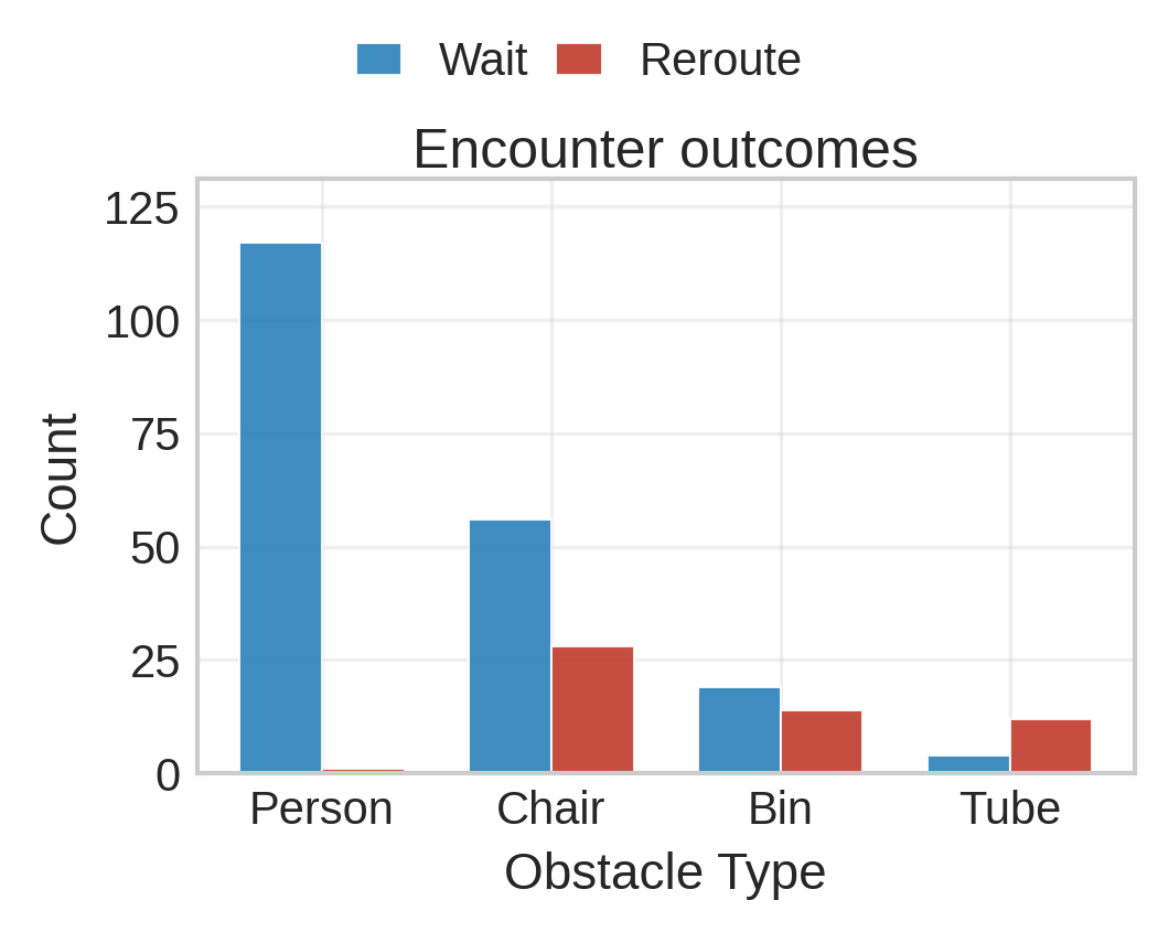
A physical robot follows an atrium route network using teach-and-repeat navigation [9]. A vision–language model labels masked lidar reflectivity images as person, chair, bin, or tube; the graph planner then chooses the wait. Fifty main episodes recreate simulator-generated placement and clearance schedules. Travel time improves toward roughly two hundred seconds and compares favorably with always waiting in the plotted deployment.
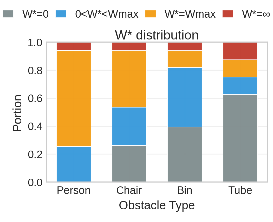
People usually receive long waits, chairs and bins mixed waiting/rerouting, and tubes frequent immediate reroutes. Maximum waits are chosen empirically from objective curves. Infinite-wait cases mean no alternate path exists, rather than an inferred finite clearance deadline. These staged physical results establish integration and adaptation under controlled scenarios, not an unbiased evaluation of natural obstacle lifetimes.
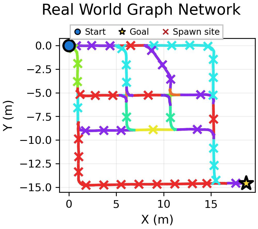
(a) Atrium graph
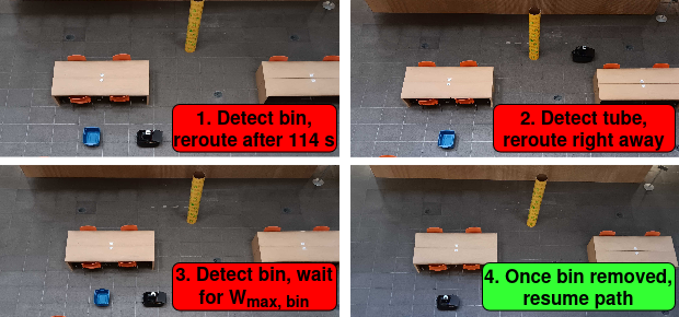
(b) Example obstacle encounter sequence
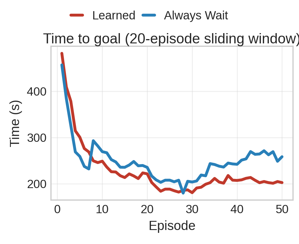
(a) Time-to-goal
(b) Wait vs. reroute decisions
(c) Selected patience thresholds
5 Limitations and Future Work
The reroute estimate treats the alternative as a committed route and does not fully account for later replanning, potentially making detours look too expensive. Kaplan–Meier estimation also relies on noninformative censoring. Adaptive deadlines do not automatically violate that assumption in the class-conditioned simulator, but real context could affect both clearance time and the attractiveness of rerouting.
Spatially shared blockage statistics ignore route-specific activity; repeated encounters may concern the same physical obstacle; and labeling errors can choose the wrong survival model. More detailed contextual classes, obstacle association, and semantic priors are proposed improvements. The framework does not establish theoretical learning guarantees under all these feedback effects.
6 Conclusion
Survival learning, remembered blockages, and arrival-time-aware route costs provide an effective wait-or-reroute policy in the tested settings. Censored observations and memory both contribute. The result is near-oracle performance for the specified model and experiments, with broader real-world reliability depending on perception, context, and model assumptions.
Appendix Appendix A Functional Time-Dependent Planner and Proofs
The proof appendix establishes FIFO edge-arrival functions, monotone functional shortest-path costs, and a finite threshold candidate set for the Kaplan–Meier objective.
Appendix A.1 FIFO Edge Arrival Functions
For an unremembered edge, arrival time equals departure plus a constant expected cost, so it is monotone. For a remembered obstacle, multiply survival probability by conditional residual life to obtain an integrated survival tail divided by survival at last observation. Differentiating leaves nonnegative terms because survival cannot increase and elapsed age cannot decrease. For stepwise Kaplan–Meier curves, slopes are nonnegative between events and jumps cannot go downward. Thus the specified expected-cost model is FIFO, assuming valid denominators and finite integrals; this is a property of the planning approximation, not every possible stochastic traffic process.
Equations
Appendix A.2 Functional Bellman–Ford Computation
Functional Bellman–Ford propagates earliest-arrival functions rather than scalar times. Each relaxation composes the upstream function with the FIFO edge-arrival function and takes a pointwise minimum. Composition and minimum preserve monotonicity. Under Kaplan–Meier costs the functions are piecewise affine, with breakpoints introduced by survival events and route comparisons. The learned implementation evaluates candidate times with Dijkstra instead of explicitly propagating every function.
Equation
Clear case.
For the clearance case, initialize the current vertex’s arrival time to the clearance parameter and all other vertices to infinity. Mark the encountered edge available and relax graph edges for at most the number of vertices minus one passes. The resulting goal-arrival function includes both waiting and subsequent travel.
Equations
Avoid case.
For the avoidance case, initialize the current vertex at the patience deadline, remove the still-blocked edge, and perform the same functional relaxations. The goal-arrival function includes the abandoned wait and the best remaining route under the modeled downstream costs.
Equations
Appendix A.3 Monotonicity of A clear and A avoid
Both cases start from nondecreasing functions and preserve that property through every relaxation. Therefore delaying clearance or delaying abandonment cannot reduce total arrival time measured from the original encounter. Downstream expected waiting can decrease with later arrival, but the FIFO proof bounds that decrease so it cannot outweigh the extra elapsed wait.
Equations
Appendix A.4 Finite Candidate Set for the KM Objective
Between observed clearance events, no new probability mass enters the clearance sum and the survival weight stays constant. The only changing term is the nondecreasing avoid-route cost, so an interval’s best threshold lies at its left endpoint. Consequently zero and survival event times within the horizon suffice; adding the upper endpoint is harmless. This exact argument applies to the discrete estimated distribution, not an arbitrary continuous distribution or an approximate capped grid.
Equations
Appendix Appendix B Simulation Details
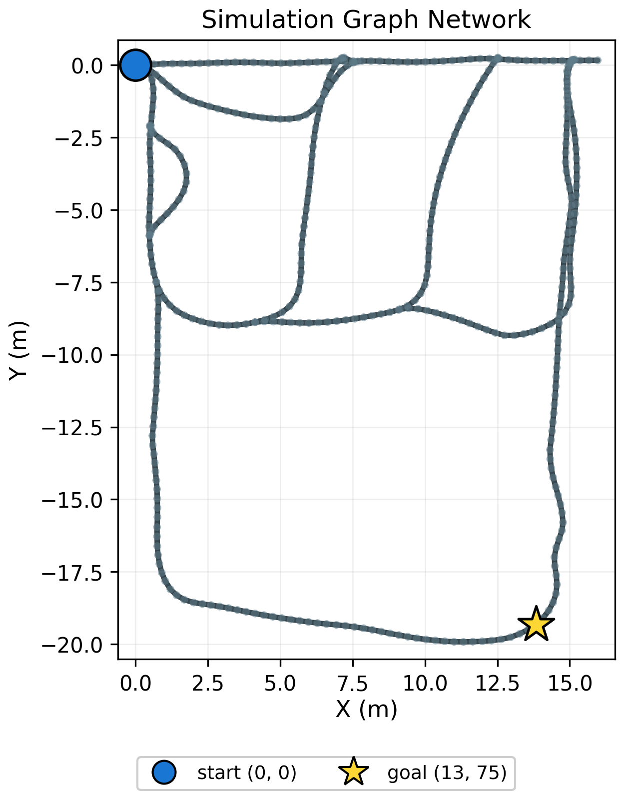
Simulation uses a known route network, fixed start, farthest goal vertex, and speed of 0.95 meters per second. Multiple routes permit nontrivial choices between waiting and detouring.
Appendix B.1 Ground-Truth Obstacle Distributions
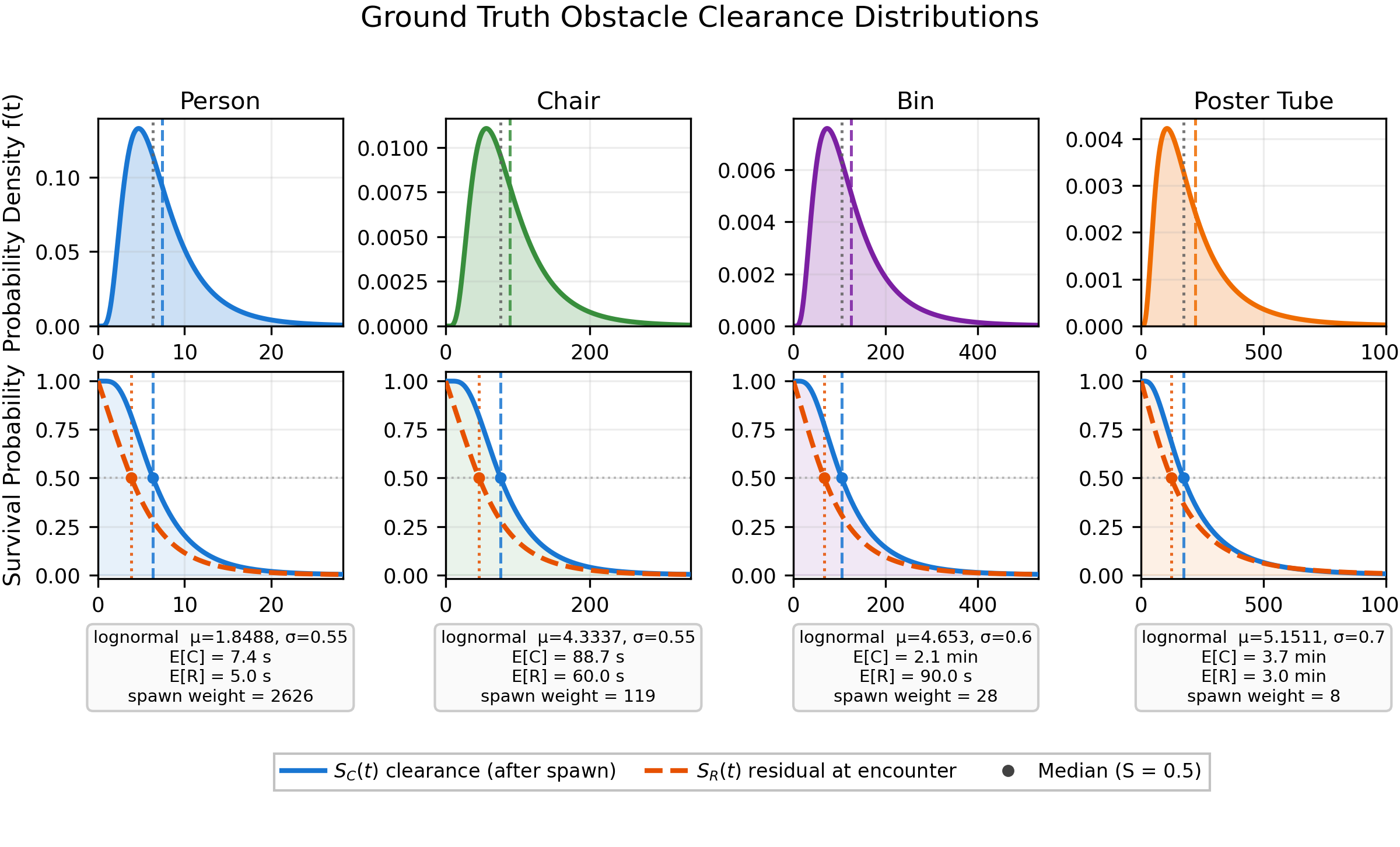
Each class has a lognormal lifetime from spawn, with people shorter-lived and tubes longest-lived. An obstacle encountered at a random steady-state time is length-biased: longer-lived obstacles are more likely to be present. The relevant residual survival is the normalized integral of the original lifetime survival, not that raw lifetime curve. The robot learns this remaining-time distribution directly from encounters.
Equations
Appendix B.2 Poisson Obstacle Spawning
A global Poisson process chooses spawn locations uniformly; attempts on an occupied edge are ignored. Each edge alternates free and blocked periods. The rate is selected so mean blocked time divided by mean cycle time equals the desired occupancy, using five percent in the main setting. A 1,500-second warm-up brings the field toward stationarity before navigation begins.
Equations
Appendix B.3 Class Spawn Weights
Encountered class frequencies weight spawn frequencies by mean lifetime. To target a 55/30/10/5 percent encounter mix, the appendix uses approximately 94.4/4.3/1.0/0.3 percent spawn probabilities for person/chair/bin/tube. This differs from the main text’s statement that 55/30/10/5 are spawn probabilities. The appendix’s explicit lifetime-corrected construction is retained as the detailed protocol.
Equations
Appendix B.4 Learning and Planning Settings
The learned policy starts without seeded clearance samples and updates once per completed episode, with no explicit exploration. This paragraph specifies 300 points for both patience and downstream time grids, a global 2,000-second cap, and class caps of 300 seconds for people and 1,000 for each other class. These settings differ in description from the event-time-only search in the main method. Initial empty-curve behavior and finite-tail conventions are not fully documented.
Equations
Appendix B.5 Episodes, Timeouts, and Baselines
Episodes exceeding 3,600 seconds count as failures and receive that full duration in time statistics. One hundred seeds each run one thousand episodes. Greedy CTP permanently excludes observed blocked edges for the rest of the episode, which can disconnect the effective graph; its poor timeout-dominated result should be interpreted against this specific heuristic, not all planners for the Canadian Traveller Problem.
Appendix B.6 Scenario Manifests for Real-World Experiments
Scenario manifests specify obstacle class, location, and timing for later physical runs. Logs from one run update survival estimates before the next manifest is used. This permits controlled reconstruction of traffic events and explains why the main physical evaluation is orchestrated.
Appendix B.7 Generalization Across Graph Topologies and Blockage Rates
Three graph topologies and blockage rates of two, five, and ten percent test different detour costs. Results use the final one hundred episodes of ten seeds. At ten percent on the original graph, OSCAR takes 268.8 seconds versus 311.2 for waiting and 512.5 for immediate rerouting. On a warehouse graph, expensive detours make waiting competitive with OSCAR; on a grid, cheap alternatives make immediate rerouting competitive at low occupancy. These results show adaptation to the tested cost structure rather than uniform dominance of every heuristic in every regime.
Appendix Appendix C Obstacle Classification Prompt
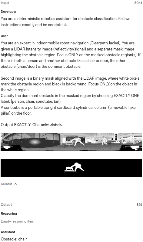
The complete original classifier prompt and deployment settings are preserved. The model receives a reflectivity image and, when available, a binary obstacle mask; it returns one fixed-format label from person, chair, bin, and sonotube. A person beside an object is treated according to the prompt’s object-priority rule. The classifier supplies labels only—clearance-duration estimation is disabled and navigation decisions remain in the planner. Deterministic wording and a fixed schema do not guarantee correct or deterministic model outputs, especially when the mask is unavailable.
Developer:
You are a deterministic robotics assistant for obstacle classification.
Follow instructions exactly and be consistent.

User:
You are an expert in indoor mobile robot navigation (Clearpath Jackal).
You are given a LiDAR intensity image (reflectivity/signal) and a
separate mask image highlighting the obstacle region. Focus ONLY on the
masked obstacle region(s). If there is both a person and another
obstacle like a chair or door, the other obstacle (chair/door) is the
dominant obstacle.

Second image is a binary mask aligned with the LiDAR image, where white
pixels mark the obstacle region and black is background. Focus ONLY on
the object in the white region.

Classify the dominant obstacle in the masked region by choosing EXACTLY
ONE label: {person, chair, sonotube, bin}.
A sonotube is a portable upright cardboard cylindrical column (a movable
fake pillar) on the floor.

Output EXACTLY: Obstacle: <label>.
Appendix Appendix D Person/Chair-Only Real-World Results
A supplementary run uses naturally appearing people and chairs without prescribed removal timers. Waiting remains common for people, while chairs elicit more detours. Travel time later rises as obstacle counts increase, so the curve is not a controlled stationary learning comparison. Bin and sonotube labels in this run are classification errors, not additional present object types. This provides useful qualitative evidence outside the staged protocol while directly exposing perception limitations.
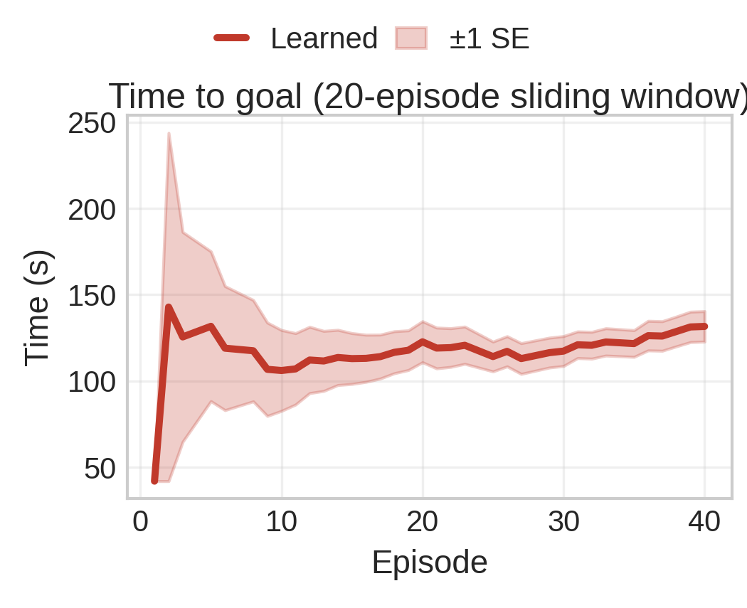
(a) Time-to-goal
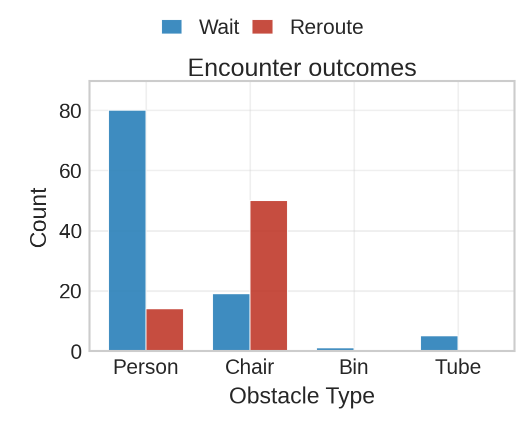
(b) Encounter outcomes
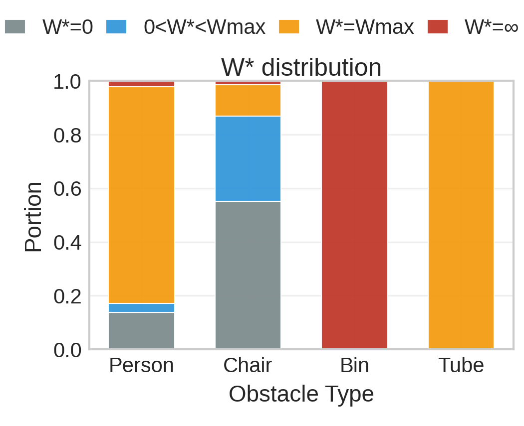
(c) Patience thresholds