Overview
Project resources. This edition follows the complete 33-page, 13 October 2026 v2, including seventeen figures, sixteen numbered tables, eleven equations and all 62 references.
At a glance
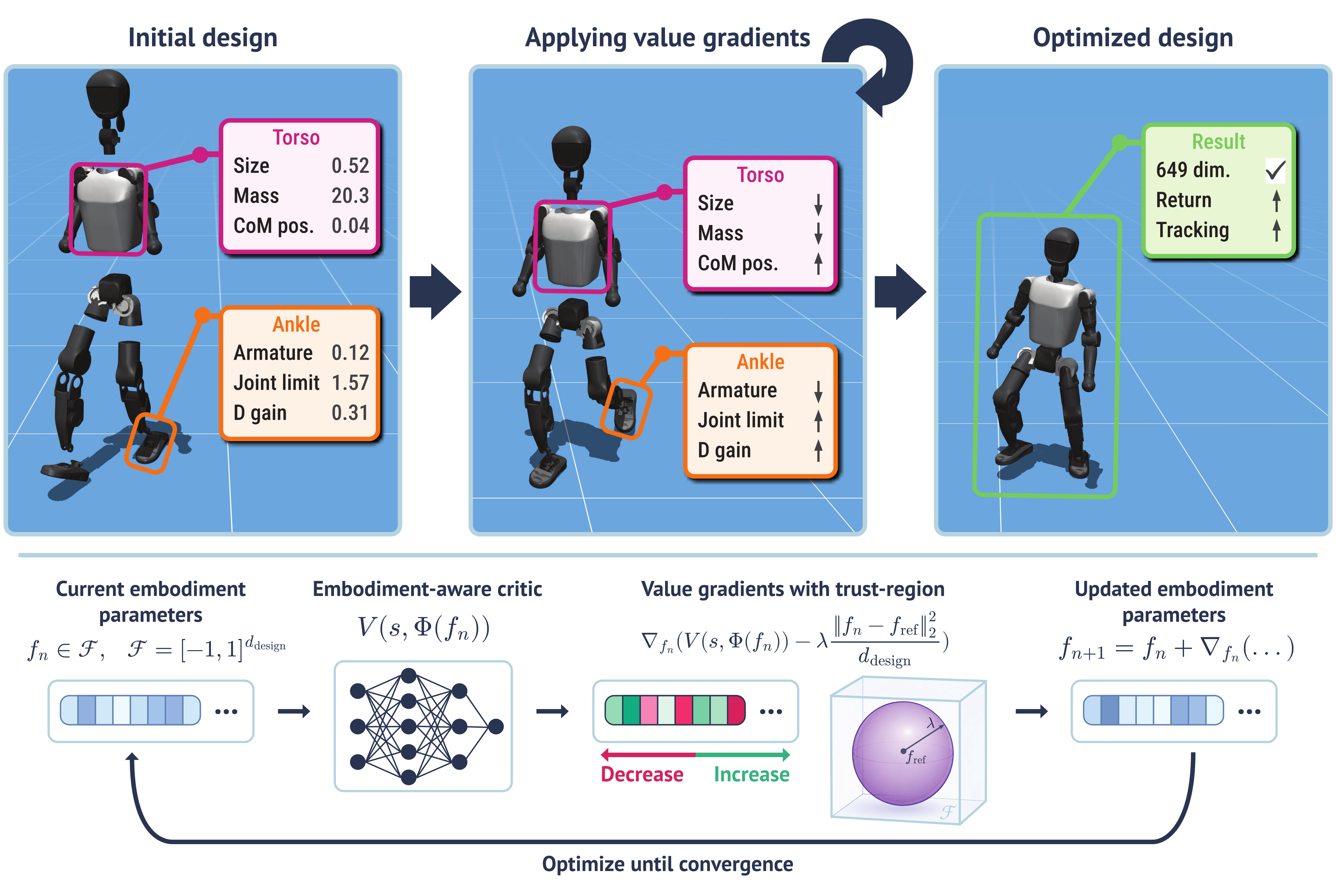
Shape Your Body trains an embodiment-aware locomotion policy and critic across randomized robots, then freezes both and differentiates the critic to optimize continuous design parameters. A penalty toward a reference design reduces exploitation of critic errors. Search improves many perturbed designs in simulation and can reuse one model across robots, but optimized hardware is neither manufactured nor tested; real deployments use the nominal robots.
1 Introduction
Robot co-design couples the body with its controller. Repeating control training for every candidate is expensive, so this work amortizes that cost through a generalist policy and value model. The frozen critic becomes a differentiable surrogate over masses, geometry, joint limits, actuation and control settings.
Experiments progress from randomized versions of one robot to a held-out robot within a morphology class, then a model trained on all fifty robots. The last setting includes the targets and is not held-out generalization. Gradients also identify groups of design changes; these should not automatically be interpreted as isolated causal importance.
2 Related Work
Early evolutionary morphology and automated robot design jointly searched bodies and behavior. Recent FEACRL, Transform2Act, BodyGen and Stackelberg PPO share experience across designs within a training run. Here a broad pretrained critic is reused for subsequent design problems.
URMA and embodiment scaling provide the multi-robot representation. Comparators include black-box optimizers and gradient-based GC-PFO, the strongest search baseline. The idea is also related to policy evaluation networks and explicit policy-conditioned value functions, which differentiate critics with respect to representations of what they evaluate.

3 Value Gradients for Multi-Embodiment Robot Design
A fixed-topology robot has physical parameters e=Φ(f), with normalized design f in [−1,1]ᵈ. Equation 1 defines discounted policy return; search aims to improve a candidate under a frozen embodiment-conditioned controller. It can alter geometry, dynamics, actuator limits and PD settings, but cannot add joints or change topology.
The differentiable map applies bounded transformations and consistency rules. These constrain the simulated model without certifying fabrication feasibility, real actuator availability or collision-free operation. Design-specific reward penalties are possible but are not added here.
Equation 1
| (1) |
3.1 Training a Multi-Embodiment Policy and Critic
At episode reset, sample a design from a curriculum-scaled box and hold it fixed for the rollout. PPO trains a shared policy. URMA encodes per-joint observations/descriptions, aggregates variable-length joint/foot information and produces per-joint actions or a scalar value.
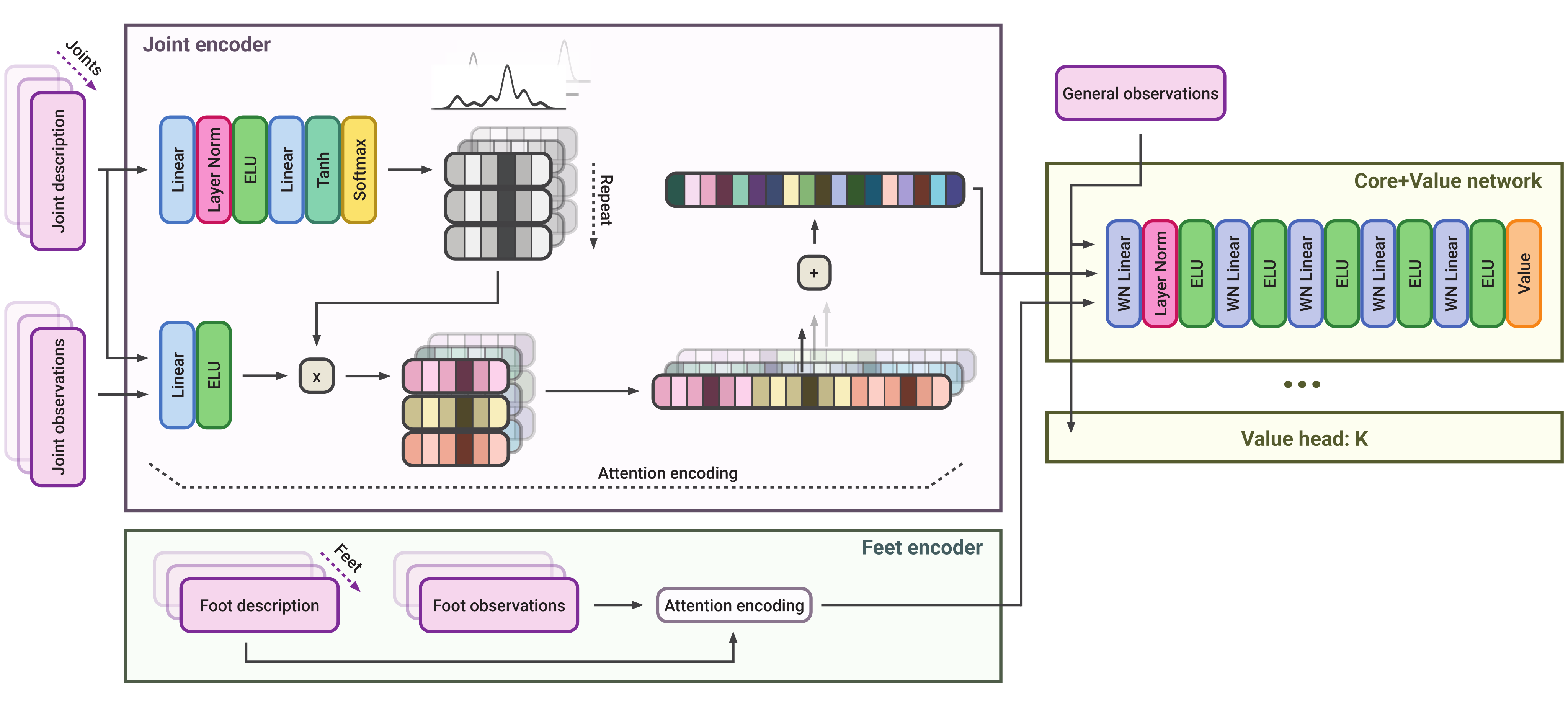
The direct-design critic feeds physical descriptions into attention values as well as keys, increasing design sensitivity. Three value heads share encoders and their mean drives search. This ensemble is not calibrated uncertainty: later tests show that heads can agree on harmful extrapolations.
Equations 2–3
| (2) |
| (3) |
3.2 Value-Gradient Design Search
Collect a fixed state bank under the trained policy, then maximize mean predicted value minus λ times average squared distance from a reference design. Equations 4–7 retain the ensemble, constrained formulation, soft penalty and clipped Adam update. Default search uses fifty iterations, learning rate 0.05, λ=100 and maximum normalized coordinate step 0.1.
These are derivatives of a learned surrogate, not exact gradients of rollout return. The fixed bank does not follow every candidate’s occupancy distribution. The soft penalty discourages extrapolation without imposing a hard radius; final clipping enforces the design box. Ablations support the recipe without establishing convergence or performance guarantees.
Equations 4–7
| (4) |
| (5) |
| (6) |
| (7) |
4 Experiments
The task tracks random planar-linear and yaw-velocity commands in RL-X with MuJoCo/MJX. Training spans fifteen quadrupeds, 31 bipeds/humanoids and four hexapods. Main results report return improvement from perturbed starts; Appendix I separately measures planar tracking-error reduction, which need not improve whenever the multi-term return does.
4.1 Single-Robot Design
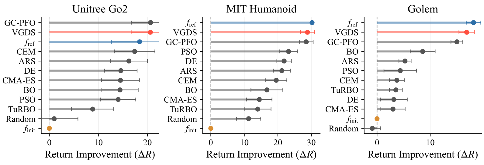
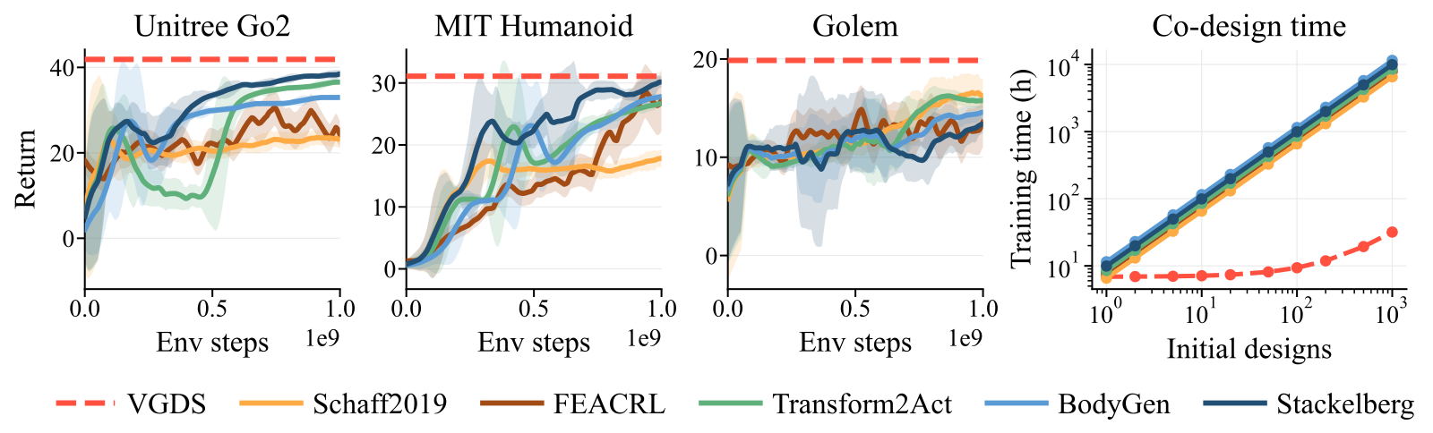
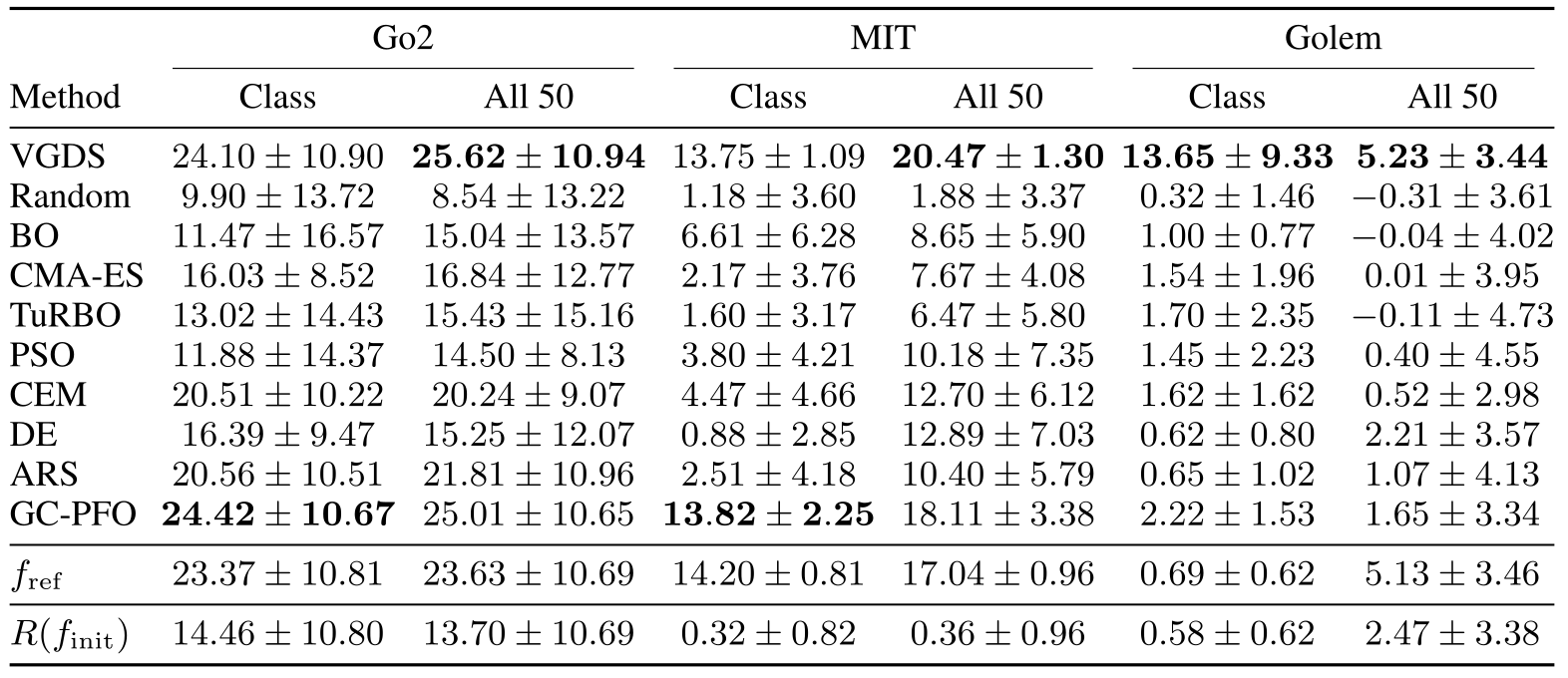
Separate models train on randomized Go2, MIT Humanoid and Golem designs with 358, 514 and 688 parameters. Ten starts per robot are searched with the same critic objective. VGDS approximately matches GC-PFO on Go2/MIT and improves Golem most. At λ=100, mean return gains are 20.60, 28.84 and 16.85.
The nominal anchor accounts for much of this recovery: following only the reference penalty gives 19.60, 27.97 and 16.35. The gain over random designs is therefore not all critic guidance. Adapted RL co-design baselines retrain for each start; reuse adds one to two minutes per design after seven to nine hours of single-robot training. The fifty-robot run costs about 2.5 days, excluded from that small marginal search cost.
4.2 Generalization Across Training Distributions
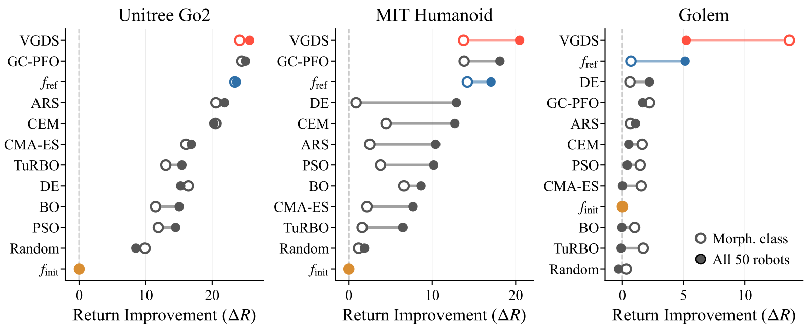
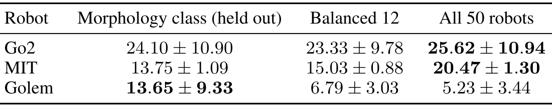
Class-specific training excludes the target; all-fifty training includes it. VGDS return gains with all fifty are 25.62 for Go2, 20.47 for MIT and 5.23 for Golem, versus held-out class gains 24.10, 13.75 and 13.65. GC-PFO slightly exceeds VGDS on held-out Go2/MIT (24.42/13.82), so there is no strict win in every cell.
Broader training benefits common classes but not Golem. The balancing study changes diversity and per-robot exposure too, so it does not isolate class count. Policies also have different initial/nominal returns: larger improvement across training sets need not mean higher absolute final performance.
4.3 Design Analysis with Value Gradients
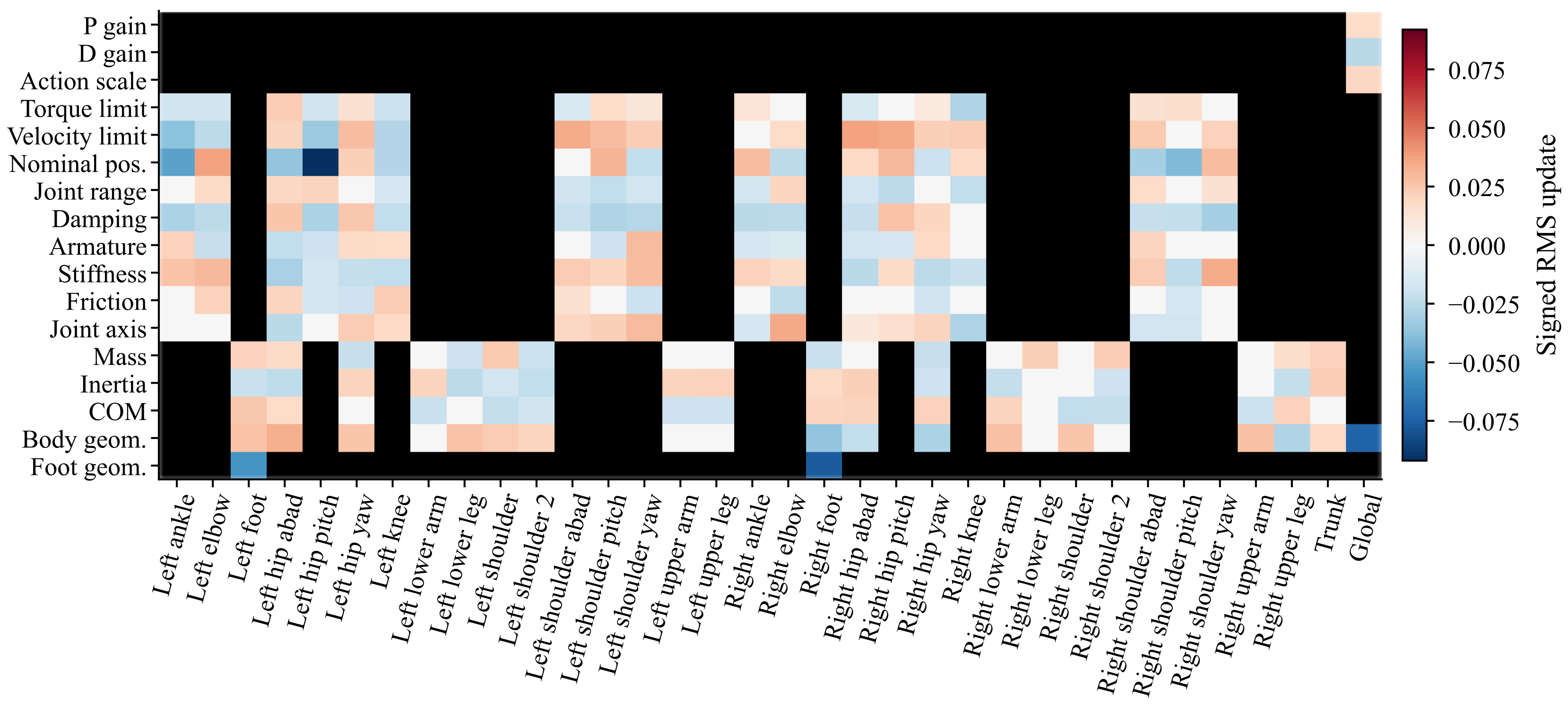
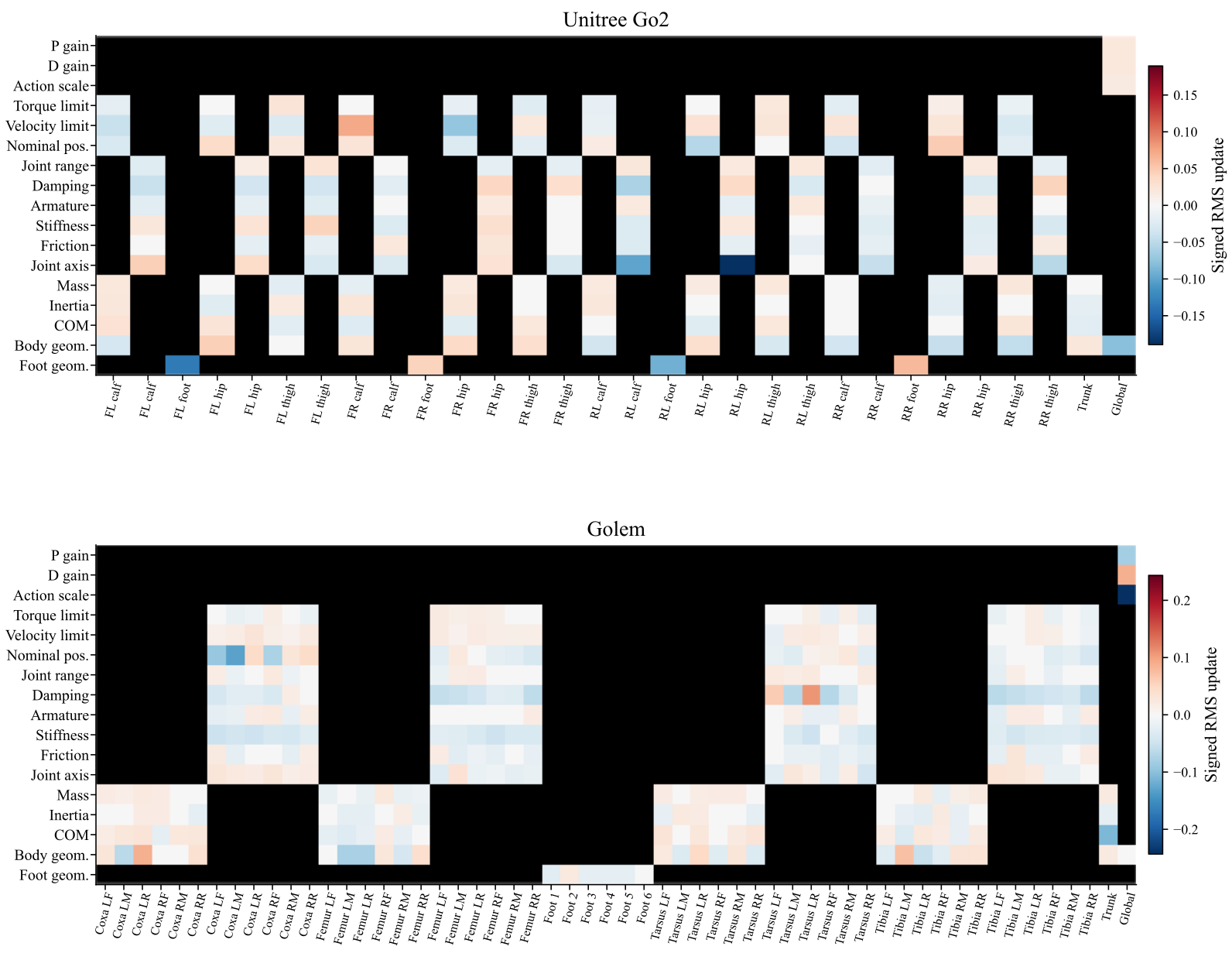
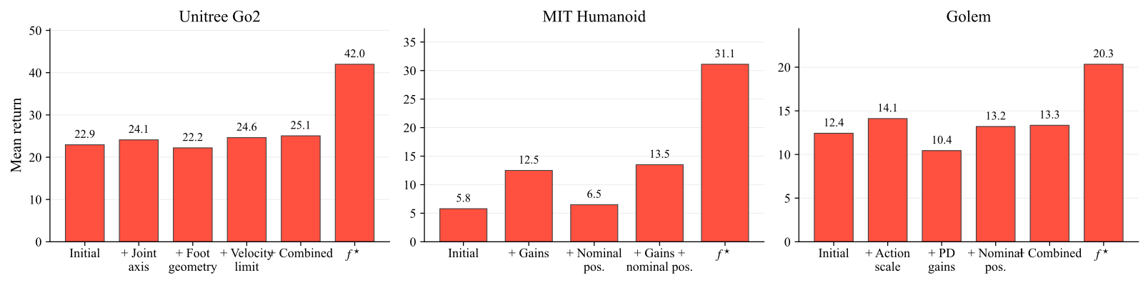
MIT changes emphasize nominal joint poses, gains and foot size: gains alone raise return 5.8→12.5, versus 31.1 for the full design. Go2 changes leg axes, foot geometry and actuator limits. Golem lowers action scale/P gain and raises D gain, although copying its gain changes alone hurts performance.
These coupled interventions support useful analysis, not a unique causal ranking. Some humanoids become shorter and wider; the proposed stability/training-distribution explanation is not separately established.
5 Limitations
Topology is fixed, and results depend on critic coverage, a useful reference and a controller capable of the candidate body. Comparatively simple simulations do not establish manufacturability or hardware transfer of optimized designs. Physical demonstrations validate only nominal robots. Materials, electronics, actuation and fabrication constraints remain open.
6 Conclusion
Embodiment-aware critics make high-dimensional design search inexpensive after training and help analyze combined body/control changes. The evidence is simulated improvement under frozen controllers, with strong dependence on the reference and surrogate. Proposed extensions include topology search, richer physical constraints/objectives and latent-space trust regions.
Acknowledgments
Funding is acknowledged from Poland’s National Science Centre Weave programme, UMO-2021/43/I/ST6/02711, and the German Research Foundation under PE 2315/17-1.
Appendix
Appendix A Experimental Setup Details
A.1 Environment
The JAX/MJX environment simulates at 200 Hz and controls at 50 Hz for at most twenty seconds or 1,000 actions. Early termination starts at 80% of nominal root height and relaxes toward zero with the curriculum. Robot-scale adjustments share the remaining task setup.
Actions and PD controller.
Equation 8 adds a robot-scaled action in [−10,10] to each nominal joint position; a PD controller tracks the target. Gains and action scale are searchable, so optimized embodiments include controller settings.
Equation 8
| (8) |
Observations and descriptions.
Joint observations include position offset, velocity, previous action and nominal-pose indicators. Descriptions encode axes, limits, gains, masses, inertias, geometry and global properties. Foot contacts/timing, linear velocity, terrain height and curriculum state are privileged critic inputs; the policy has a more restricted observation set.
A.2 Reward function
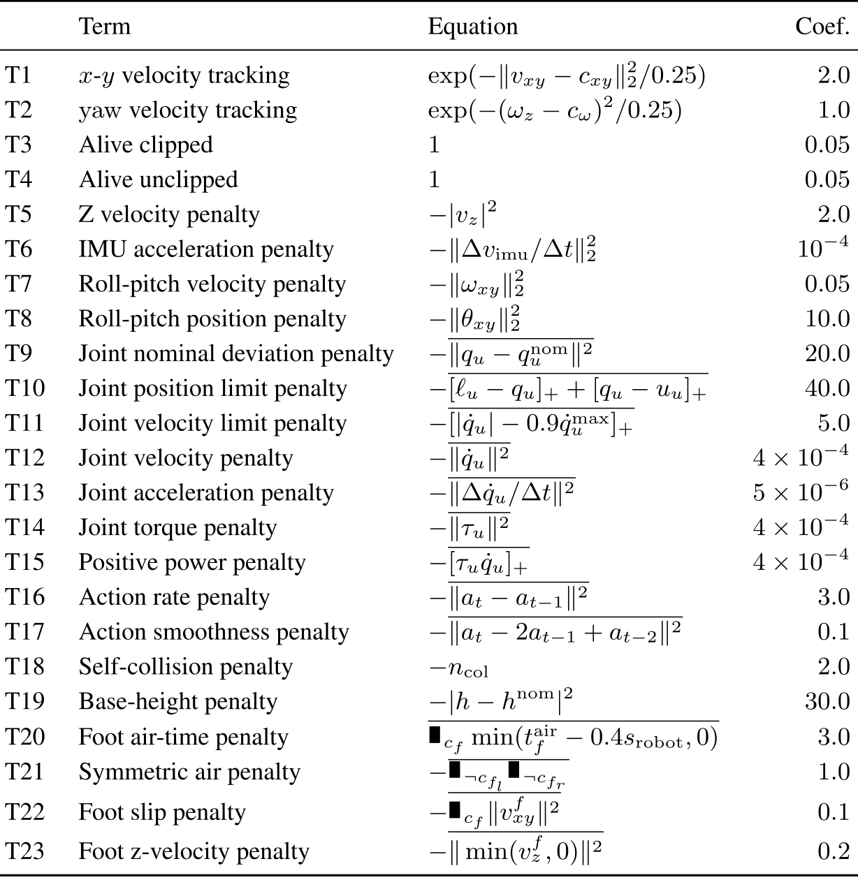
Equations 9–10 and Table 1 retain all 23 terms: planar/yaw tracking, survival and motion/effort/contact/joint penalties. Pre-reward is clipped below at zero before adding an unclipped survival term; coefficients scale with the control timestep. Return gains can trade tracking against other objectives.
Equations 9–10
| (9) |
| (10) |
Original selectable table
| Term | Equation | Coef. | |
|---|---|---|---|
| T1 | - velocity tracking | ||
| T2 | velocity tracking | ||
| T3 | Alive clipped | ||
| T4 | Alive unclipped | ||
| T5 | Z velocity penalty | ||
| T6 | IMU acceleration penalty | ||
| T7 | Roll-pitch velocity penalty | ||
| T8 | Roll-pitch position penalty | ||
| T9 | Joint nominal deviation penalty | ||
| T10 | Joint position limit penalty | ||
| T11 | Joint velocity limit penalty | ||
| T12 | Joint velocity penalty | ||
| T13 | Joint acceleration penalty | ||
| T14 | Joint torque penalty | ||
| T15 | Positive power penalty | ||
| T16 | Action rate penalty | ||
| T17 | Action smoothness penalty | ||
| T18 | Self-collision penalty | ||
| T19 | Base-height penalty | ||
| T20 | Foot air-time penalty | ||
| T21 | Symmetric air penalty | ||
| T22 | Foot slip penalty | ||
| T23 | Foot z-velocity penalty |
A.3 Curriculum and design sampling
The box expands from the nominal design to the full normalized range using the performance-based embodiment curriculum. Evaluation uses the full box. Training also perturbs observations and initial states, applies pushes and mixes action delays up to one control step.
A.4 Robots and design dimensions
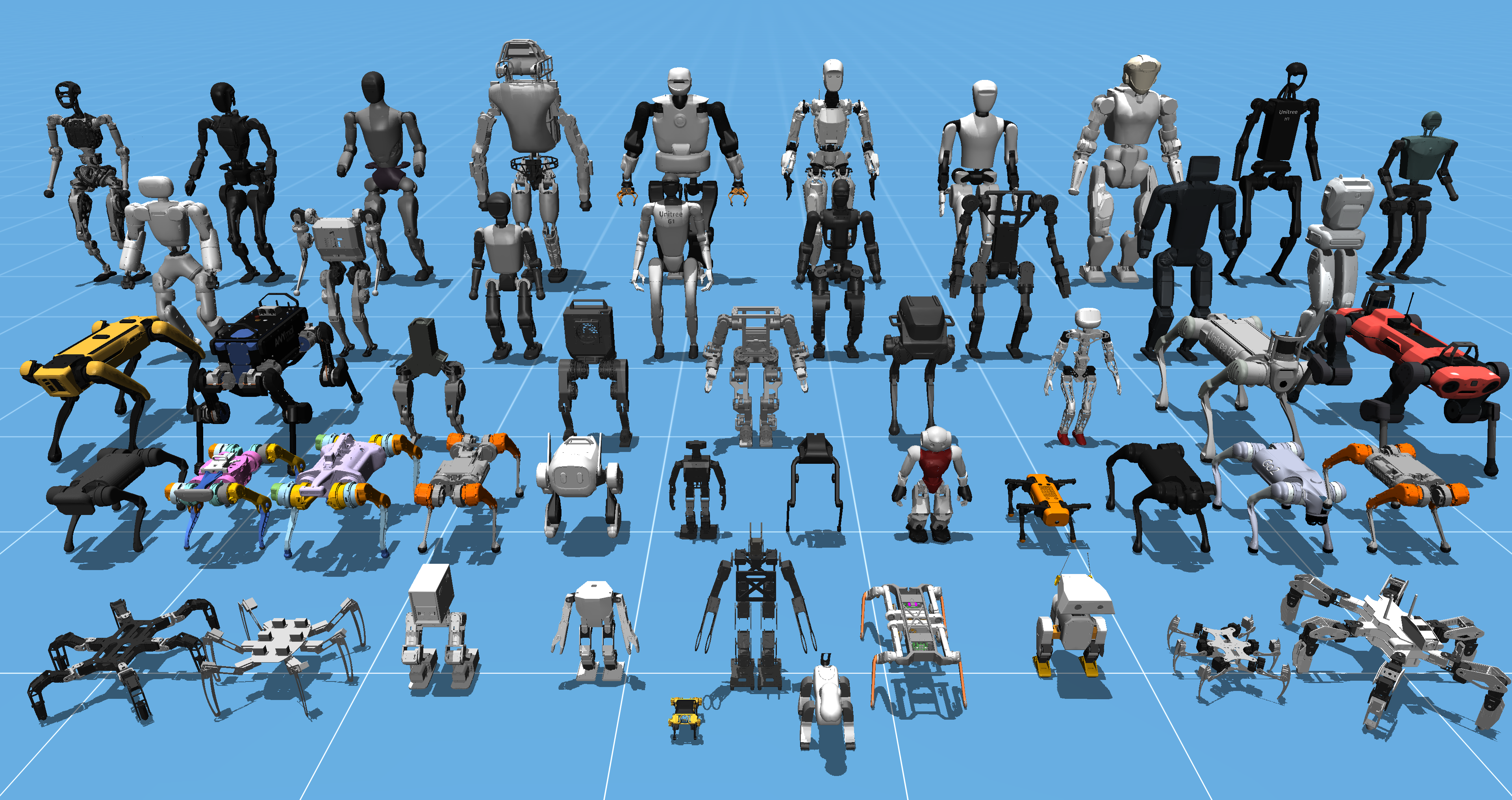
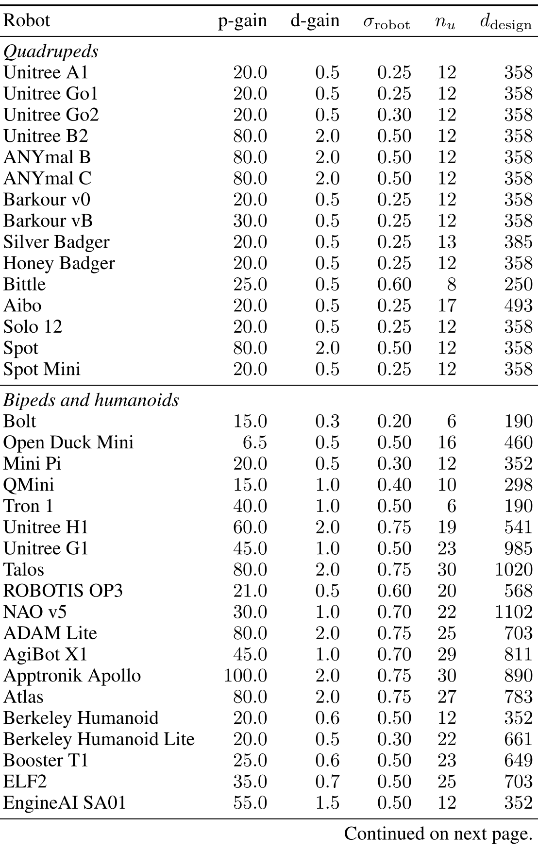
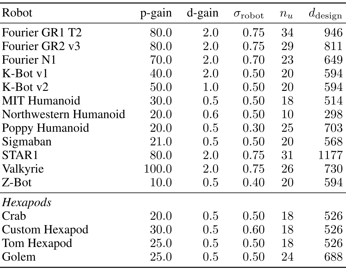
Figure 7 and the complete two-page Table 2 retain all fifty robots, gains, action scales, actuator counts and dimensions. STAR1 has the largest listed space, 1,177 parameters. Every robot keeps its kinematic topology.
Original selectable table
| Robot | p-gain | d-gain | |||
|---|---|---|---|---|---|
| Quadrupeds | |||||
| Unitree A1 | |||||
| Unitree Go1 | |||||
| Unitree Go2 | |||||
| Unitree B2 | |||||
| ANYmal B | |||||
| ANYmal C | |||||
| Barkour v0 | |||||
| Barkour vB | |||||
| Silver Badger | |||||
| Honey Badger | |||||
| Bittle | |||||
| Aibo | |||||
| Solo 12 | |||||
| Spot | |||||
| Spot Mini | |||||
| Bipeds and humanoids | |||||
| Bolt | |||||
| Open Duck Mini | |||||
| Mini Pi | |||||
| QMini | |||||
| Tron 1 | |||||
| Unitree H1 | |||||
| Unitree G1 | |||||
| Talos | |||||
| ROBOTIS OP3 | |||||
| NAO v5 | |||||
| ADAM Lite | |||||
| AgiBot X1 | |||||
| Apptronik Apollo | |||||
| Atlas | |||||
| Berkeley Humanoid | |||||
| Berkeley Humanoid Lite | |||||
| Booster T1 | |||||
| ELF2 | |||||
| EngineAI SA01 | |||||
| Fourier GR1 T2 | |||||
| Fourier GR2 v3 | |||||
| Fourier N1 | |||||
| K-Bot v1 | |||||
| K-Bot v2 | |||||
| MIT Humanoid | |||||
| Northwestern Humanoid | |||||
| Poppy Humanoid | |||||
| Sigmaban | |||||
| STAR1 | |||||
| Valkyrie | |||||
| Z-Bot | |||||
| Hexapods | |||||
| Crab | |||||
| Custom Hexapod | |||||
| Tom Hexapod | |||||
| Golem | |||||
A.5 PPO Training
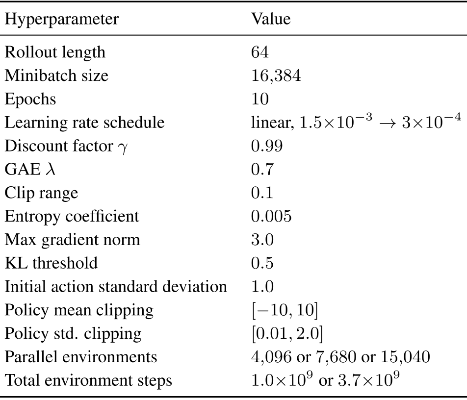
PPO uses 64-step rollouts, 16,384-sample minibatches, ten epochs, discount 0.99, GAE λ=0.7 and clip range 0.1. Single-robot training uses 4,096 environments/one billion steps; class training 7,680/3.7 billion; all-fifty training 15,040/3.7 billion. Hardware varies; the largest run takes about 2.5 days on one RTX 6000 Ada.
Original selectable table
| Hyperparameter | Value |
|---|---|
| Rollout length | |
| Minibatch size | |
| Epochs | |
| Learning rate schedule | linear, |
| Discount factor | |
| GAE | |
| Clip range | |
| Entropy coefficient | |
| Max gradient norm | |
| KL threshold | |
| Initial action standard deviation | |
| Policy mean clipping | |
| Policy std. clipping | |
| Parallel environments | or or |
| Total environment steps | or |
A.6 Design space parameters
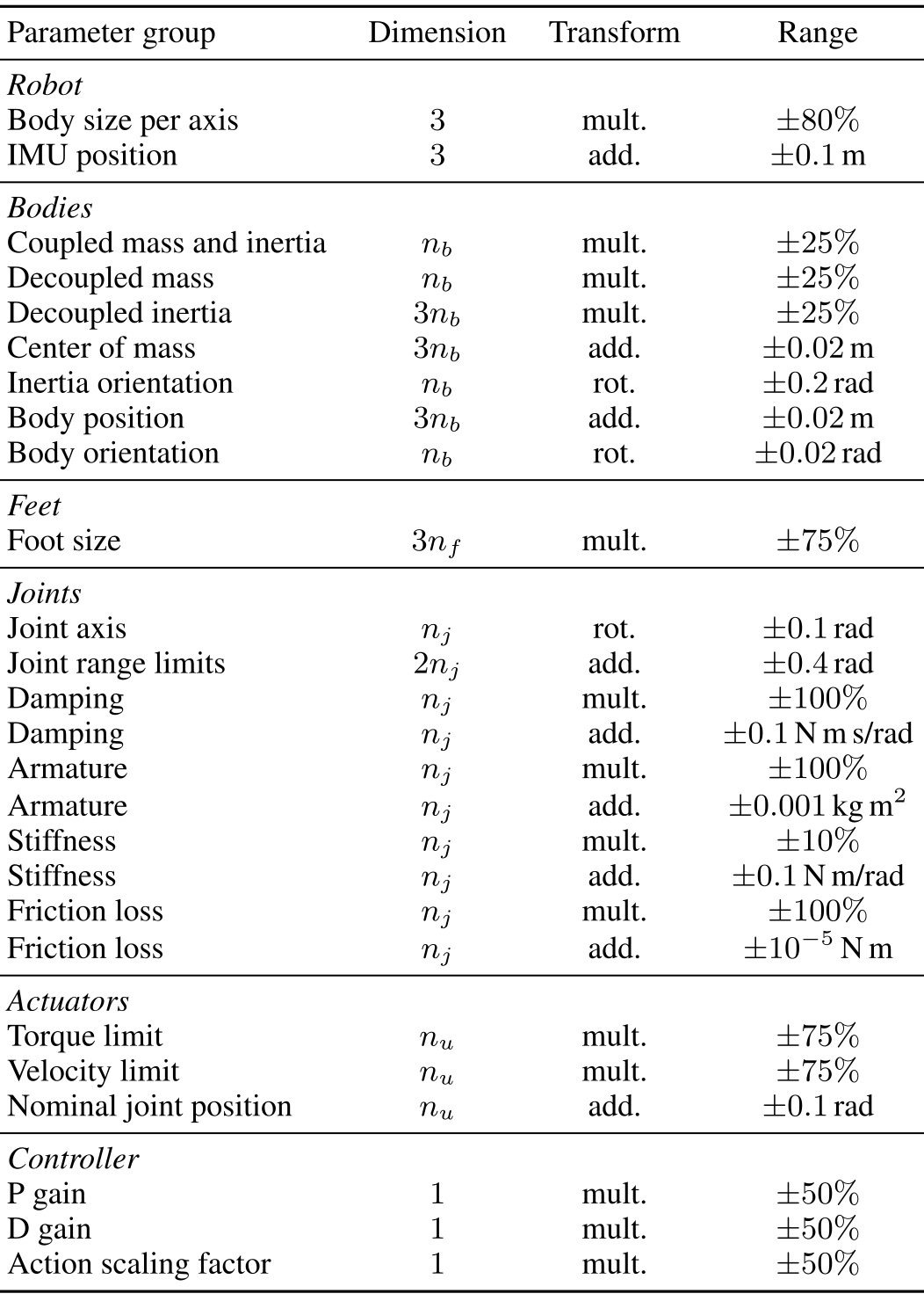
Table 4 gives every group, range and transform. Multiplicative groups use x=x_nom(1+κfᵢ); additive groups use x=x_nom+κfᵢ; rotations use fixed axes. For body/joint/actuator/foot counts n_b,n_j,n_u,n_f, dimension is 9+13n_b+11n_j+3n_u+3n_f.
Body-axis scaling also changes positions and derived mass/inertia/control properties; separate groups further vary masses and inertias. Damping, armature, stiffness and friction are nonnegative; nominal joint positions obey limits. Closed-loop robots disable body size, position and orientation changes. These are simulation constraints, not a complete engineering-feasibility certificate.
Original selectable table
| Parameter group | Dimension | Transform | Range |
|---|---|---|---|
| Robot | |||
| Body size per axis | mult. | ||
| IMU position | add. | m | |
| Bodies | |||
| Coupled mass and inertia | mult. | ||
| Decoupled mass | mult. | ||
| Decoupled inertia | mult. | ||
| Center of mass | add. | m | |
| Inertia orientation | rot. | rad | |
| Body position | add. | m | |
| Body orientation | rot. | rad | |
| Feet | |||
| Foot size | mult. | ||
| Joints | |||
| Joint axis | rot. | rad | |
| Joint range limits | add. | rad | |
| Damping | mult. | ||
| Damping | add. | N m s/rad | |
| Armature | mult. | ||
| Armature | add. | kg m2 | |
| Stiffness | mult. | ||
| Stiffness | add. | N m/rad | |
| Friction loss | mult. | ||
| Friction loss | add. | N m | |
| Actuators | |||
| Torque limit | mult. | ||
| Velocity limit | mult. | ||
| Nominal joint position | add. | rad | |
| Controller | |||
| P gain | mult. | ||
| D gain | mult. | ||
| Action scaling factor | mult. | ||
Appendix B Direct-Design URMA Critic
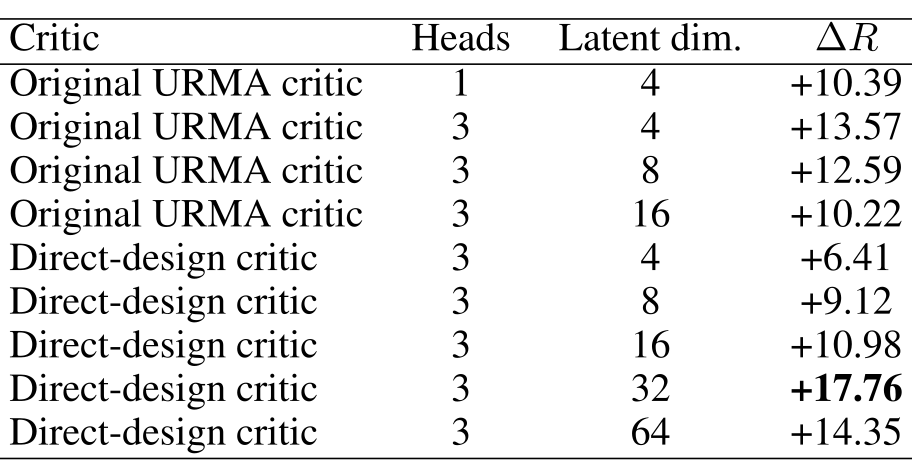
Descriptions enter the critic’s value encoders directly. A 32-dimensional joint-value latent with three heads gives +17.76 improvement in the early Go2 ablation, versus +13.57 for the original three-head critic at dimension four. Direct conditioning with four dimensions is worse (+6.41), and 64 dimensions falls to +14.35. Architecture and capacity both matter.
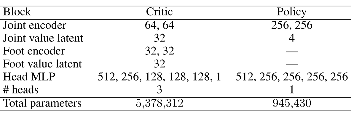
Figure 8 and Tables 5–6 retain the details: about 5.38 million critic and 0.95 million policy parameters. Shared heads use weight normalization. This small ablation does not establish universal superiority across robot distributions.
Original selectable table
| Critic | Heads | Latent dim. | |
|---|---|---|---|
| Original URMA critic | 1 | 4 | +10.39 |
| Original URMA critic | 3 | 4 | +13.57 |
| Original URMA critic | 3 | 8 | +12.59 |
| Original URMA critic | 3 | 16 | +10.22 |
| Direct-design critic | 3 | 4 | +6.41 |
| Direct-design critic | 3 | 8 | +9.12 |
| Direct-design critic | 3 | 16 | +10.98 |
| Direct-design critic | 3 | 32 | +17.76 |
| Direct-design critic | 3 | 64 | +14.35 |
Original selectable table
| Block | Critic | Policy |
|---|---|---|
| Joint encoder | 64, 64 | 256, 256 |
| Joint value latent | 32 | 4 |
| Foot encoder | 32, 32 | — |
| Foot value latent | 32 | — |
| Head MLP | 512, 256, 128, 128, 128, 1 | 512, 256, 256, 256, 256 |
| # heads | 3 | 1 |
| Total parameters |
Appendix C Surrogate Optimizer Hyperparameters
All methods optimize the same λ=100 frozen-critic objective with 64-state minibatches. Final designs receive two hundred evaluation rollouts. Hyperparameters were tuned on early versions of the three perturbed-robot tasks. Budgets are roughly comparable, not exactly equal in gradient, critic or simulator cost.
Value-Gradient Design Search.
VGDS applies fifty Adam ascent steps at learning rate 0.05, clips each coordinate change to 0.1 and clips the design to [−1,1]. It returns the final iterate, not a certified global optimum.
Random search.
Random search scores 3,200 uniform designs and selects the highest surrogate objective, without rollout-based optimization feedback.
Bayesian optimization.
BO uses BoTorch SingleTaskGP, a Matérn kernel and qLogNoisyExpectedImprovement. Ten Sobol points include the start, followed by fifty iterations. Acquisition optimization uses eight restarts, 256 raw samples and one candidate per batch.
Covariance matrix adaptation evolution strategy.
CMA-ES uses diagonal covariance for fifty generations, initial standard deviation 0.5 and population 4+floor(3 ln d), reducing the high-dimensional covariance cost.
Trust-region Bayesian optimization.
The baseline labeled TuRBO is adaptive trust-region random search here: fifty rounds of 64 candidates, radius initially 0.1 with range 0.005–0.5, shrinking by 0.7 or expanding by 1.3. This is not a full reproduction of the original Bayesian-optimization method.
Particle swarm optimization.
Global-best PSO uses 32 particles for fifty iterations, with inertia 0.9, cognitive coefficient 0.5 and social coefficient 0.3.
Cross-entropy method.
CEM samples 32 particles for fifty iterations, refits a diagonal Gaussian to the best 20%, and uses initial/floor standard deviations 0.5/0.02.
Differential evolution.
DE uses 32 particles for fifty iterations, differential weight 0.5 and binomial-crossover probability 0.9. Trials replace particles only when the surrogate improves.
Augmented random search.
ARS uses sixteen antithetic finite-difference directions for fifty iterations, perturbation standard deviation 0.1 and learning rate 0.05, retaining all directions.
Gradient-covariance particle filter optimization.
GC-PFO uses two regions of 32 particles for fifty iterations. Objective-weighted resampling and gradient-covariance noise use step 0.2, temperature 1.0 and ε=10⁻⁸. It uses gradients and is not a derivative-free comparator.
Appendix D Trust-Region and Reference-Design Ablations
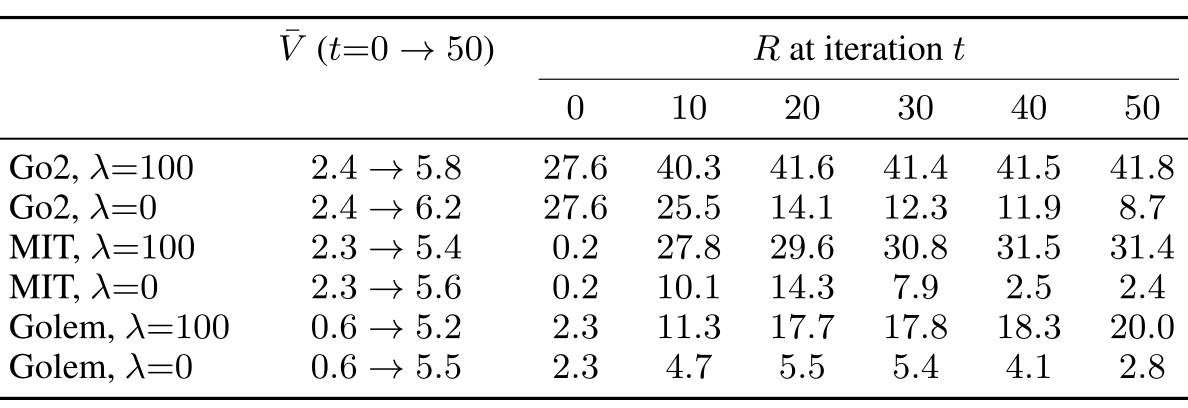
Without regularization, Go2 mean improvement is −18.93; λ=100 gives +20.60. MIT/Golem also benefit, although larger penalties give their best tested values. Penalty-only updates recover nearly as much as the full method, emphasizing the strong nominal anchor.
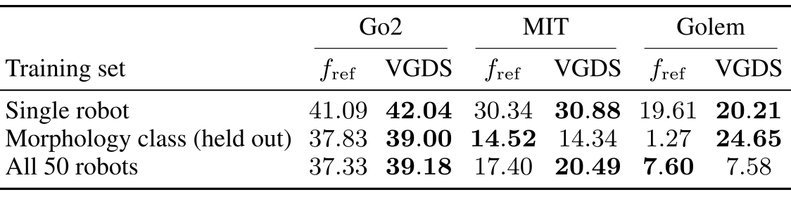
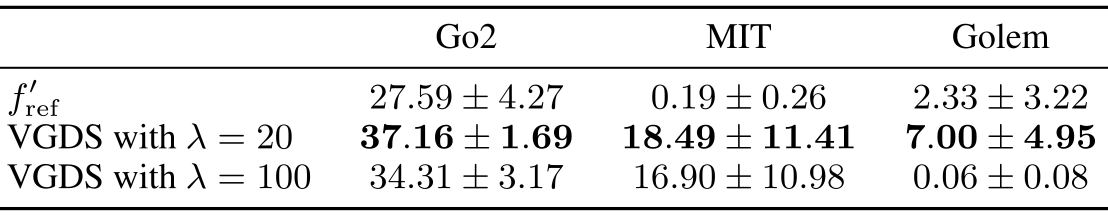
Starting at the nominal body improves most Table 8 settings, but held-out MIT falls 14.52→14.34 and all-robot Golem 7.60→7.58. With degraded anchors, λ=20 gives Go2/MIT/Golem returns 37.16/18.49/7.00; λ=100 worsens Golem from 2.33 to 0.06. Robustness to poor anchors is therefore conditional. Exact λ-invariance under Adam, asserted for penalty-only updates, also idealizes finite numerical ε; the reported ablation is the practical evidence.

Appendix E Critic Reliability Analysis
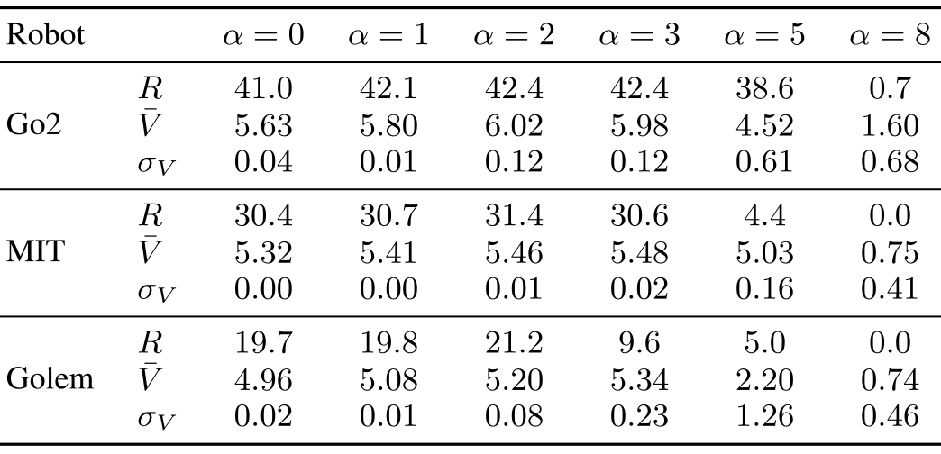
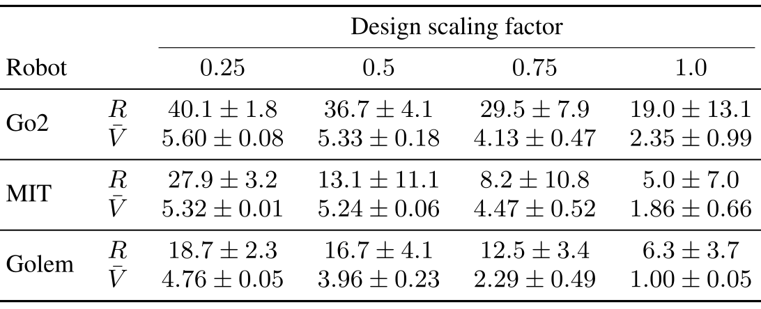
The critic can be exploited even when random-design averages look sensible. Scaling the found direction eventually destroys rollout return while value stays optimistic: MIT at α=5 returns 4.4 versus 30.7 at α=1. In unregularized Go2 search, return falls 27.6→8.7 while predicted value rises 2.4→6.2.
Head disagreement sometimes warns of failure, but Appendix O also reports confident catastrophic extrapolation. Three random samples per robot give limited evidence of average trends, not calibration guarantees. Discounted value and reported rollout return have different scales. Scaling α above one can leave the normal box; it is a stress test, not the bounded main search.
Original selectable table
| Robot | |||||||
|---|---|---|---|---|---|---|---|
| Go2 | |||||||
| MIT | |||||||
| Golem | |||||||
Original selectable table
| Design scaling factor | |||||
|---|---|---|---|---|---|
| Robot | |||||
| Go2 | |||||
| MIT | |||||
| Golem | |||||
Appendix F Policy Fine-Tuning at Optimized Designs
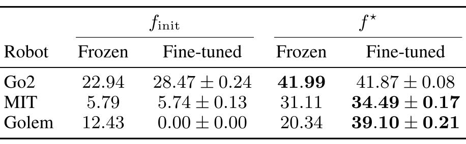
Fine-tuning for 52 million steps at the optimized body changes Go2 41.99→41.87, MIT 31.11→34.49 and Golem 20.34→39.10. Frozen policies can thus underestimate a design’s attainable performance. Fine-tuning initial Golem instead collapses 12.43→0.00. The absent Go2 gain is not proof of global policy optimality.
Original selectable table
| Robot | Frozen | Fine-tuned | Frozen | Fine-tuned |
|---|---|---|---|---|
| Go2 | ||||
| MIT | ||||
| Golem | ||||
Appendix G Class-Balanced Training Distribution
A balanced twelve-robot set includes four per class and the targets. Go2/MIT/Golem gains are 23.33/15.03/6.79, versus all-fifty 25.62/20.47/5.23. Held-out hexapod-only training reaches 13.65 for Golem but uses about 4.5 times more steps per robot. Balance, diversity, target inclusion and exposure remain entangled.
Original selectable table
| Robot | Morphology class (held out) | Balanced 12 | All 50 robots |
|---|---|---|---|
| Go2 | |||
| MIT | |||
| Golem |
Appendix H Sim-to-Real Transfer of the Training Pipeline
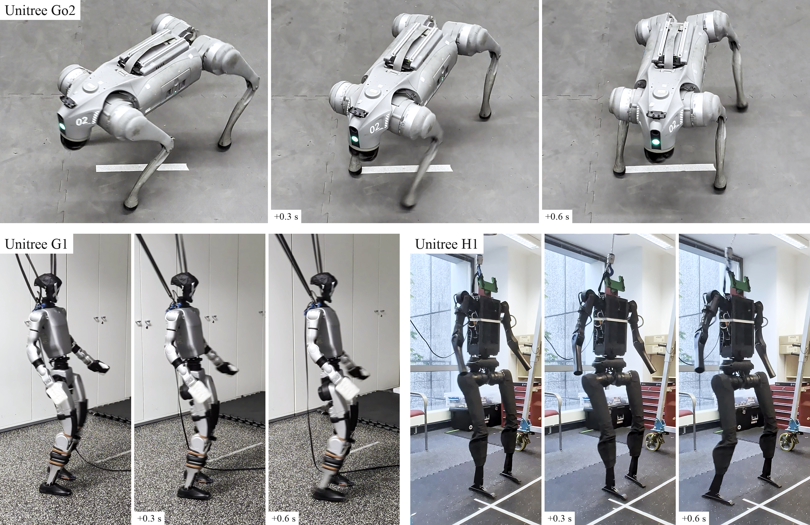
The all-fifty policy is deployed on nominal Unitree Go2, G1 and H1 for ordinary omnidirectional walking. Figure 9 documents qualitative transfer. No optimized body is manufactured/tested, and no quantitative hardware tracking comparison is supplied.
Appendix I Velocity Tracking Error Reduction Results
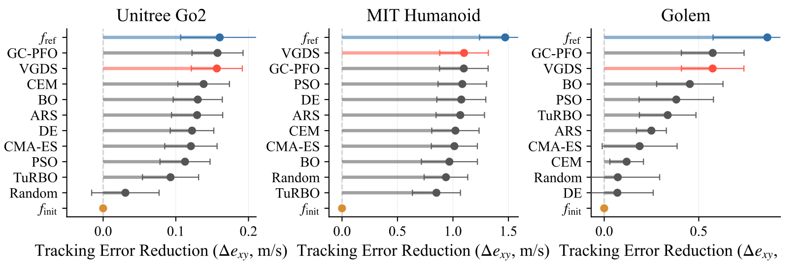
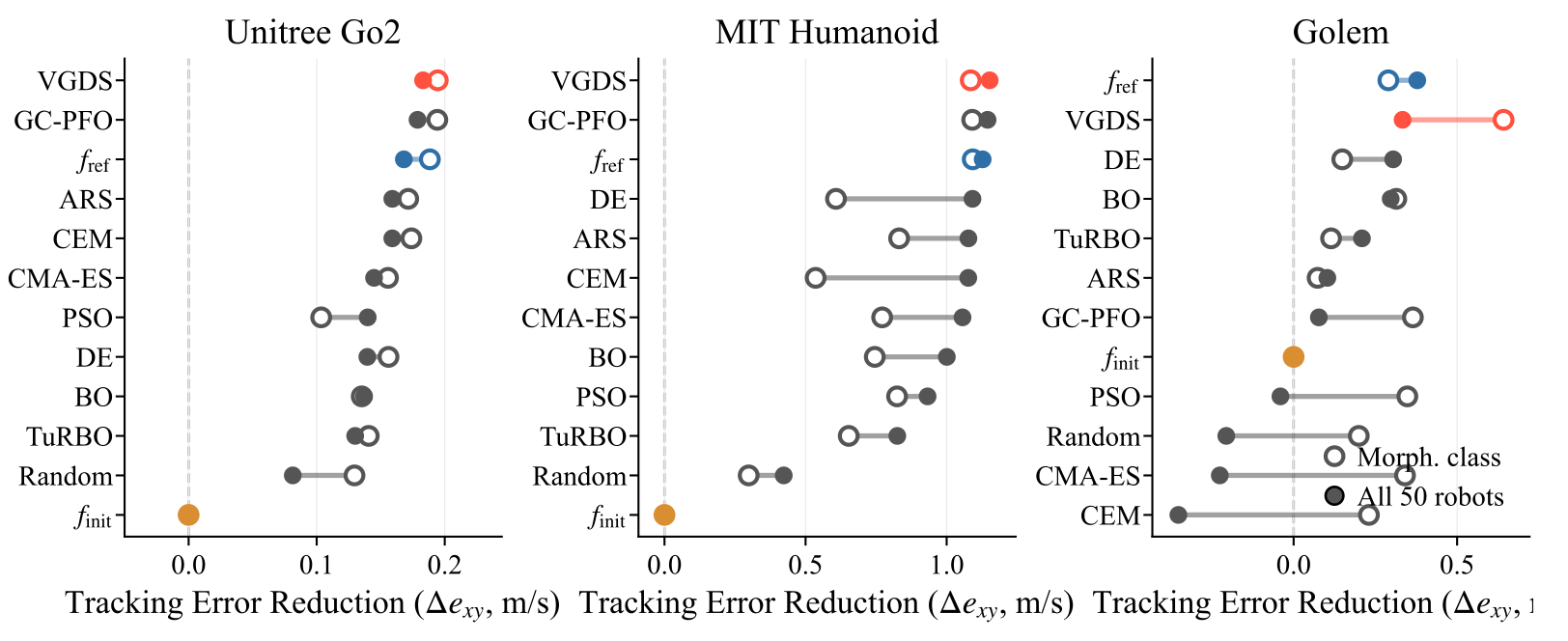
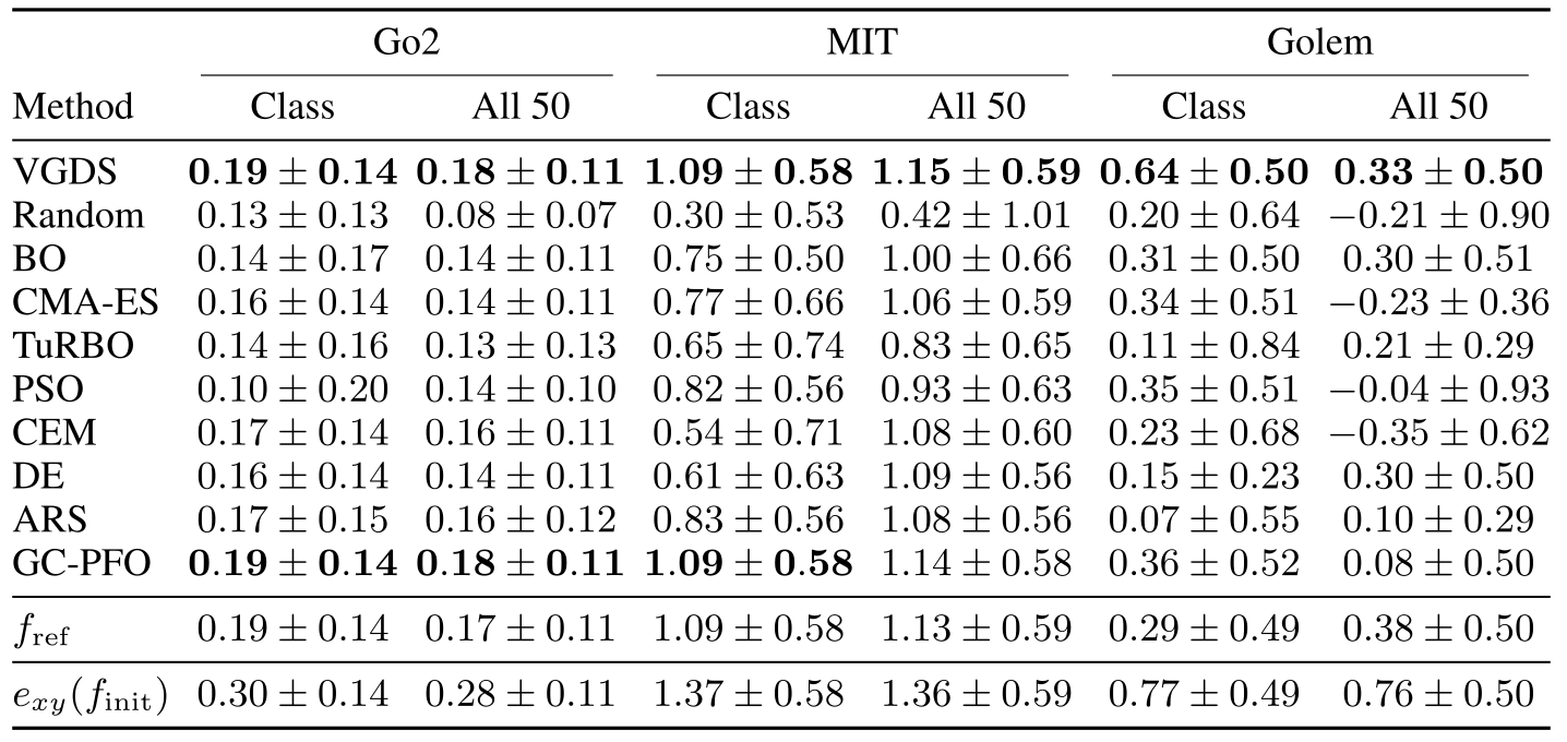
Equation 11 defines positive improvement as reduced absolute planar velocity error. VGDS and GC-PFO are similar on single-robot tasks. Training-set trends broadly follow return gains but differ in some rankings: multi-term return need not imply better tracking than the nominal body.
The Golem x-axis label in Figures 10–11 is truncated in both the published paper and its original web figure; the axis is tracking-error reduction in m/s, as defined above.
Equation 11
| (11) |
Appendix J Numeric Results for the Training Set Comparison
Tables 15–16 retain all means and standard deviations across ten starts. VGDS held-out/all-fifty tracking reductions are 0.19/0.18 m/s for Go2, 1.09/1.15 for MIT and 0.64/0.33 for Golem. Golem’s all-fifty nominal reference reduces error by 0.38, more than the optimized 0.33 despite a smaller return gain. Standard deviations are not paired significance tests.
Appendix K RL Co-Design Baselines
Five methods are substantially adapted to fixed-topology continuous design, URMA networks and on-policy PPO. Results compare these adaptations of the ideas, not faithful original implementations or their topology-search abilities.
Schaff2019.
Schaff2019 updates a population distribution over normalized designs using rollout returns while training a design-conditioned PPO controller. Environments sample from the current distribution.
Fast Evolutionary Actor-Critic Reinforcement Learning.
Original FEACRL uses off-policy SAC and an action-value critic. The adaptation substitutes PPO and state-value scoring over a start-state buffer, with PSO design selection, changing both learning and scoring.
Transform2Act.
Transform2Act proposes a continuous design update at episode start, followed by its execution policy. Both use PPO; discrete skeleton changes are removed.
BodyGen.
BodyGen retains stage-specific credit assignment and separate design/control critics. Its topology-aware self-attention is omitted in favor of fixed topology and URMA descriptions.
Stackelberg PPO.
Stackelberg PPO treats the design policy as leader and the adapting URMA/PPO controller as follower, within the same fixed-topology continuous space.
Appendix L All 50 Robots Design Results
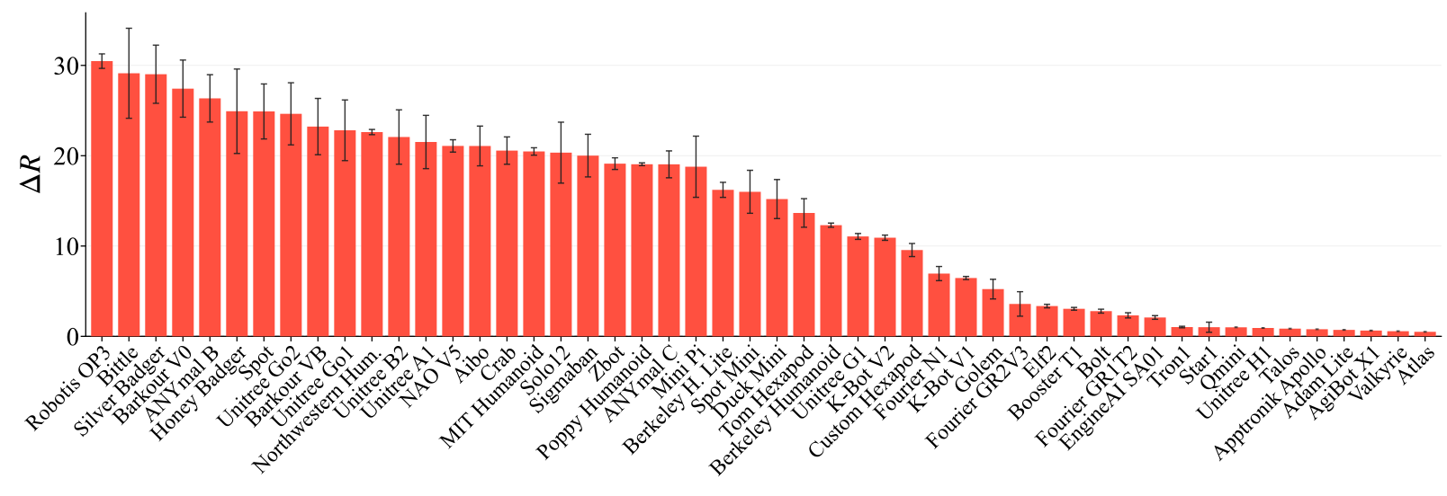
Figure 12 retains all fifty per-robot results, with ten random starts each. All are training-set robots. Some large humanoids have near-zero gains, attributed to incompletely converged controllers; no held-out-all-fifty generalization claim follows.
Appendix M Design Analysis Details
Signed RMS summarizes group changes relative to the reference. Selected substitutions recover only part of the gain: Go2 combined groups return 25.1 versus full-design 42.0; MIT gains alone 12.5 versus 31.1; Golem action scale 14.1 versus 20.3. Golem PD gains alone worsen the start to 10.4.
No final coordinate in thirty single-robot designs exceeds |fᵢ|=0.9; average normalized changes are 0.027–0.042. These runs are not simply saturating bounds, without implying optimality. Seventeen partial interventions have overall critic/return Spearman correlation 0.40. Stretched meshes can be rendering artifacts, but Golem still has up to eight self-collisions at the nominal pose. Zero Go2/MIT collisions at one pose does not certify collision-free motion.
Appendix N Design Search Trajectories
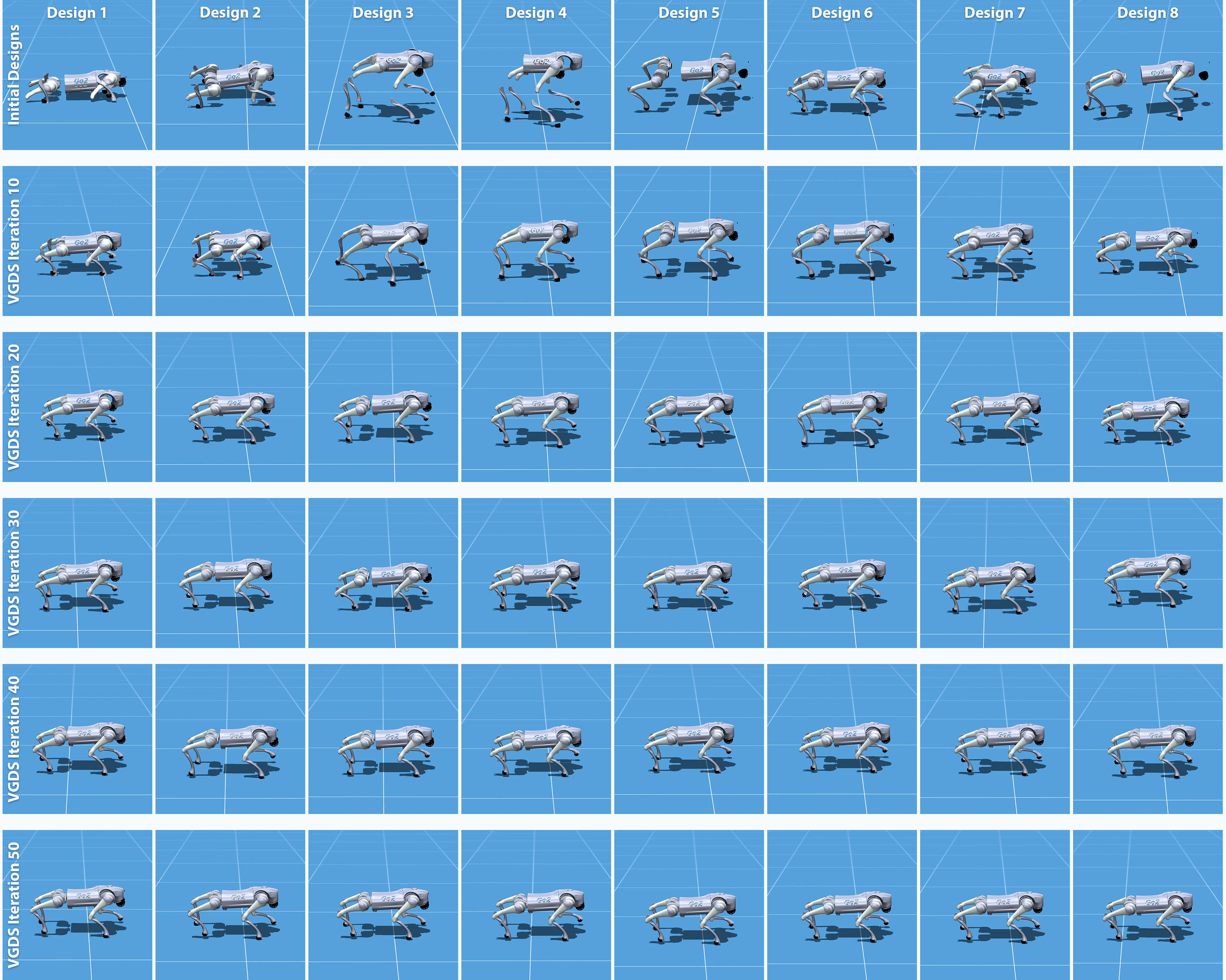
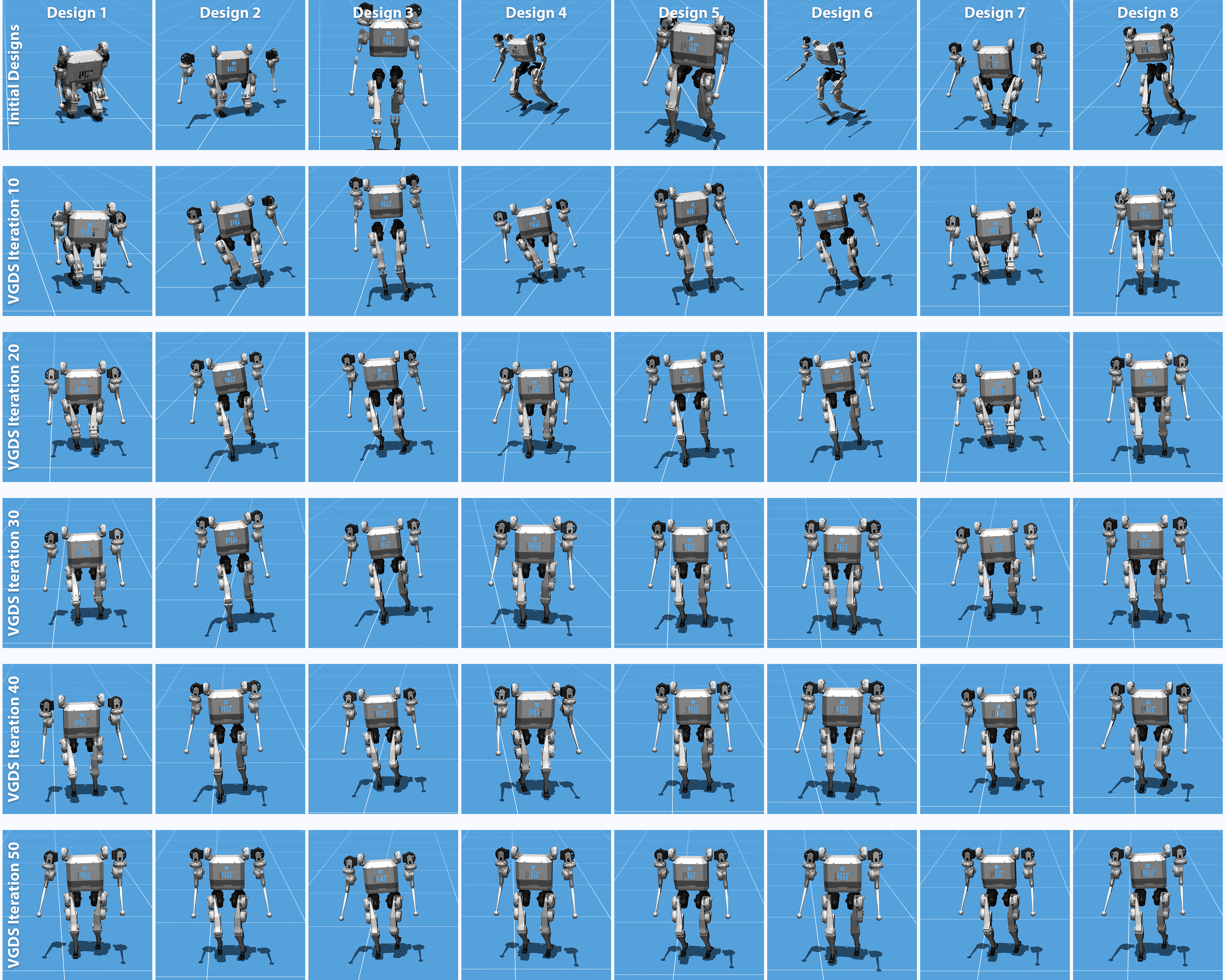
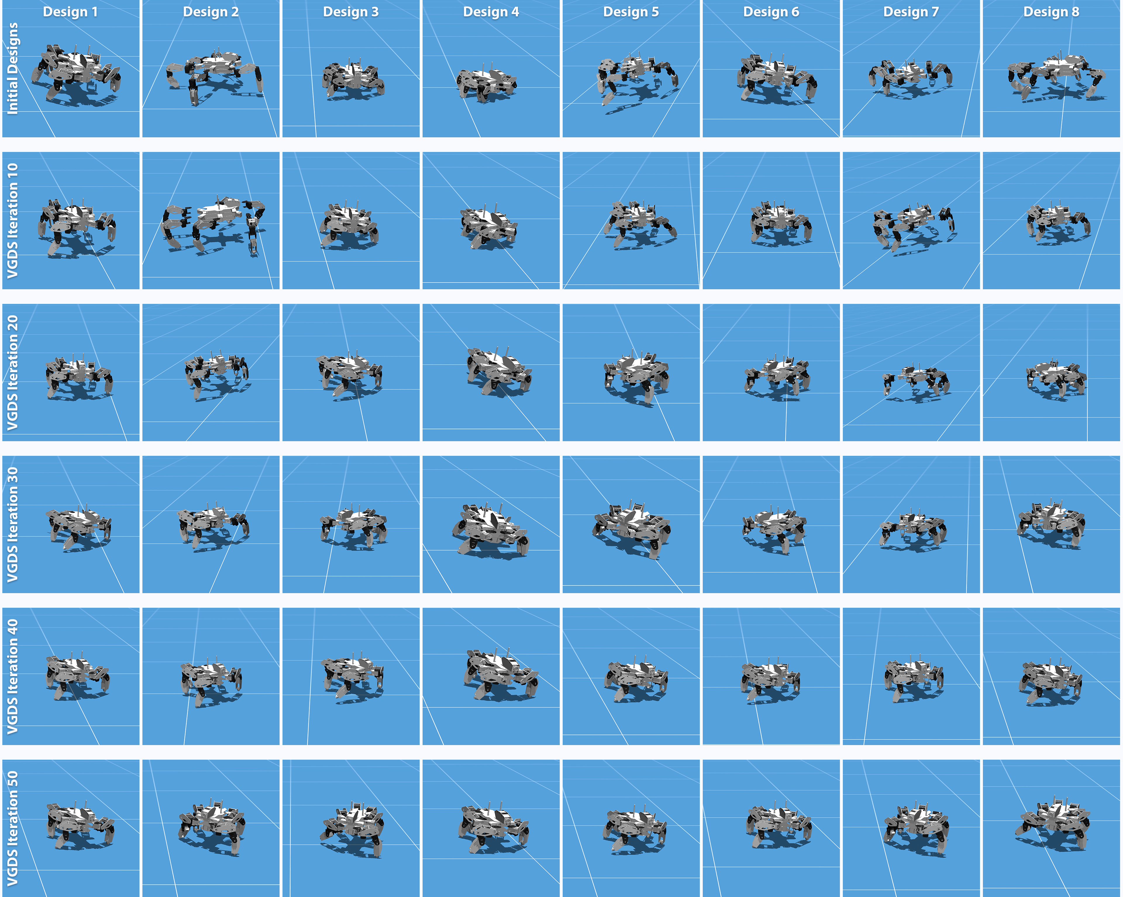
Figures 15–17 retain six stages for eight starts per robot, all 144 panels. Designs converge toward similar forms, reducing diversity. Fewer iterations, weaker penalties or lower learning rates are suggested trade-offs without a separate quantitative diversity study.
Appendix O Additional Method Variants
The appendix reports alternatives that did not consistently beat the chosen method, clarifying empirical design choices and failure modes.
Hard trust-region projection.
A hard-radius projection is competitive in some settings, but its radius proved harder to tune than the soft penalty. Both retain reference dependence.
Uncertainty-based trust regions.
Absolute/relative head disagreement and lower-confidence objectives fail as reliable reference-free trust regions: shared-data heads can agree on catastrophic extrapolation. Disagreement is a possible warning, not a safety certificate.
Search dynamics.
Noise, moment resets, norm clipping, cosine schedules, SGD and rate/step sweeps do not consistently improve the selected Adam configuration. More iterations can exploit critic errors further.
Multi-start search.
Nearby starting particles with surrogate-based selection do not consistently improve on one design once the penalty is tuned. This does not establish global optimality of single-start search.
Direction and subspace structure.
Restricting updates to large-gradient coordinates hurts. Removing one dominant direction is mostly harmless, while using only that direction collapses performance, suggesting useful updates are distributed across parameters.
Refreshing the state bank.
Refreshing the bank with current-design rollouts or initial states does not improve results and sometimes worsens them. Overlapping state distributions and a robust policy are the authors’ explanation, not proof of unbiased design-return gradients from fixed states.