At a glance
ViewSuite tests whether vision–language models can connect camera actions to changing images and plan toward a target viewpoint. Alternating reinforcement learning with supervised examples distilled from an accumulated view graph raises Qwen2.5-VL-7B interactive success from 2.5% to 47.8%, versus Gemini 3.1 Pro at 21.3%. The gain is substantial on this simulated indoor benchmark; the analyses do not establish that the model can reliably infer unseen viewpoints without approaching them.
1 Introduction
View planning couples action, observation and spatial localization: a camera move changes what evidence is available for the next decision. ViewSuite renders real ScanNet reconstructions, offers six-degree-of-freedom camera control and separates supplied-path tracking from interactive target localization. Table 1 places this setting alongside view reasoning and active-perception benchmarks.
Because initially successful rollouts are rare, terminal reward alone offers little learning signal. The proposed method stores even unsuccessful exploration in a graph and turns experienced transitions into attainable supervised tasks. It needs no stronger teacher model, but does use instrumented camera poses, rendered views and environment-derived labels. This edition follows all 39 pages of the 2 July 2026 v4, preserving thirteen figures, fifteen tables, three algorithms, four numbered equations and the appendix prompts. Resources: project, code, models and data.
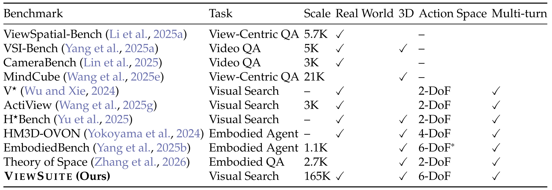
Original selectable table
| Benchmark | Task | Scale | Real World | 3D | Action Space | Multi-turn |
|---|---|---|---|---|---|---|
| ViewSpatial-Bench (Li et al., 2025a) | View-Centric QA | 5.7K | ✓ | – | ||
| VSI-Bench (Yang et al., 2025a) | Video QA | 5K | ✓ | ✓ | – | |
| CameraBench (Lin et al., 2025) | Video QA | 3K | ✓ | – | ||
| MindCube (Wang et al., 2025e) | View-Centric QA | 21K | ✓ | – | ||
| V⋆ (Wu and Xie, 2024) | Visual Search | – | ✓ | 2-DoF | ✓ | |
| ActiView (Wang et al., 2025g) | Visual Search | 3K | ✓ | 2-DoF | ✓ | |
| H⋆Bench (Yu et al., 2025) | Visual Search | – | ✓ | ✓ | 2-DoF | ✓ |
| HM3D-OVON (Yokoyama et al., 2024) | Embodied Agent | – | ✓ | ✓ | 4-DoF | ✓ |
| EmbodiedBench (Yang et al., 2025b) | Embodied Agent | 1.1K | ✓ | 6-DoF∗ | ✓ | |
| Theory of Space (Zhang et al., 2026) | Embodied QA | 2.7K | ✓ | 2-DoF | ✓ | |
| ViewSuite (Ours) | Visual Search | 165K | ✓ | ✓ | 6-DoF | ✓ |
2 ViewSuite : Problem Formulation, Environment, and Benchmark
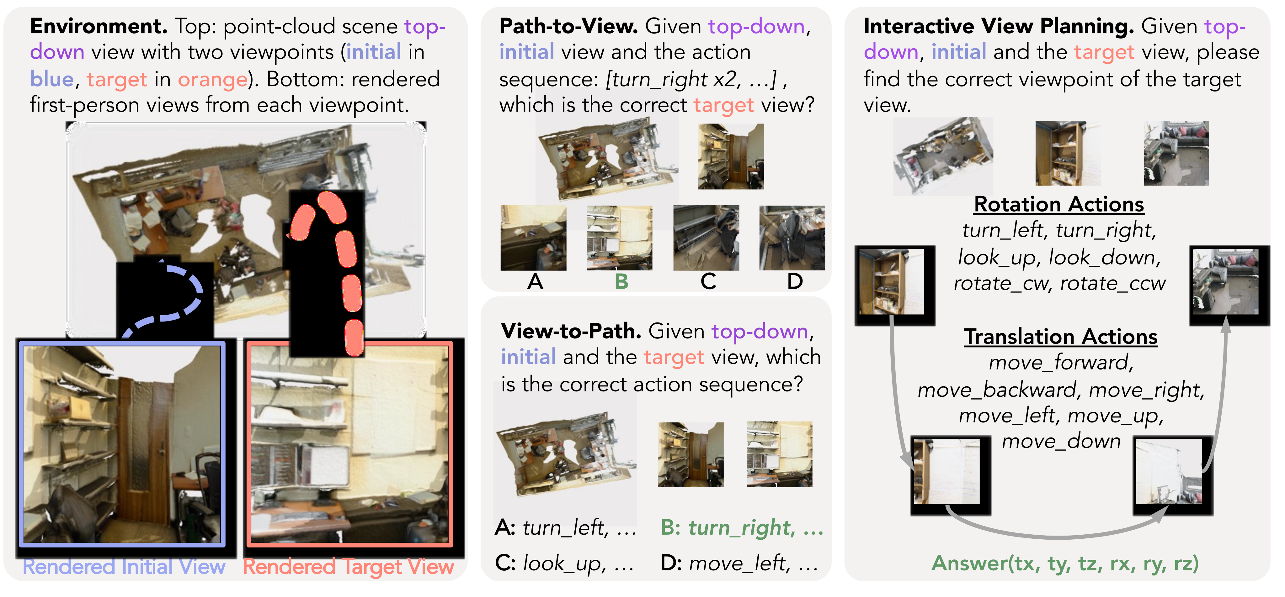
The environment makes camera actions, rendered observations and target poses measurable. Its three tasks share scene geometry while changing how much of the action sequence the model must construct.
2.1 Problem Formulation
A viewpoint consists of position and orientation. Initial and target images, a top-down reference and known action semantics define the task; the target camera pose remains to be inferred.
Path-to-View (P2V).
Path-to-View supplies the initial image and action sequence, then asks which of four candidate images is the resulting view. It measures forward tracking of the visual consequences of known actions.
View-to-Path (V2P).
View-to-Path supplies initial and target images, then asks which of four action sequences connects them. This tests selection among proposed transformations rather than free-form multi-step planning.
Interactive View Planning (IVP).
Interactive View Planning lets the model move the camera, observe the results and finally submit an estimated absolute target pose. The default budget is ten turns, including the answer. The main formulation judges that submitted estimate; physically reaching the target is not required.
2.2 Camera Pose Control Interface
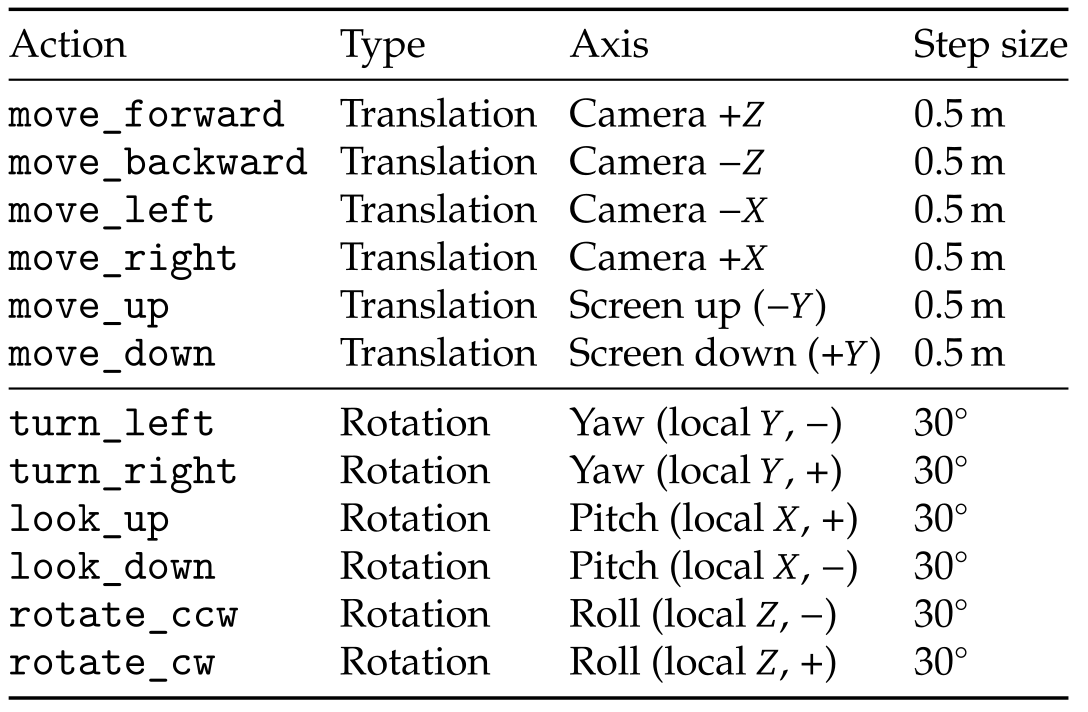
Twelve discrete actions translate along the three camera axes in either direction by 0.5 m, or rotate about them by 30°. Open3D renders new views from reconstructed point clouds. The interface exposes current pose and action/observation history, making this a controlled localization setting rather than uninstrumented robot navigation.
2.3 Data Collection and Evaluation
From 286 ScanNet scenes, the pipeline constructs roughly 55,000 viewpoint pairs and three tasks per pair, about 165,000 instances. Greedy camera-action planning, distractor perturbations and scene-quality filtering produce aligned examples. The reported experiments use the smaller ViewSuite-5K partition.
Dataset splits.
Scenes are split approximately 8:1:1 for training, validation and test. View pairs within each partition are divided about 1:10 into ViewSuite-5K and ViewSuite-50K. The test set used here has 530 pairs, or 1,590 task instances; the larger advertised collection is not the experiment count.
Evaluation metrics.
P2V/V2P use four-choice accuracy. IVP succeeds when the submitted pose has both position error at most 0.5 m and rotation error at most 30°, with rotation measured by the SO(3) geodesic in Equation 1. Appendix A calibrates these thresholds against human judgments. This conjunction differs from a single ball in the unified-distance metric.
Equation 1
| (1) |
Unified view distance.
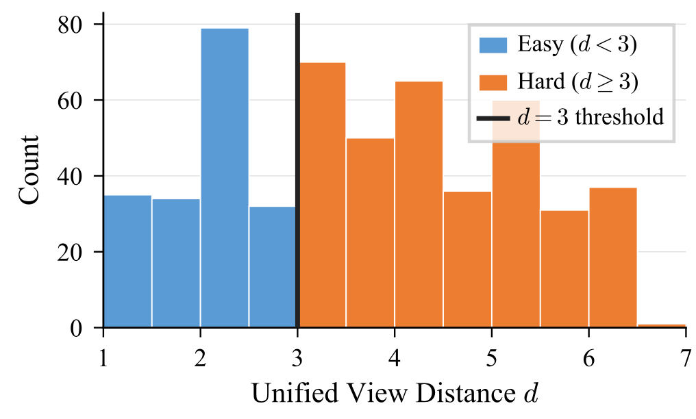
Equation 2 combines position error normalized by 0.5 m and orientation error normalized by 30° through a Euclidean norm. It is a dimensionless difficulty measure, not an exact minimum action count. Splitting at distance three yields 185 short and 345 long test pairs.
Equation 2
| (2) |
3 Planning Gap in Frontier VLMs
Thirteen models are evaluated on the same task family. The central comparison is the large gap between choosing among supplied single-turn alternatives and generating an effective multi-turn localization sequence.
3.1 Single-turn Tracking Understood, Multi-turn Planning Collapses
GPT-5.4 Pro leads P2V/V2P at 53.2/50.6%, but reaches only 19.9% IVP success; Gemini 3.1 Pro leads IVP at 21.3%. Qwen2.5-VL-7B starts at 2.5%, with no long-pair successes. Even the largest listed open model, Qwen3.5-397B, reaches only 4.3% IVP. GPT-5.4 Pro’s IVP denominator excludes 23 refusals: 101/507 gives 19.9%, whereas treating all 530 trials as attempts gives 19.1%.
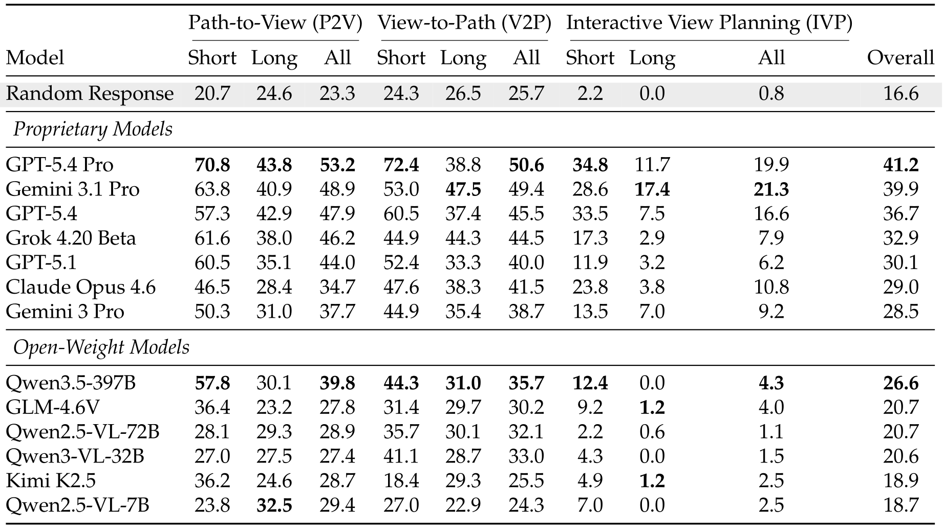
Original selectable table
| Path-to-View (P2V) | View-to-Path (V2P) | Interactive View Planning (IVP) | ||||||||
| Model | Short | Long | All | Short | Long | All | Short | Long | All | Overall |
| Random Response | 20.7 | 24.6 | 23.3 | 24.3 | 26.5 | 25.7 | 2.2 | 0.0 | 0.8 | 16.6 |
| Proprietary Models | ||||||||||
| GPT-5.4 Pro | 70.8 | 43.8 | 53.2 | 72.4 | 38.8 | 50.6 | 34.8 | 11.7 | 19.9 | 41.2 |
| Gemini 3.1 Pro | 63.8 | 40.9 | 48.9 | 53.0 | 47.5 | 49.4 | 28.6 | 17.4 | 21.3 | 39.9 |
| GPT-5.4 | 57.3 | 42.9 | 47.9 | 60.5 | 37.4 | 45.5 | 33.5 | 7.5 | 16.6 | 36.7 |
| Grok 4.20 Beta | 61.6 | 38.0 | 46.2 | 44.9 | 44.3 | 44.5 | 17.3 | 2.9 | 7.9 | 32.9 |
| GPT-5.1 | 60.5 | 35.1 | 44.0 | 52.4 | 33.3 | 40.0 | 11.9 | 3.2 | 6.2 | 30.1 |
| Claude Opus 4.6 | 46.5 | 28.4 | 34.7 | 47.6 | 38.3 | 41.5 | 23.8 | 3.8 | 10.8 | 29.0 |
| Gemini 3 Pro | 50.3 | 31.0 | 37.7 | 44.9 | 35.4 | 38.7 | 13.5 | 7.0 | 9.2 | 28.5 |
| Open-Weight Models | ||||||||||
| Qwen3.5-397B | 57.8 | 30.1 | 39.8 | 44.3 | 31.0 | 35.7 | 12.4 | 0.0 | 4.3 | 26.6 |
| GLM-4.6V | 36.4 | 23.2 | 27.8 | 31.4 | 29.7 | 30.2 | 9.2 | 1.2 | 4.0 | 20.7 |
| Qwen2.5-VL-72B | 28.1 | 29.3 | 28.9 | 35.7 | 30.1 | 32.1 | 2.2 | 0.6 | 1.1 | 20.7 |
| Qwen3-VL-32B | 27.0 | 27.5 | 27.4 | 41.1 | 28.7 | 33.0 | 4.3 | 0.0 | 1.5 | 20.6 |
| Kimi K2.5 | 36.2 | 24.6 | 28.7 | 18.4 | 29.3 | 25.5 | 4.9 | 1.2 | 2.5 | 18.9 |
| Qwen2.5-VL-7B | 23.8 | 32.5 | 29.4 | 27.0 | 22.9 | 24.3 | 7.0 | 0.0 | 2.5 | 18.7 |
3.2 What Bottlenecks Interactive View Planning?
Budget, renderer and difficulty analyses examine possible explanations for low IVP performance. They identify associations and sensitivity within the benchmark, without isolating every perceptual or reasoning mechanism.
Does turn budget affect IVP performance?
Raising the budget from ten to thirty turns changes IVP success from 21.3→23.2% for Gemini 3.1 Pro, 16.6→20.2 for GPT-5.4, 7.9→11.7 for Grok 4.20 Beta and 10.8→19.6 for Claude Opus 4.6. Extra interaction helps, particularly Claude, but leaves most tasks unsolved.
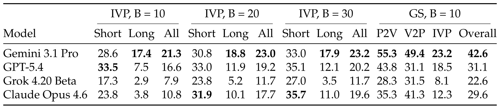
Original selectable table
| IVP, B = 10 | IVP, B = 20 | IVP, B = 30 | GS, B = 10 | ||||||||||
|---|---|---|---|---|---|---|---|---|---|---|---|---|---|
| Model | Short | Long | All | Short | Long | All | Short | Long | All | P2V | V2P | IVP | Overall |
| Gemini 3.1 Pro | 28.6 | 17.4 | 21.3 | 30.8 | 18.8 | 23.0 | 33.0 | 17.9 | 23.2 | 55.3 | 49.4 | 23.2 | 42.6 |
| GPT-5.4 | 33.5 | 7.5 | 16.6 | 33.0 | 11.9 | 19.2 | 35.1 | 12.1 | 20.2 | 43.8 | 31.1 | 18.5 | 31.1 |
| Grok 4.20 Beta | 17.3 | 2.9 | 7.9 | 23.8 | 5.2 | 11.7 | 27.0 | 3.5 | 11.7 | 28.3 | 31.5 | 8.1 | 22.6 |
| Claude Opus 4.6 | 23.8 | 3.8 | 10.8 | 31.9 | 10.1 | 17.7 | 35.7 | 11.0 | 19.6 | 35.3 | 41.3 | 12.3 | 29.6 |
Does rendering quality affect model performance?
Replacing point-cloud rendering with 3D Gaussian splatting changes the four tested models’ IVP scores by only 0.2–1.9 points at ten turns. Single-turn effects differ: Gemini’s P2V improves 6.4 points, while GPT-5.4 and Grok V2P decline 14.4 and 13.0. The experiment shows that this renderer substitution does not close the gap; it does not prove perception is irrelevant or isolate a purely cognitive bottleneck.
Is rotation or translation the primary difficulty driver?
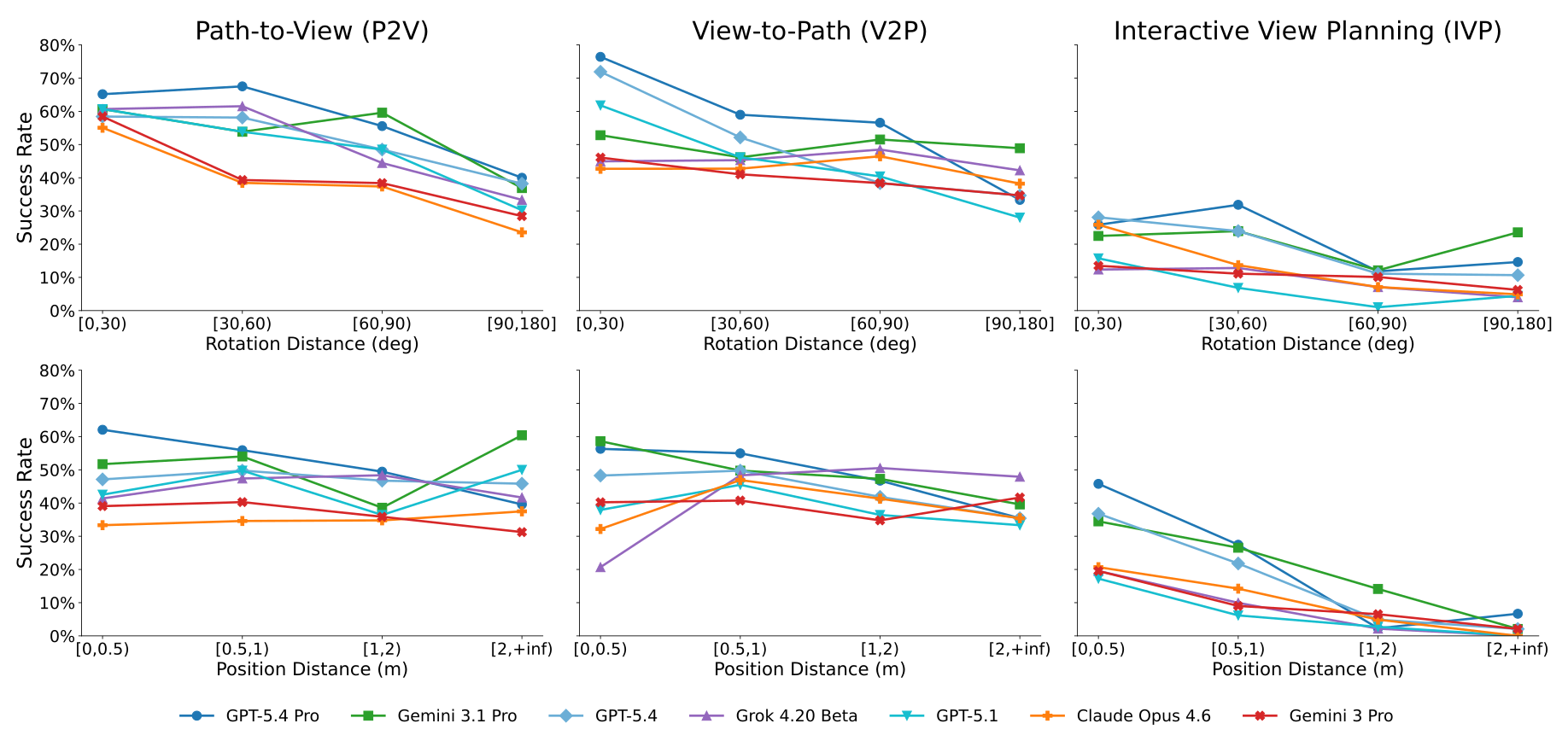
Figure 2 associates larger rotations with lower supplied-path tracking accuracy and larger translations with lower interactive success. The factor analysis similarly finds negative distance associations, with IVP position correlation as low as about −0.42. Correlations across geometrically different examples do not alone identify a causal failure mechanism.
Do successes reflect mental localization or view matching?
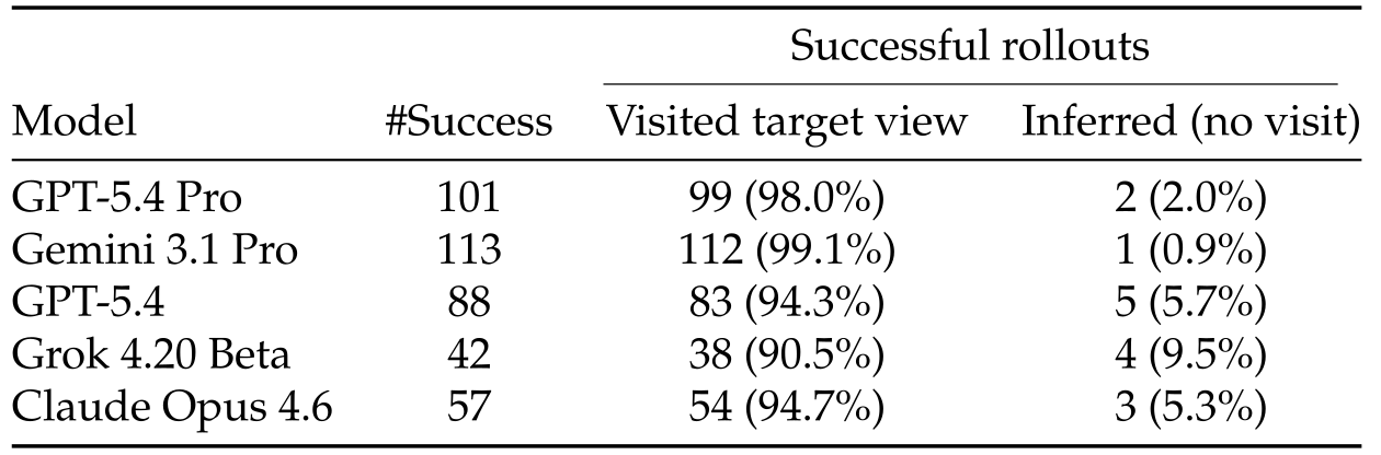
Among successful runs, 90–99% visit a pose within the target tolerance before submitting: 99/101 for GPT-5.4 Pro and 112/113 for Gemini. This is consistent with approaching and matching the target view. The visitation criterion is a geometric proxy, so it does not directly reveal the model’s internal reasoning or prove that every success lacks mental localization.
4 Self-Exploration with View Graph Distillation
The training loop converts experienced camera transitions into new tasks. A persistent graph connects viewpoints collected across episodes, allowing supervision from trajectories whose original goals were missed.
4.1 Interactive View Planning as a Localization Problem
IVP is framed as estimating the target camera pose from observations and known movements. A successful planner could infer that pose without standing there, so the desired capability goes beyond reaching a visually matching image. The study’s strongest empirical evidence is improved benchmark success, not a general guarantee of such inference.

4.2 Bootstrapping View Planning from Self-Exploration
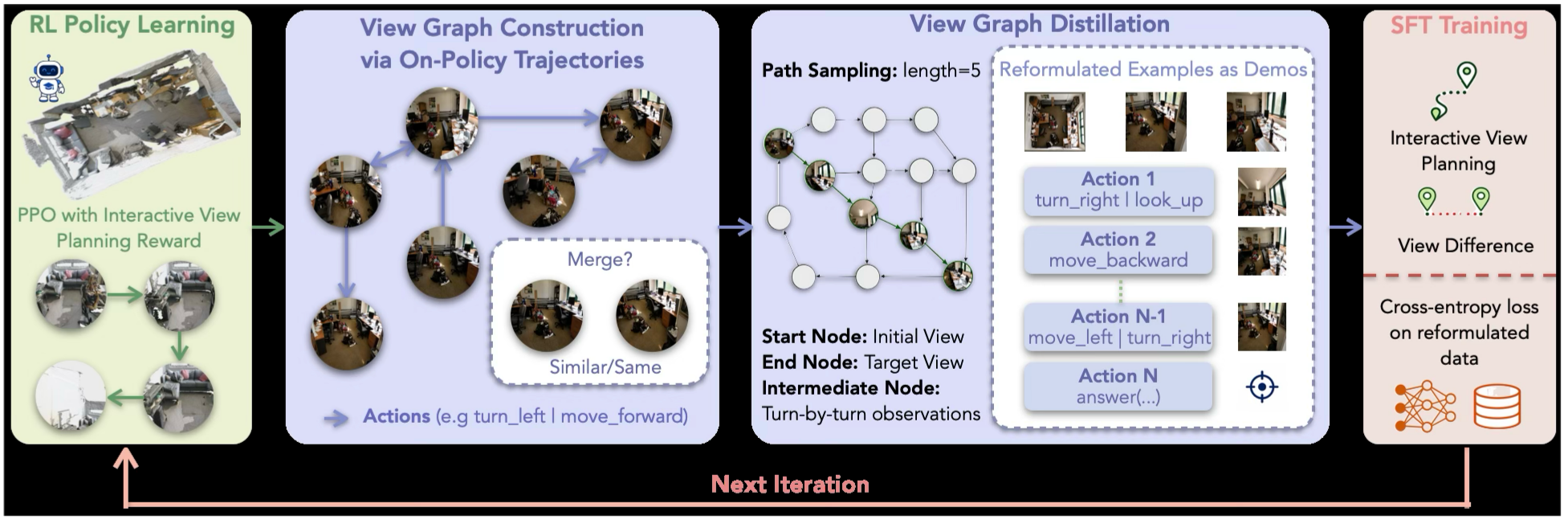
Alternate on-policy exploration and graph-derived supervised learning. The first three iterations use short RL phases followed by distillation; a final RL phase continues to convergence. New exploration enriches the same graph rather than replacing earlier experience.
Self-exploration stage.
PPO optimizes the reward in Equation 3: one for an accurate final target-pose estimate, plus 0.1 for valid output formatting. A background process records traversed poses, views and actions regardless of original task success. This provides useful transition data even when the sparse task reward remains zero.
View graph distillation via task reformulation.
For a sampled graph path, Equation 4 makes its first view the new initial observation and its final view/pose the new target, retaining the intervening actions as a demonstration. Auxiliary tasks estimate view distance directly or through multiple choice. This resembles hindsight relabeling, while the persistent graph can combine experience across episodes. Approximate node merging can change the start pose of redirected edges, so exact executability of every composed graph path is not guaranteed by the construction as described.
Equation 4
| (4) |
5 Self-Exploration Closes the Gap
The evaluation compares prompting, direct RL, successful-trajectory imitation and graph-distillation ablations. Its main result concerns held-out ViewSuite scenes and the specified camera interface.
5.1 Experimental Setup
The main backbone is Qwen2.5-VL-7B-Instruct; Qwen3-VL-8B tests a second starting model. All main IVP comparisons use the short/long split and default ten-turn protocol. Appendices provide training settings and relaxed-protocol results.
Prompting Baselines.
Prompted base Qwen2.5-VL-7B, GPT-5.4 Pro and Gemini 3.1 Pro serve as reference points. Their prior training, scale and inference mechanisms differ; the comparison is benchmark performance rather than a controlled architecture study.
Training Baselines.
Direct PPO uses the sparse task reward. A GRPO baseline filters rollout groups and trains for 1,000 steps. Success-only bootstrapping imitates completed original goals. These alternatives test whether reward optimization or filtering for success can replace learning from the broader transition graph.
Training Ablations.
Random-graph distillation removes policy-directed exploration. One- and two-iteration variants test how repeated graph expansion and supervised updates affect final RL performance. These comparisons assess complete recipes; the text does not establish equal graph diversity or total compute for every ablation.
5.2 Closing the Gap on Interactive View Planning
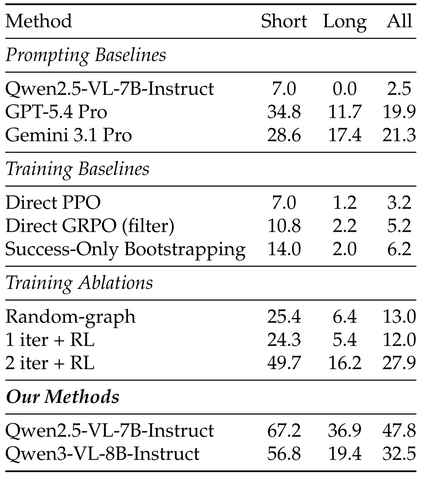
Full Qwen2.5 training reaches 47.8% overall, 67.2% short and 36.9% long, versus direct PPO 3.2%, filtered GRPO 5.2% and success-only bootstrapping 6.2%. Random graphs reach 13.0%; one and two iterations reach 12.0% and 27.9%. Qwen3-VL-8B reaches 32.5%. The gains support repeated graph distillation under these conditions, while more than half the main model’s test episodes remain unsolved.
Original selectable table
| Method | Short | Long | All |
|---|---|---|---|
| Prompting Baselines | |||
| Qwen2.5-VL-7B-Instruct | 7.0 | 0.0 | 2.5 |
| GPT-5.4 Pro | 34.8 | 11.7 | 19.9 |
| Gemini 3.1 Pro | 28.6 | 17.4 | 21.3 |
| Training Baselines | |||
| Direct PPO | 7.0 | 1.2 | 3.2 |
| Direct GRPO (filter) | 10.8 | 2.2 | 5.2 |
| Success-Only Bootstrapping | 14.0 | 2.0 | 6.2 |
| Training Ablations | |||
| Random-graph | 25.4 | 6.4 | 13.0 |
| 1 iter + RL | 24.3 | 5.4 | 12.0 |
| 2 iter + RL | 49.7 | 16.2 | 27.9 |
| Our Methods | |||
| Qwen2.5-VL-7B-Instruct | 67.2 | 36.9 | 47.8 |
| Qwen3-VL-8B-Instruct | 56.8 | 19.4 | 32.5 |
5.3 What Has the Model Learned?
Coverage, attention and downstream adaptation probe what changes with training. They offer complementary behavioral and representational evidence, with different limits on causal interpretation.
What exploration strategy does the trained model learn?
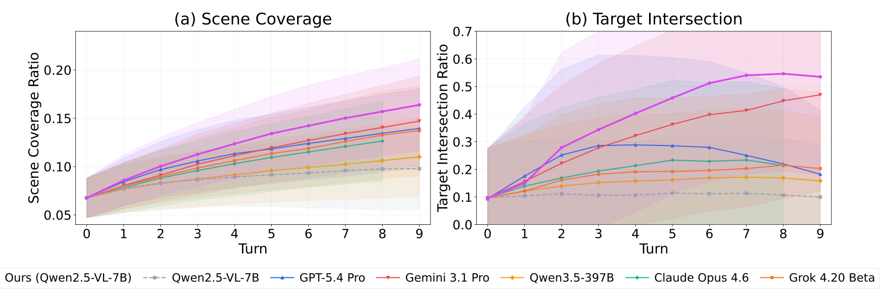
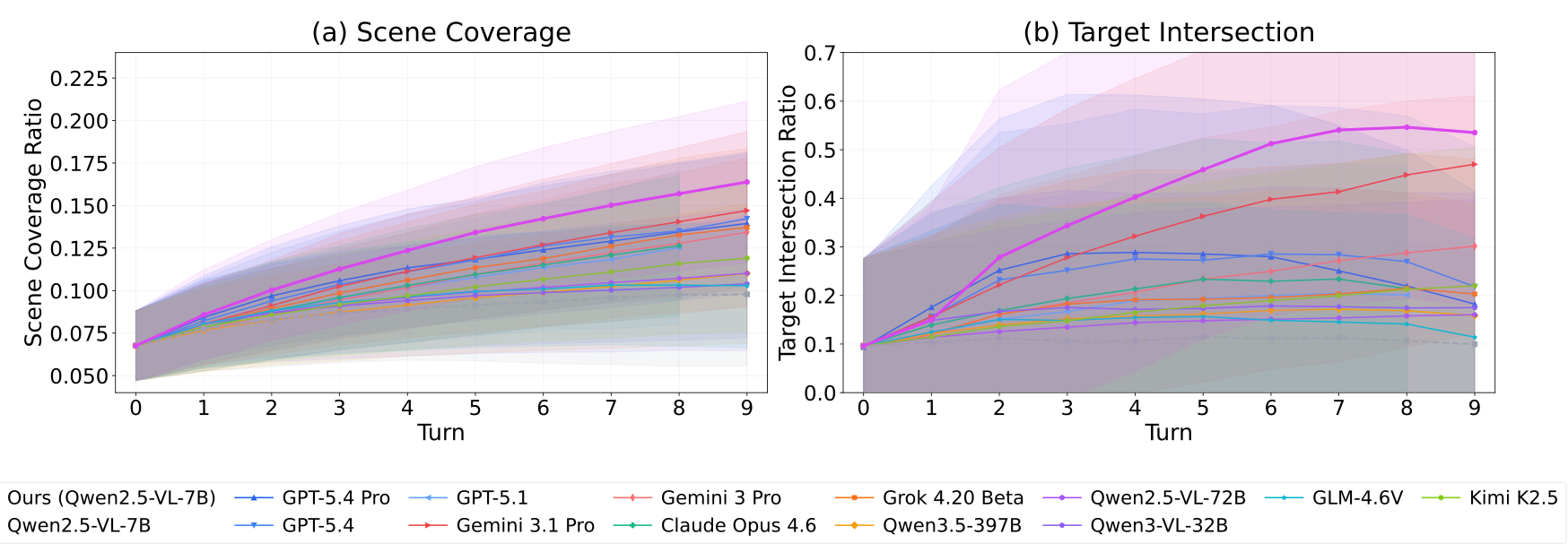
The trained model’s aggregate coverage grows toward about 55% of target-visible vertices, exceeding the comparison models. The authors interpret this as exploration followed by target-directed approach. Because coverage uses a cumulative union, it cannot decrease within a fixed trajectory; declines in per-turn averages can instead reflect early stopping and changes in which rollouts remain. The trained curve also dips slightly at its final point, so strict monotonicity is not established.
How does training reshape the model’s attention?
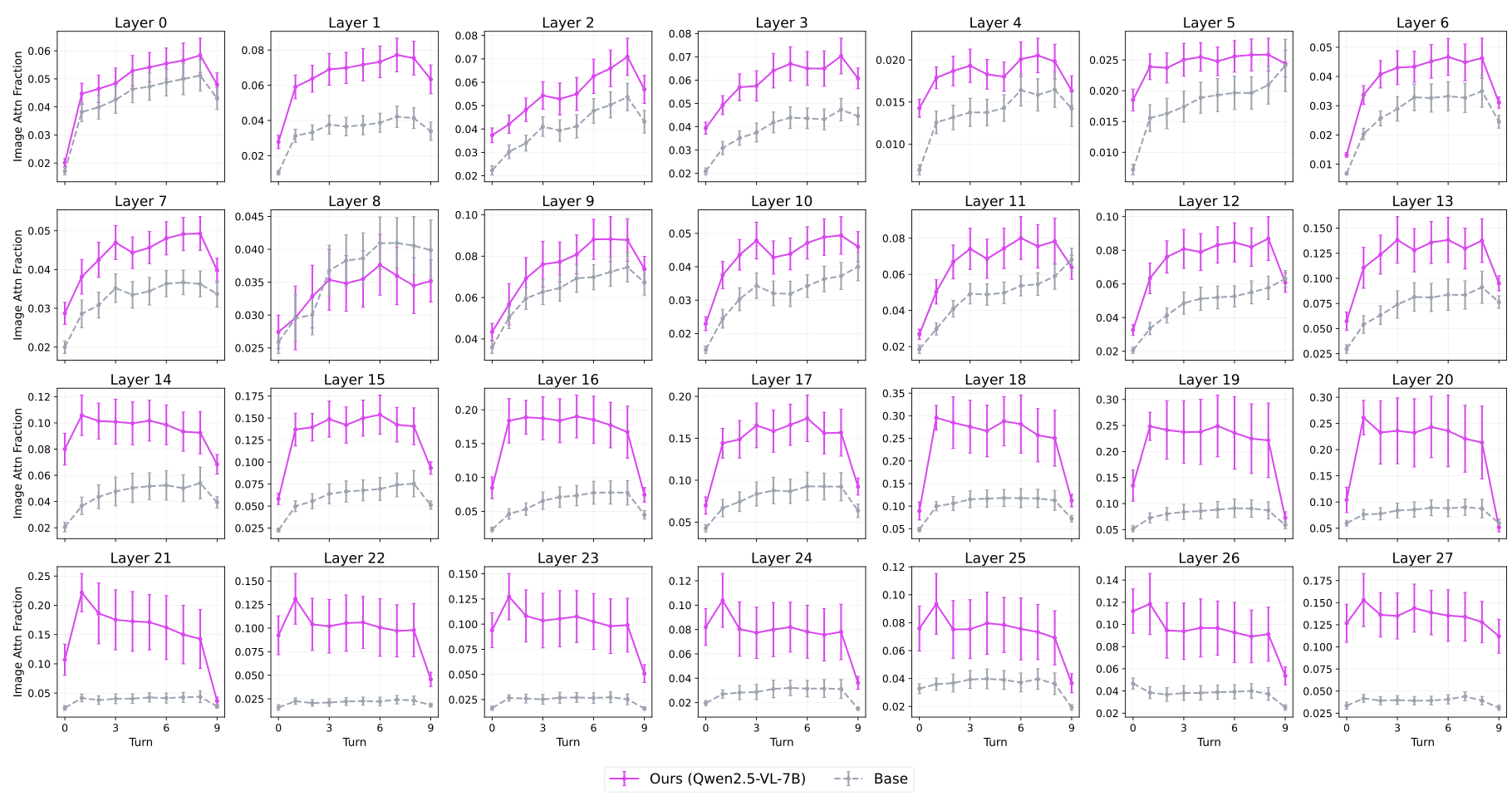
On the same trajectories, the trained model gives image tokens more response-token attention across nearly all 28 layers. Mean trained/base ratios are 1.4× in layers 0–8, 1.9× in 9–18 and 3.0× in 19–27. Increased attention is consistent with stronger visual use, but attention fractions alone do not establish causality or an internal 3D world model.
Do the learned priors transfer to other view-related tasks?
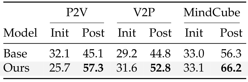
After additional matched GRPO training, the view-trained initialization beats the base by 12.2 points on P2V (57.3 vs 45.1), 8.0 on V2P (52.8 vs 44.8) and 9.9 on MindCube (66.2 vs 56.3). These are adaptation gains, not zero-shot transfer. Initial P2V is actually lower for the trained model, 25.7 vs 32.1. Table 6’s base initial P2V/V2P scores differ from Table 2’s 29.4/24.3, without an explicit reconciliation.
6 Related Work
View reasoning and 3D scene benchmarks.
MindCube, ViewSpatial-Bench, CameraBench and multi-image spatial evaluations test viewpoint relationships; ScanQA and SQA3D emphasize scene questions. ViewSuite adds controllable multi-turn viewpoint acquisition. The links to cognitive maps and mental rotation motivate the task but do not themselves validate a model’s cognitive mechanism.
Visual search and active perception.
Active perception and active vision choose observations to reduce uncertainty. Recent V*, ActiView and embodied search work control crops or viewpoints. This paper emphasizes six-degree-of-freedom camera actions and pose localization in reconstructed scenes, distinct from unrestricted physical navigation.
Agentic RL and learning from failure.
STaR, self-imitation, on-policy distillation and hindsight trajectory rewriting turn model experience into training data. Here the graph’s observed geometric transitions supply demonstrations even when the original episode fails; it therefore avoids depending solely on rare initial successes or a stronger teacher.
7 Conclusion and Limitations
Accumulating and reformulating experienced transitions supplies a useful learning signal where direct sparse-reward training struggles. The results establish substantial gains on ViewSuite and improved downstream adaptation, while leaving the interpretation of unseen-view reasoning and broader generalization open.
Limitations.
Evaluation uses static indoor reconstructions, discrete camera actions and 7B/8B backbones. Outdoor scenes, dynamic objects, continuous controls and much larger models are untested. The trained agent still often approaches until it sees the target; explicit reasoning traces and localization without such matching remain unresolved.
Acknowledgements
The authors disclose AI-tool use in coding and paper writing, and thank Jiajun Liu, Baiqiao Yin, Jiawei Gu and Jihan Yang for discussions.
Appendix
Appendix A ViewSuite Details
A.1 Action Space Details
The camera follows OpenCV axes: +X right, +Y down and +Z forward; the ScanNet world frame is Z-up. Table 7 retains all twelve signed local-axis actions.
Translation actions.
Forward/backward translate ±Z, right/left ±X, and down/up ±Y in the current camera frame, each by 0.5 m. These are camera-relative moves rather than fixed world-axis offsets.
Rotation actions.
Left/right turns rotate about local Y, look up/down about local X, and counter-clockwise/clockwise rolls about local Z. Each signed step is 30° and rotates about the camera center.
Discrete snapping.
After each rotation, the described procedure decomposes the camera-to-world matrix into intrinsic XYZ Euler angles, rounds each to 30° and recomposes it. This enforces an Euler grid but does not generally make local-axis actions exactly invertible. For example, starting at (−60,−60,−30)°, a local Y +30° move and its −30° inverse, each followed by this snapping, end at (−60,−60,−60)°, 30° from the start. This checks the stated mathematical procedure, not uninspected implementation behavior.
Original selectable table
| Action | Type | Axis | Step size |
|---|---|---|---|
| move_forward | Translation | Camera | m |
| move_backward | Translation | Camera | m |
| move_left | Translation | Camera | m |
| move_right | Translation | Camera | m |
| move_up | Translation | Screen up () | m |
| move_down | Translation | Screen down () | m |
| turn_left | Rotation | Yaw (local , ) | |
| turn_right | Rotation | Yaw (local , ) | |
| look_up | Rotation | Pitch (local , ) | |
| look_down | Rotation | Pitch (local , ) | |
| rotate_ccw | Rotation | Roll (local , ) | |
| rotate_cw | Rotation | Roll (local , ) |
A.2 Data Sampling and Filtering Pipeline
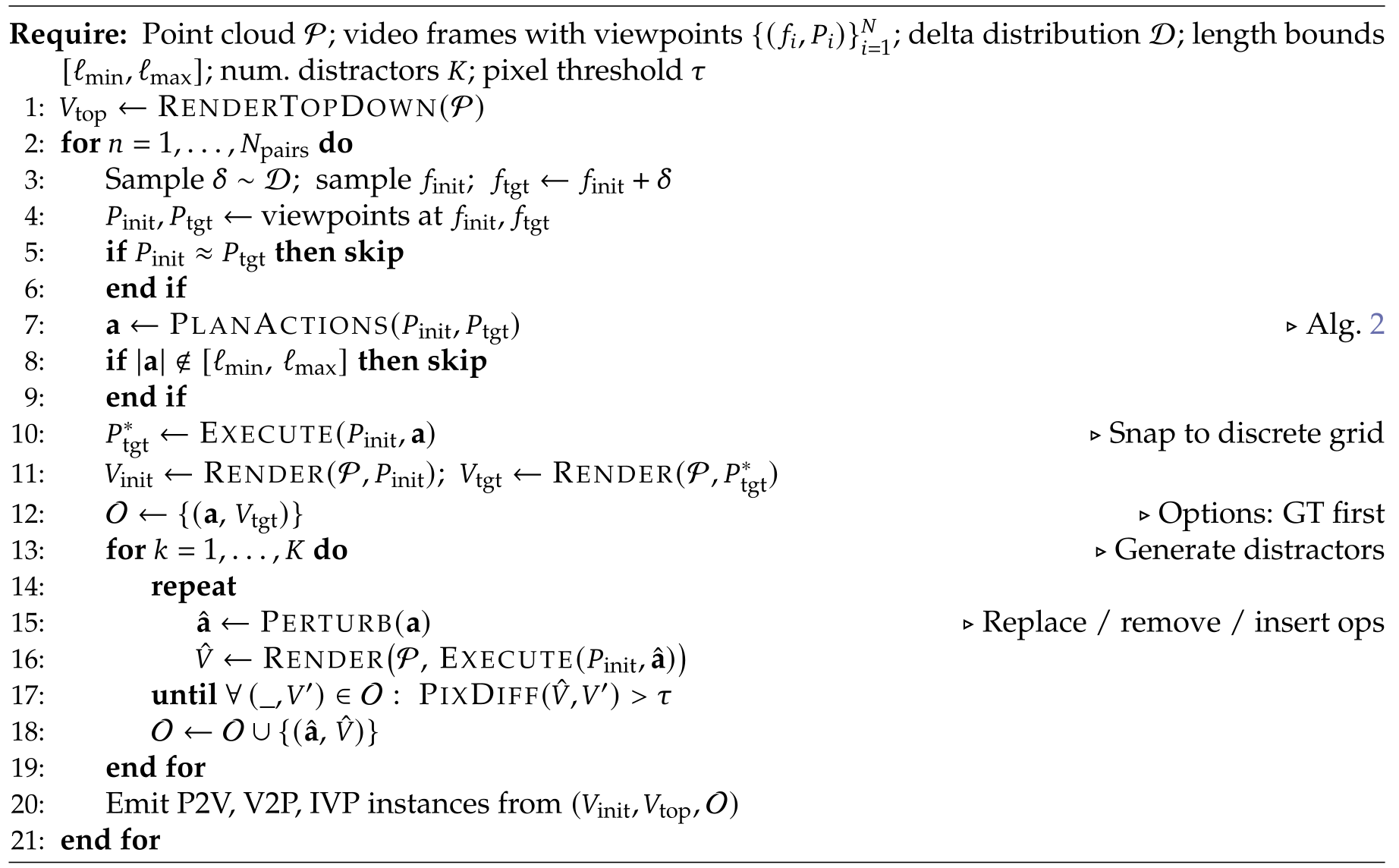
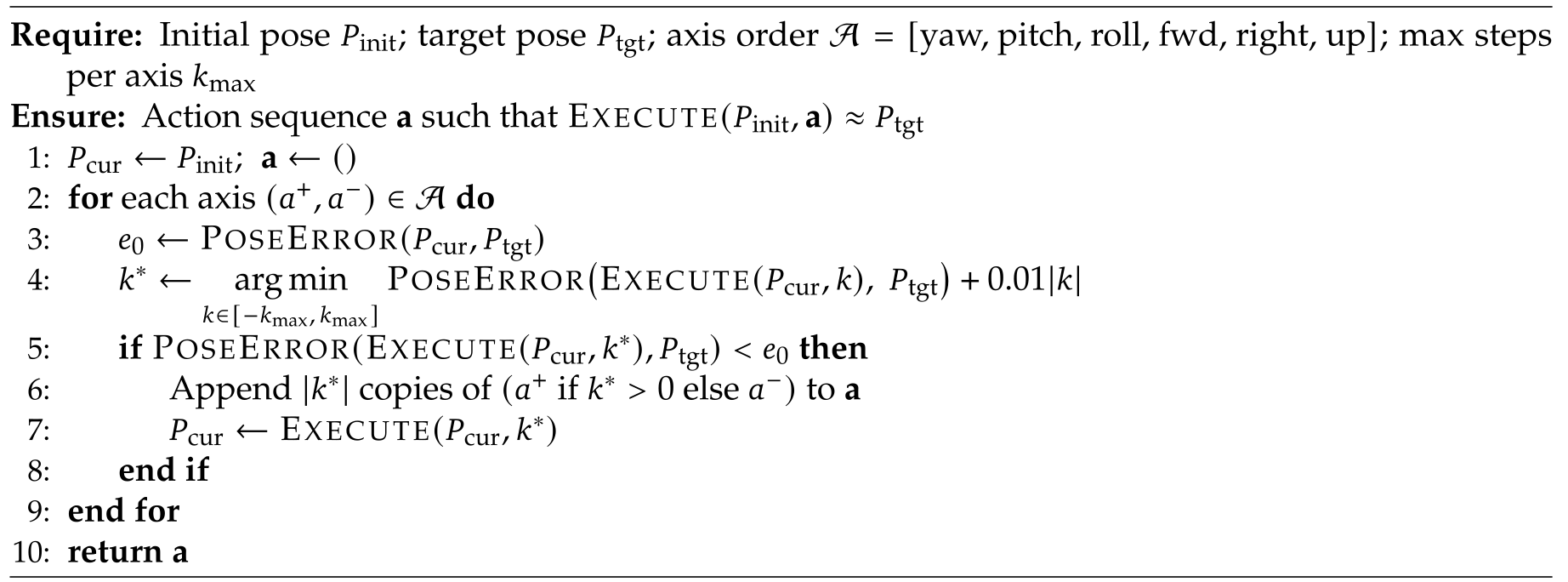
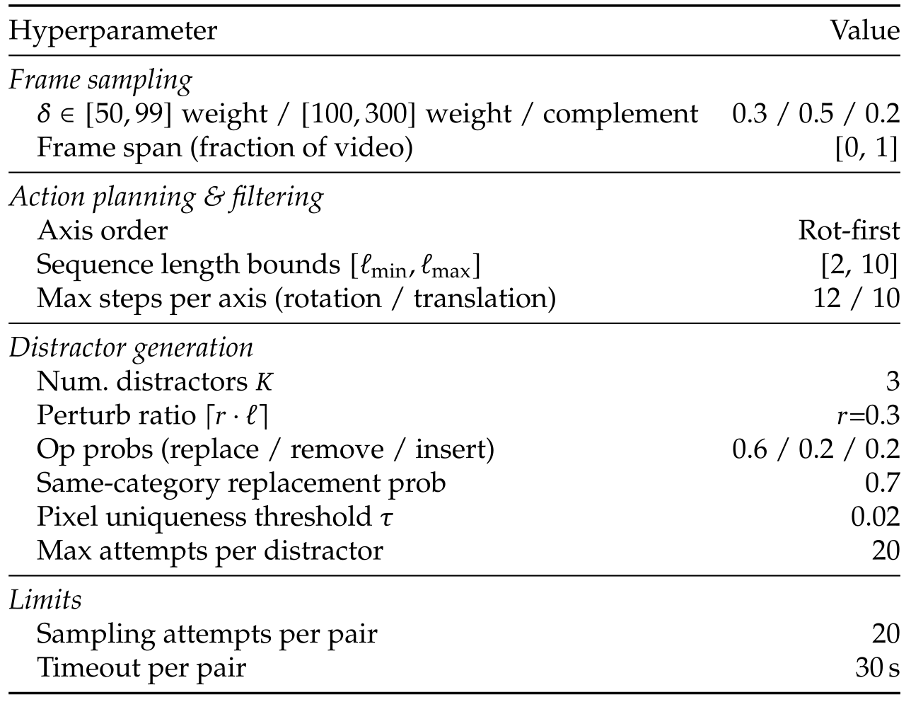
Algorithms 1–2 and Table 8 preserve the construction pipeline: select frame pairs, find a short discrete path, create distractors and reject unsuitable views/scenes. The pipeline uses known reconstructed geometry and poses.
Frame sampling.
Temporal gaps are sampled from 50–99 frames with weight 0.3, 100–300 with 0.5, and remaining valid indices with 0.2. This favors substantial viewpoint changes while retaining nearby examples.
Action planning.
A deterministic greedy planner processes yaw, pitch, roll, forward, right and up in that order. It searches signed step counts on each axis, favors lower pose error with a small length penalty, and retains sequences of two to ten actions. This is a heuristic construction procedure, not a globally optimal path solver.
Distractor generation.
Three distractors perturb about 30% of the true sequence by replacement, removal or insertion with probabilities 0.6/0.2/0.2. Replacement favors the same motion category with probability 0.7. Rendered options must differ by at least 0.02 mean pixel difference; attempt/time limits are preserved in Table 8.
Scene-level filtering.
A VLM judges top-down scene views using twelve examples, six usable and six obscured, followed by manual verification. Scenes with poor visible layout are removed. Thus teacher-free policy training does not mean the entire dataset was assembled without model-assisted filtering or human checks.
Original selectable algorithm
Original selectable algorithm
Original selectable table
| Hyperparameter | Value |
| Frame sampling | |
| weight / weight / complement | 0.3 / 0.5 / 0.2 |
| Frame span (fraction of video) | |
| Action planning & filtering | |
| Axis order | Rot-first |
| Sequence length bounds | |
| Max steps per axis (rotation / translation) | 12 / 10 |
| Distractor generation | |
| Num. distractors | 3 |
| Perturb ratio | |
| Op probs (replace / remove / insert) | 0.6 / 0.2 / 0.2 |
| Same-category replacement prob | 0.7 |
| Pixel uniqueness threshold | 0.02 |
| Max attempts per distractor | 20 |
| Limits | |
| Sampling attempts per pair | 20 |
| Timeout per pair | 30 s |
A.3 Success Threshold Calibration
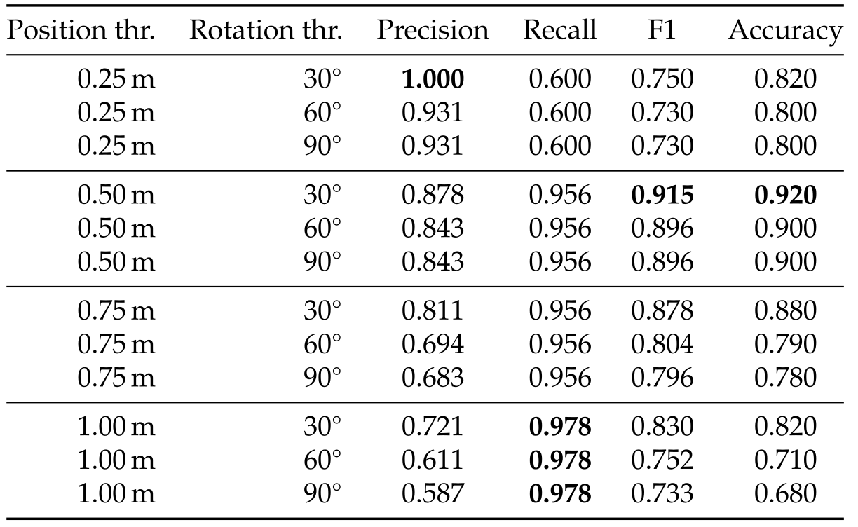
Experts compare submitted and target renders, then twelve pose-threshold combinations are evaluated against their match judgments. The chosen 0.5 m/30° pair has precision 0.878, recall 0.956, F1 0.915 and accuracy 0.920. Larger tolerances increase recall but reduce precision. The study does not report the number of judged examples, annotators or inter-annotator agreement.
Original selectable table
| Position thr. | Rotation thr. | Precision | Recall | F1 | Accuracy |
|---|---|---|---|---|---|
| m | 1.000 | 0.600 | 0.750 | 0.820 | |
| m | 0.931 | 0.600 | 0.730 | 0.800 | |
| m | 0.931 | 0.600 | 0.730 | 0.800 | |
| m | 0.878 | 0.956 | 0.915 | 0.920 | |
| m | 0.843 | 0.956 | 0.896 | 0.900 | |
| m | 0.843 | 0.956 | 0.896 | 0.900 | |
| m | 0.811 | 0.956 | 0.878 | 0.880 | |
| m | 0.694 | 0.956 | 0.804 | 0.790 | |
| m | 0.683 | 0.956 | 0.796 | 0.780 | |
| m | 0.721 | 0.978 | 0.830 | 0.820 | |
| m | 0.611 | 0.978 | 0.752 | 0.710 | |
| m | 0.587 | 0.978 | 0.733 | 0.680 |
A.4 View Distance Distribution
Across 530 test pairs, unified distance ranges about 1.4–6.8 with mean 3.7. The threshold at three separates 185 short from 345 long cases. Its interpretation as roughly three micro-actions is a heuristic, since the combined norm is not the discrete planner’s exact path length.
A.5 Task Examples
The original prompt examples and their figures are retained below, including all image placeholders and answer formats. The IVP prompt is already abridged in the paper, which omits its full action list.
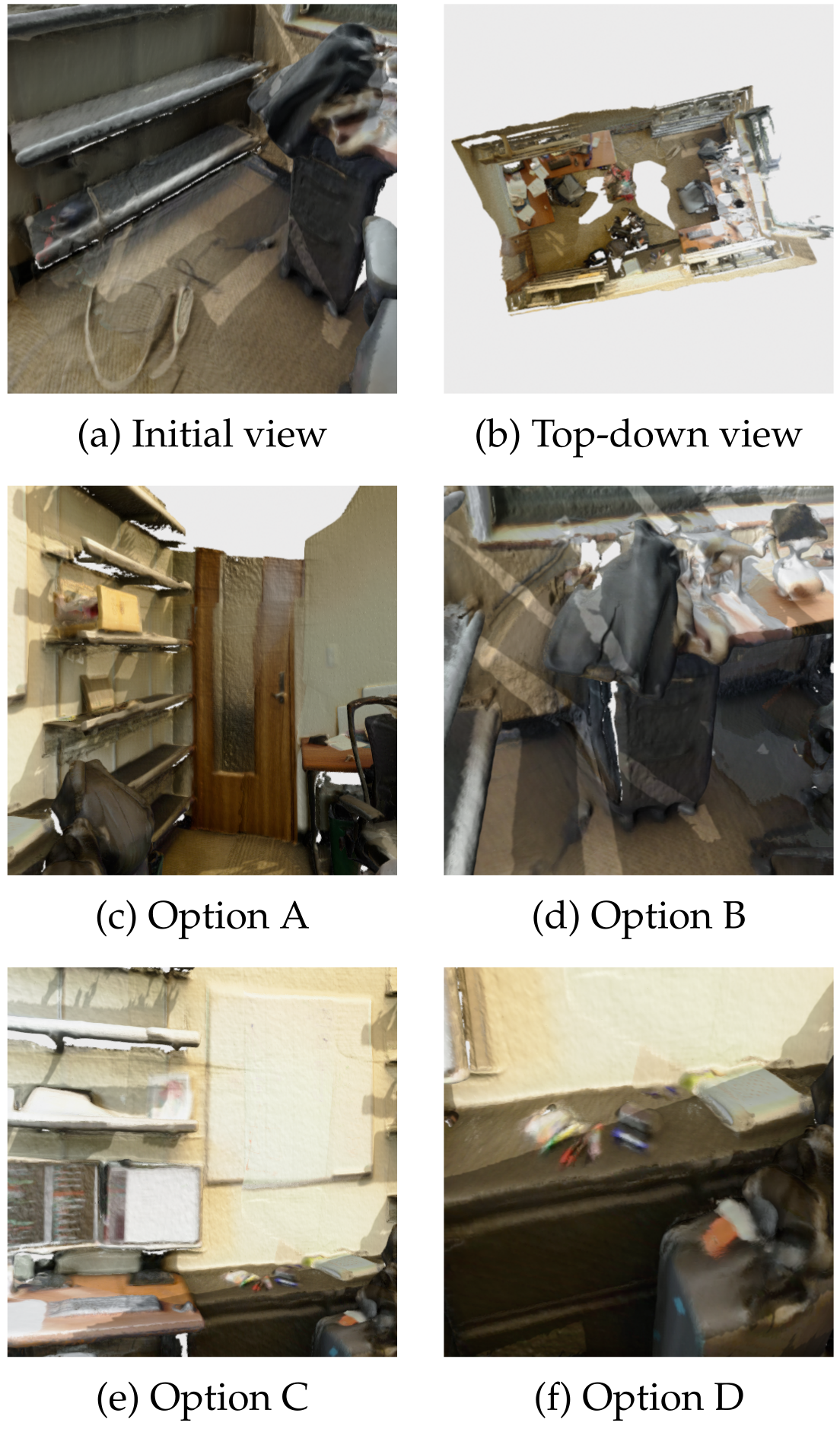
Path-to-View (P2V).
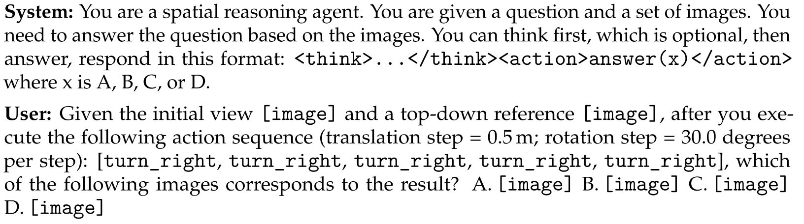
Figure 7 applies five right turns and asks for the resulting image. GPT-5.4 Pro chooses C incorrectly. This is an illustrative failure, not a frequency estimate.
Original selectable text and notation
System: You are a spatial reasoning agent. You are given a question and a set of images. You need to answer the question based on the images. You can think first, which is optional, then answer, respond in this format: <think>...</think><action>answer(x)</action> where x is A, B, C, or D.
User: Given the initial view [image] and a top-down reference [image], after you execute the following action sequence (translation step = 0.5 m; rotation step = 30.0 degrees per step): [turn_right, turn_right, turn_right, turn_right, turn_right], which of the following images corresponds to the result? A. [image] B. [image] C. [image] D. [image]
View-to-Path (V2P).
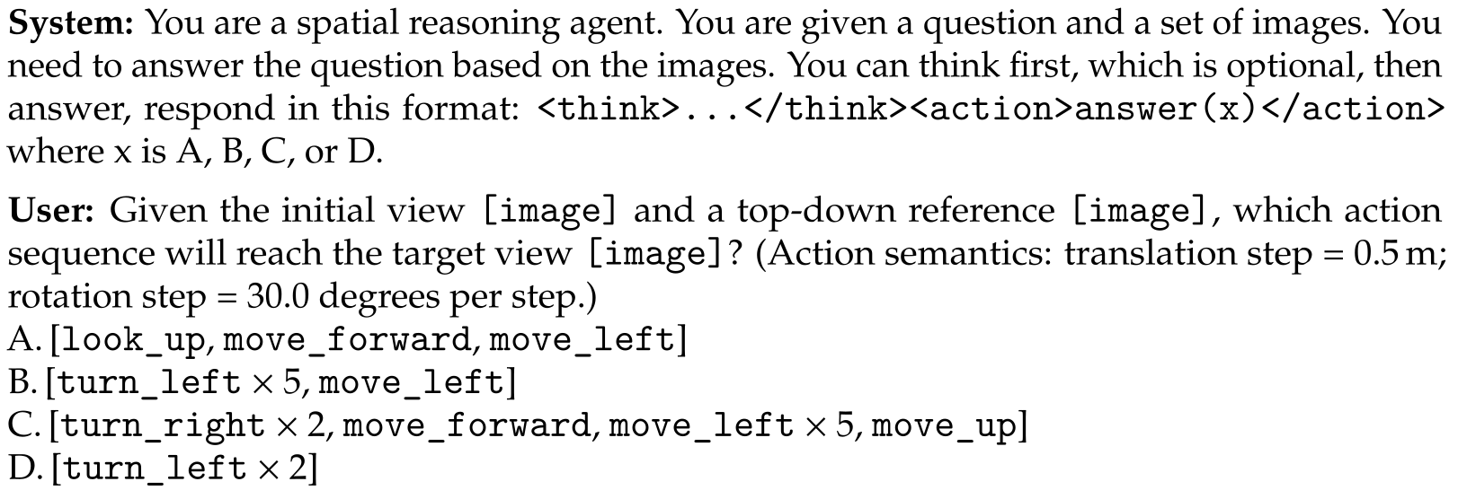
Figure 8 asks which sequence reaches the target. GPT-5.4 Pro correctly chooses B: five left turns followed by a left translation. The retained prompt contains all four alternatives.
Original selectable text and notation
System: You are a spatial reasoning agent. You are given a question and a set of images. You need to answer the question based on the images. You can think first, which is optional, then answer, respond in this format: <think>...</think><action>answer(x)</action> where x is A, B, C, or D.
User: Given the initial view [image] and a top-down reference [image], which action sequence will reach the target view [image]? (Action semantics: translation step = 0.5 m; rotation step = 30.0 degrees per step.)
A. [look_up, move_forward, move_left]
B. [turn_left 5, move_left]
C. [turn_right 2, move_forward, move_left 5, move_up]
D. [turn_left 2]
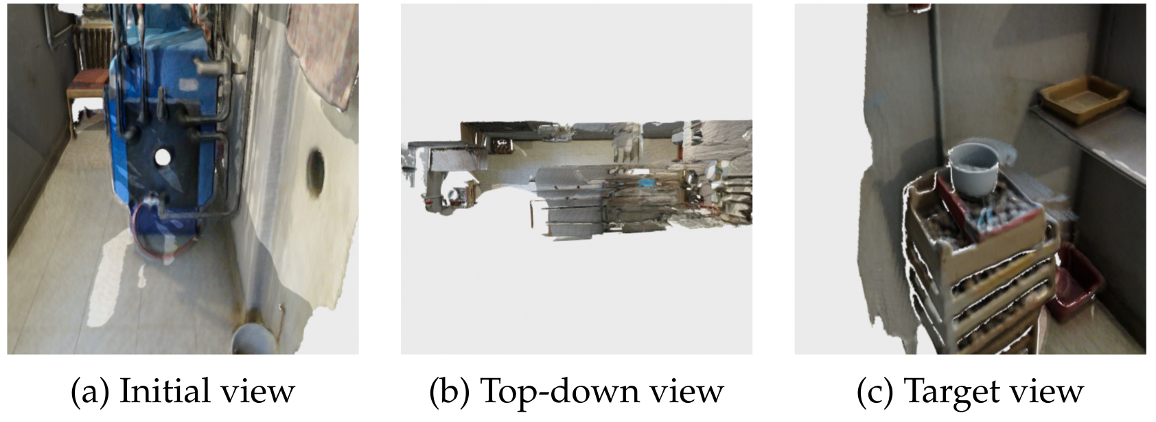
Interactive View Planning (IVP).
In Figure 9, the trained model uses right turns, a downward look, a left translation and a forward move before answering on turn six. Its final estimate has 0.061 m position error and 0° rotation error. The prompt explicitly requests an absolute target-pose estimate and separate position/rotation thresholds.
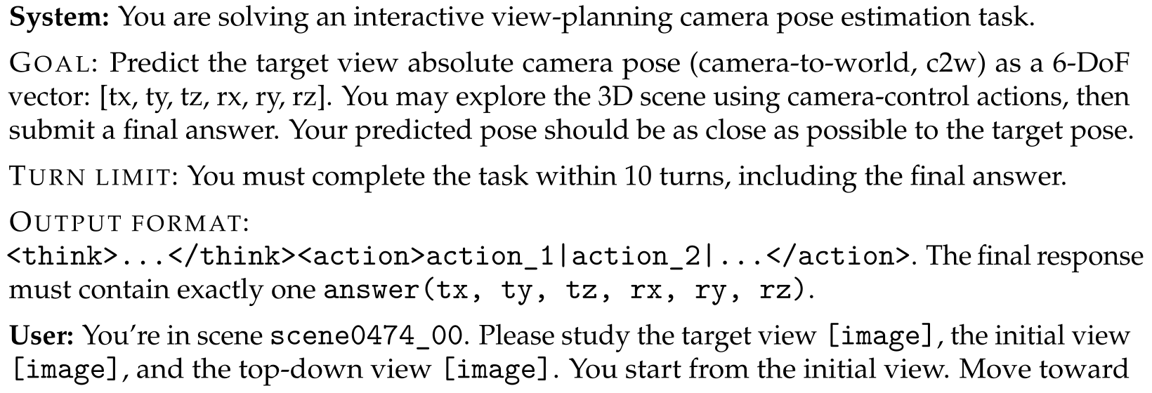

Original selectable text and notation
System: You are solving an interactive view-planning camera pose estimation task.
Goal: Predict the target view absolute camera pose (camera-to-world, c2w) as a 6-DoF vector: [tx, ty, tz, rx, ry, rz]. You may explore the 3D scene using camera-control actions, then submit a final answer. Your predicted pose should be as close as possible to the target pose.
Turn limit: You must complete the task within 10 turns, including the final answer.
Output format:
<think>...</think><action>action_1|action_2|...</action>. The final response must contain exactly one answer(tx, ty, tz, rx, ry, rz).User: You’re in scene scene0474_00. Please study the target view [image], the initial view [image], and the top-down view [image]. You start from the initial view. Move toward the target view using actions. Initial view camera 6-DoF: [tx=4.07, ty=3.28, tz=1.66, rx=, ry=, rz=]. Success thresholds: position error 0.5 m, rotation error .
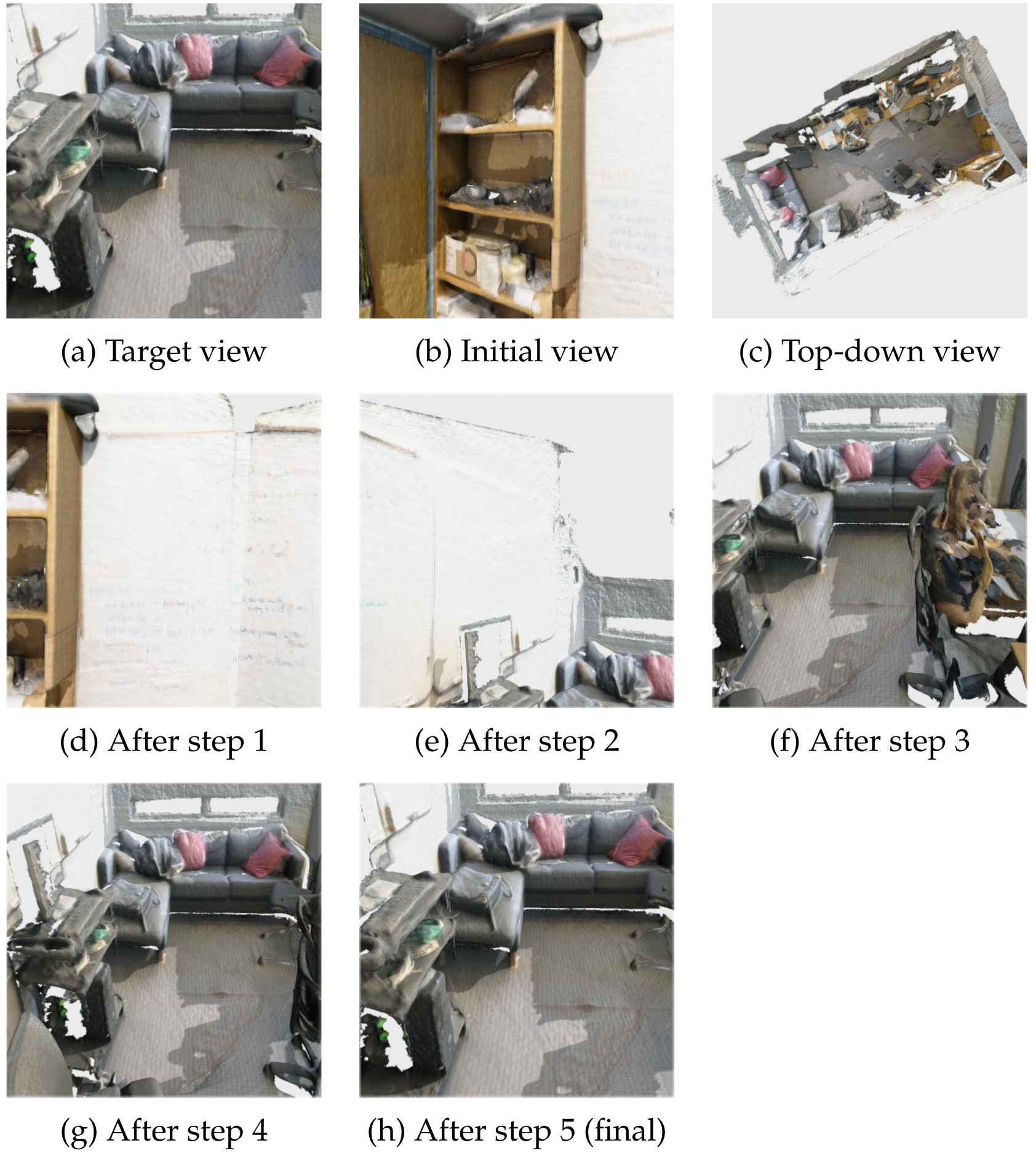
Appendix B Extended Evaluation Results
B.1 Evaluation-Protocol Ablations on IVP
Removing snapping lowers trained Qwen2.5 success from 47.8 to 19.6%; counting any target encounter without a final submission raises it to 60.2%. Trained Qwen3 obtains 18.5 and 48.3%; Gemini obtains 15.7 and 31.5. The model ordering survives, but absolute performance depends strongly on the protocol.
Appendix B describes default success as the current pose being within a unified-distance threshold when submitting. That differs from the main text/prompt’s submitted target estimate and separate position/rotation bounds. No-Submit also changes localization into an encounter criterion. These descriptions should not be silently treated as equivalent.
Coverage note for GPT-5.4 Pro.
GPT-5.4 Pro refuses 23 of 530 IVP examples and is scored over its remaining 507 valid episodes, yielding 101/507 = 19.9%. Other listed models use all 530. Its P2V and V2P evaluations also use all 530 pairs.
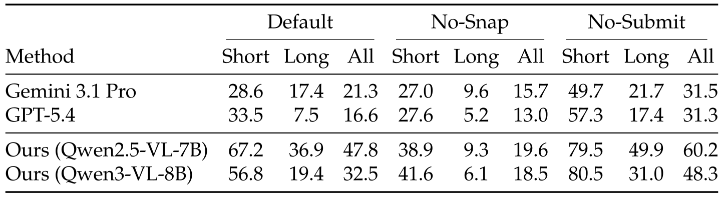
Original selectable table
| Default | No-Snap | No-Submit | |||||||
|---|---|---|---|---|---|---|---|---|---|
| Method | Short | Long | All | Short | Long | All | Short | Long | All |
| Gemini 3.1 Pro | 28.6 | 17.4 | 21.3 | 27.0 | 9.6 | 15.7 | 49.7 | 21.7 | 31.5 |
| GPT-5.4 | 33.5 | 7.5 | 16.6 | 27.6 | 5.2 | 13.0 | 57.3 | 17.4 | 31.3 |
| Ours (Qwen2.5-VL-7B) | 67.2 | 36.9 | 47.8 | 38.9 | 9.3 | 19.6 | 79.5 | 49.9 | 60.2 |
| Ours (Qwen3-VL-8B) | 56.8 | 19.4 | 32.5 | 41.6 | 6.1 | 18.5 | 80.5 | 31.0 | 48.3 |
B.2 Sample-Level Factor Analysis
Spearman correlations link twelve geometric/visibility factors with binary task success. Same-facing orientation correlates positively with P2V/V2P, approximately +0.19 to +0.30, while position distance is the strongest negative IVP factor. Grok’s weak or positive V2P distance association is an outlier, not evidence by itself of a specific reasoning strategy. Figure 10 displays models as rows and factors as columns, reversing the caption’s verbal row/column description.
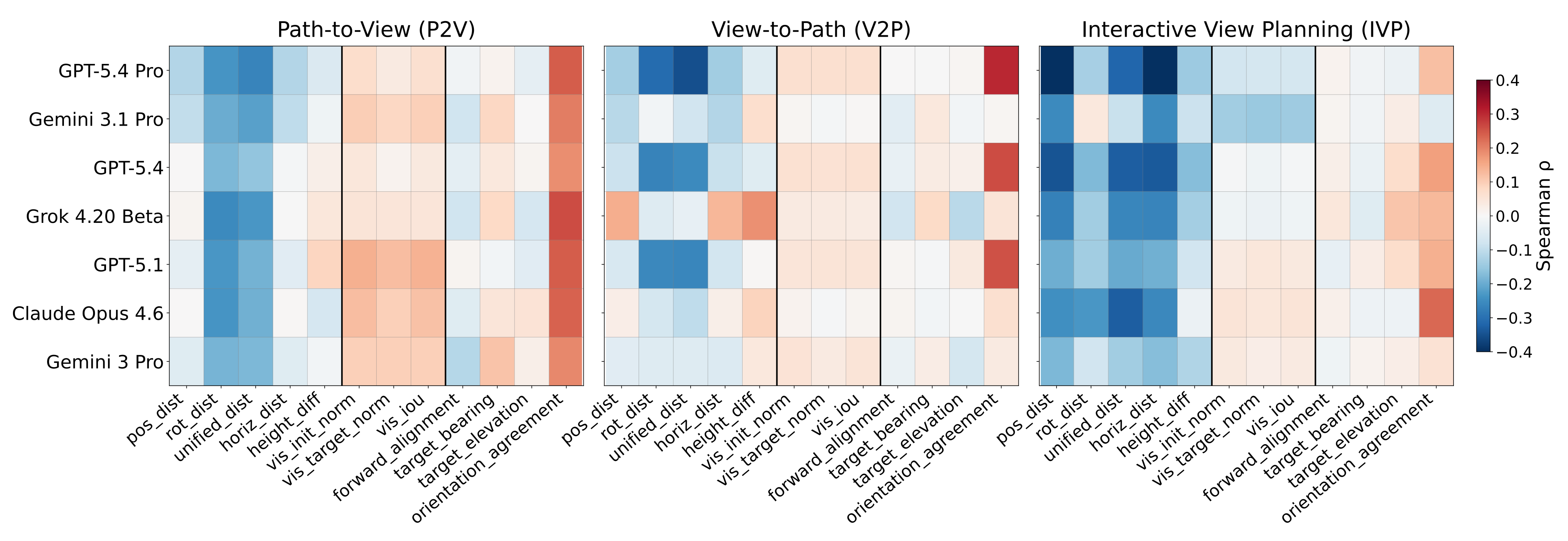
B.3 Success Factor Definitions
The exact factor definitions are retained with their notation. One convention is inconsistent: this subsection defines camera forward as −R[:,2], whereas Appendix A uses OpenCV +Z forward. A common sign flip leaves pairwise orientation agreement unchanged but changes target-bearing and forward-alignment signs; the paper does not explain a frame conversion.

Original selectable text and notation
We define the sample-level factors used in Figure 10. All factors are computed from the initial and target camera-to-world extrinsics ( matrices) shared across the test view pairs. We write position (the translation column), rotation (the rotation submatrix), and camera forward direction (negative z-axis of the camera frame, transformed to world coordinates).
Group A: Geometric Distance.
The five distance factors are Euclidean position, SO(3) rotation, normalized combined distance, horizontal displacement and absolute height difference. Their original formulas and units are retained below.


Original selectable text and notation
- •
pos_dist (): (meters). Euclidean distance between camera positions.
- •
rot_dist (): (degrees). Geodesic angle between orientations.
- •
unified_dist: (steps), where m and are the discrete step sizes in ViewSuite. Equivalent to the unified view distance defined in Section 2.
- •
horiz_dist: (meters). Horizontal distance, ignoring vertical displacement.
- •
height_diff: (meters). Absolute vertical difference.
Group B: Visual Overlap.
Depth-rendered visible vertex sets define overlap normalized by the initial set, overlap normalized by the target set, and intersection-over-union. These quantities distinguish how much of each view is shared.
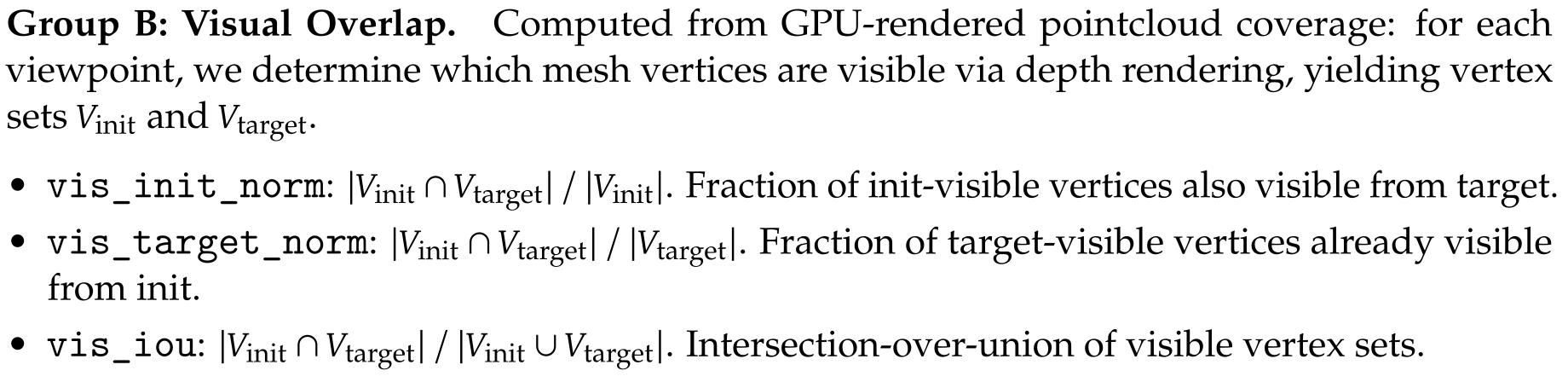
Original selectable text and notation
Computed from GPU-rendered pointcloud coverage: for each viewpoint, we determine which mesh vertices are visible via depth rendering, yielding vertex sets and .
- •
vis_init_norm: . Fraction of init-visible vertices also visible from target.
- •
vis_target_norm: . Fraction of target-visible vertices already visible from init.
- •
vis_iou: . Intersection-over-union of visible vertex sets.
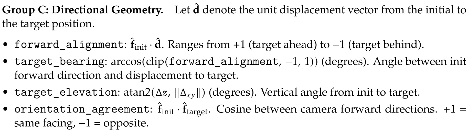
Group C: Directional Geometry.
Directional factors measure forward alignment with target displacement, target bearing, target elevation and agreement between camera forward axes. Their exact definitions are retained; interpretation of signed alignment/bearing depends on resolving the stated forward-axis convention.
Original selectable text and notation
Let denote the unit displacement vector from the initial to the target position.
- •
forward_alignment: . Ranges from (target ahead) to (target behind).
- •
target_bearing: (degrees). Angle between init forward direction and displacement to target.
- •
target_elevation: (degrees). Vertical angle from init to target.
- •
orientation_agreement: . Cosine between camera forward directions. = same facing, = opposite.
Appendix C Iterative Training Implementation Details
C.1 Algorithm
Algorithm 3 alternates PPO exploration, persistent graph accumulation, path reformulation and supervised updates. The returned policy has learned from both rewarded goals and relabeled transitions.
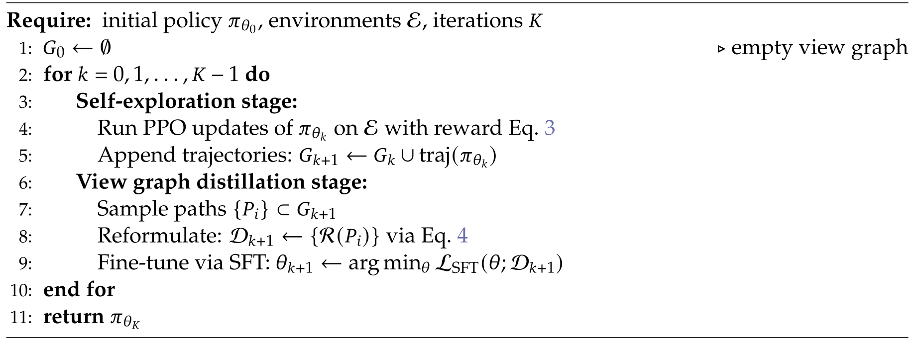
Original selectable algorithm
C.2 RL Hyperparameters
Table 11 specifies actor/critic learning rates of 10⁻⁶/10⁻⁵, GAE, batch size 128, FSDP offloading, checkpointing and asynchronous SGLang rollouts on eight GPUs. Maximum prompt/response lengths are 4,000/10,000 tokens.
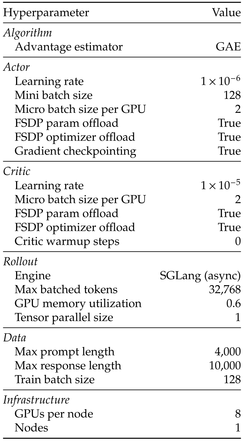
Original selectable table
| Hyperparameter | Value |
| Algorithm | |
| Advantage estimator | GAE |
| Actor | |
| Learning rate | |
| Mini batch size | 128 |
| Micro batch size per GPU | 2 |
| FSDP param offload | True |
| FSDP optimizer offload | True |
| Gradient checkpointing | True |
| Critic | |
| Learning rate | |
| Micro batch size per GPU | 2 |
| FSDP param offload | True |
| FSDP optimizer offload | True |
| Critic warmup steps | 0 |
| Rollout | |
| Engine | SGLang (async) |
| Max batched tokens | 32,768 |
| GPU memory utilization | 0.6 |
| Tensor parallel size | 1 |
| Data | |
| Max prompt length | 4,000 |
| Max response length | 10,000 |
| Train batch size | 128 |
| Infrastructure | |
| GPUs per node | 8 |
| Nodes | 1 |
Iteration-specific overrides.
Iterations 0–2 each use sixty RL steps for bootstrapping; iteration 3 runs to convergence. The final step count and a matched total training-cost comparison are not specified here.
Direct GRPO baseline.
The filtered direct-GRPO baseline replaces GAE with group-relative advantages, uses four rollouts per prompt and trains for 1,000 steps under the same infrastructure.
C.3 SFT Hyperparameters
SFT uses learning rate 10⁻⁵, cosine scheduling, 0.01 weight decay, 0.1 warm-up ratio, BF16, FlashAttention 2 and DeepSpeed ZeRO-2, with 16,384-token cutoff and a 20% validation split. Table 12 lists three epochs for iterations 0–2 and four for iteration 3; Table 13’s caption instead calls the final iteration RL-only. This schedule discrepancy is left unresolved.
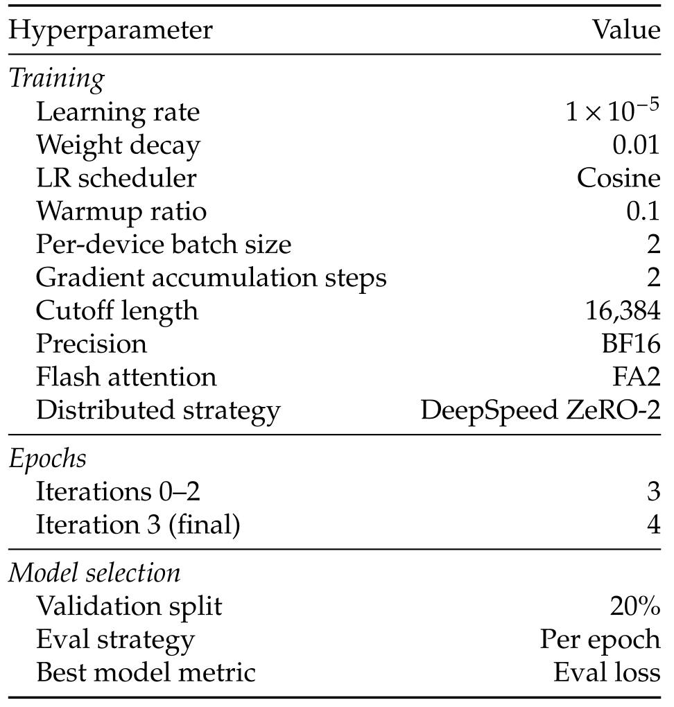
Original selectable table
| Hyperparameter | Value |
| Training | |
| Learning rate | |
| Weight decay | 0.01 |
| LR scheduler | Cosine |
| Warmup ratio | 0.1 |
| Per-device batch size | 2 |
| Gradient accumulation steps | 2 |
| Cutoff length | 16,384 |
| Precision | BF16 |
| Flash attention | FA2 |
| Distributed strategy | DeepSpeed ZeRO-2 |
| Epochs | |
| Iterations 0–2 | 3 |
| Iteration 3 (final) | 4 |
| Model selection | |
| Validation split | 20% |
| Eval strategy | Per epoch |
| Best model metric | Eval loss |
C.4 View Graph Construction
A concurrent background process merges completed rollouts into the view graph. Persisting experience enables later stages to revisit transitions collected before the policy improved.
Node and edge representation.
Nodes store a six-degree-of-freedom pose and 512×512 render; directed edges store the intervening camera-action sequence. Views are rejected if more than 70% is void or pixel standard deviation is below ten, removing outside-scene and nearly uniform observations.
Deduplication.
Nodes within 0.25 m and 15° are merged, redirecting incident edges. Duplicate edges share source, target and action sequence. This controls redundant growth, but proximity is not identity: replaying redirected/composed actions from the merged pose can differ from their original endpoint. No error bound or replay validation for these merged paths is described.
Cross-iteration accumulation.
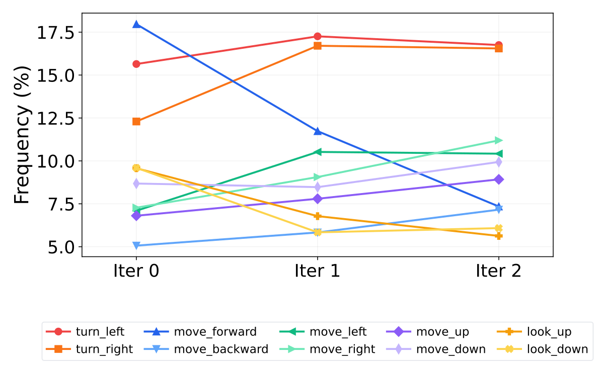
The graph grows from 4,067 nodes/2,875 edges in 186 scenes to 61,862/62,445 and then 66,492/65,577 in 193 scenes. Average actions per edge remain about 1.5–1.7. Figure 11 shows the policy shifting from frequent forward moves toward more turns and balanced translations; action frequency alone does not measure planning quality.

Original selectable table
| Iteration | Scenes | Nodes | Edges | Avg Nodes/Scene | Avg Actions/Edge |
|---|---|---|---|---|---|
| 0 | 186 | 4,067 | 2,875 | 21.9 | 1.6 |
| 1 | 193 | 61,862 | 62,445 | 320.5 | 1.5 |
| 2 | 193 | 66,492 | 65,577 | 344.5 | 1.7 |
C.5 Task Reformulation Details
Table 14 retains the three sampled supervision types and per-scene counts. The graph is a shared data source; not all suggested reformulations are used in the experiments.

Original selectable table
| Task Type | Path Length | Samples/Scene | Balanced |
|---|---|---|---|
| Multi-turn view planning | 3–5 | 20 | No |
| View-difference estimation | 2–5 | 15 | Yes |
| View-difference MCQ | 2–5 | 15 | Yes |
Multi-turn view planning (primary task).
Paths of three to five graph edges provide intermediate observations and actions, with the endpoint relabeled as target. Each path is sampled ten times with different seeds; the table specifies twenty samples per scene before this stated oversampling. Edge count differs from action count because one edge can store several actions.
View-difference estimation.
Pairs separated by two to five graph edges train prediction of the geometric unified view distance. Balanced path-length sampling supplies fifteen samples per scene. Graph path length selects examples but is not itself the distance target.
View-difference MCQ.
A second auxiliary task expresses the same view-distance question as four-choice selection, also with fifteen balanced samples per scene. This varies output format while sharing geometric supervision.
Additional reformulations (not used in main experiments).
Inverse dynamics could predict an action sequence between views, while forward dynamics could predict the resulting view. Both are proposed future reformulations; their training effects are not evaluated.
C.6 Training and Validation Environments
Training and validation are defined by viewpoint pairs within the scene splits. The count of pair-defined environments should not be confused with the number of distinct reconstructed scenes.
Training.
RL uses 3,419 training view pairs, each specifying a scene, initial view and target view. Episodes allow ten turns and render at 512×512 through Open3D.
Validation.
Validation contains 378 P2V instances, 378 V2P instances and 100 IVP instances. These are separate from the 530-pair test evaluation.
Appendix D Extended Analysis
D.1 Point Cloud Coverage: Full Model Comparison
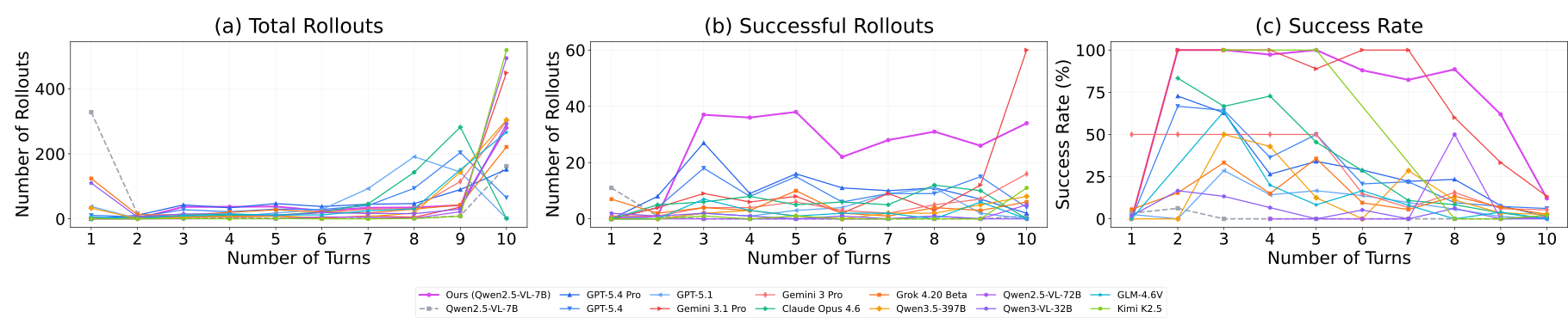
Figure 12 extends the coverage comparison to the full plotted model set. The trained model reaches higher aggregate target coverage; neither the source’s monotonicity wording nor a decline in another aggregate curve establishes the behavior of every individual rollout.
Methodology.
Scene coverage divides the cumulative visible-vertex union by all scene vertices; target coverage intersects that union with vertices visible from the target and normalizes by the target set. Means exclude late turns represented by fewer than 1% of the maximum rollout count; shading is ±1 standard deviation, not a confidence interval. Early termination changes the contributing cohort, explaining how aggregate cumulative-coverage curves can fall even though each fixed trajectory’s union cannot shrink.

Original selectable text and notation
- •
Scene coverage ratio: , where is the set of vertices visible at turn and is the full scene point cloud.
- •
Target intersection ratio: , where is the set of vertices visible from the ground-truth target viewpoint.
Turn distribution and success rate.
The base Qwen model and GPT-5.4 Pro often stop immediately; trained Qwen and Gemini commonly consume the full budget. Trained success is high among short episodes and lower among long ones. These condition-on-stopping-time curves mix task difficulty with behavior and are not a controlled effect of granting more turns.
D.2 Attention Analysis: Methodology and Full Results
Figure 5 retains all 28 layer plots. Both policies are evaluated on the same trajectories, making the attention comparison more controlled than comparing their separately generated histories.
Setup.
For each response token, image attention is the sum of attention to image-token positions divided by attention to all positions, , averaged over response tokens and heads. Rollouts with fewer than three images or no response tokens are excluded; error bars are ±1 standard deviation across trajectories.
Implementation.
All layers use eager softmax attention. To fit histories with up to roughly 6,000 tokens and twelve images, the implementation tiles the query dimension and reduces each tile directly to image-attention fractions. It therefore reports all layers from one consistent forward pass, rather than changing attention computation between models.
D.3 Spatial Prior Transfer: Post-Training Details
Both initializations receive further GRPO on jointly trained P2V/V2P and separately on MindCube. Matching downstream data and steps tests whether the prior helps adaptation; it does not show an untrained transfer gain.
Training hyperparameters.
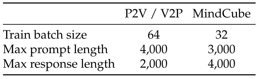
Post-training runs 401 steps on eight GPUs, with eight rollouts per prompt, actor learning rate 10⁻⁶ and no KL penalty. Table 15 gives batches 64/32 and prompt/response limits 4,000/2,000 versus 3,000/4,000 for P2V/V2P and MindCube respectively.
Reward functions.
Rewards combine valid formatting with a case-insensitive first-character answer check. P2V/V2P weight format/answer by 0.1/0.9; MindCube uses 0.2/0.8. The retained definitions make this a mixture of binary component rewards, not a single binary total.
