At a glance
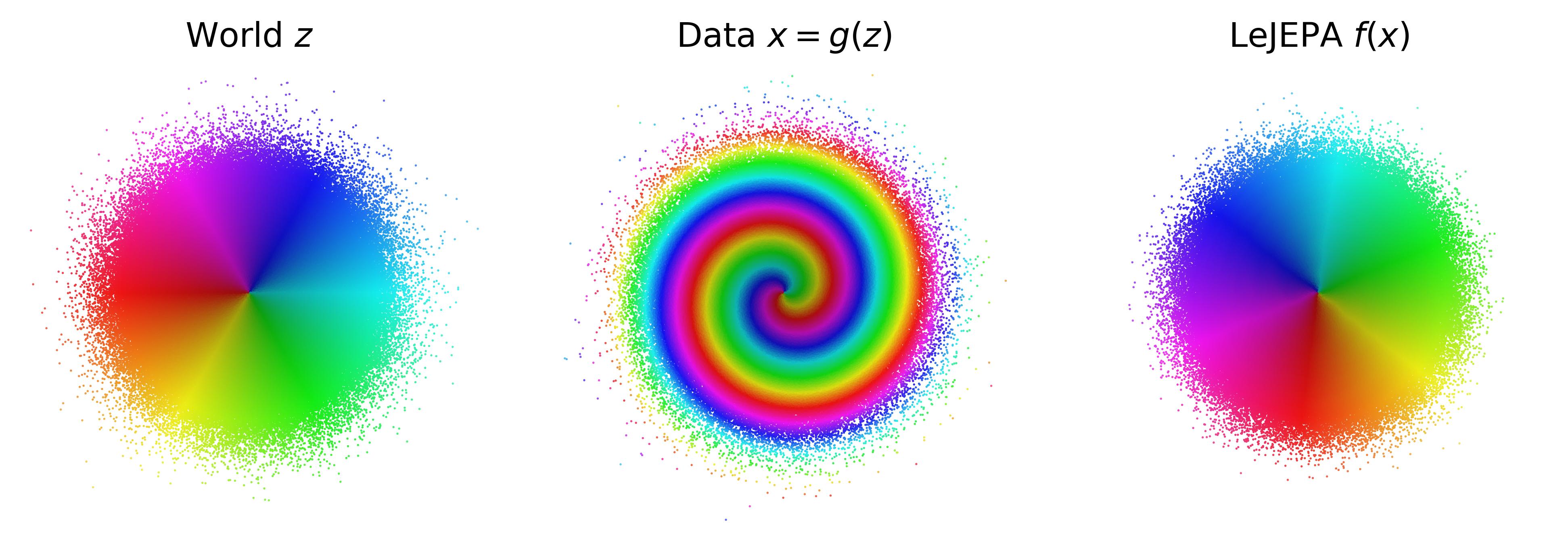
Intuition. A map can preserve enough information for a classifier yet twist positions so that a straight line in the map becomes a curved path in the real world. This paper asks when a learned representation recovers the hidden state through only a rotation or reflection. Such a coordinate change preserves Euclidean distances and simplifies planning.
The guarantee concerns a specific world: independent Gaussian latent variables, stationary isotropic noisy transitions, matched latent/output dimension and an ideal population objective. The paper also studies approximate optimization and violations of these assumptions. Its Gaussian-uniqueness claim is within the stated world class, not a claim that other worlds cannot be learned by any method.
1 Introduction
The central question is identifiability: which hidden-state descriptions are determined by observations, positive-pair structure and the learning objective? Good downstream classification alone cannot determine this. The desired result is a learned coordinate system related linearly—and, here, orthogonally—to the true latent state.
Contributions.
The paper combines a forward recovery theorem, a converse within a specified transition family, an approximate-error bound and a coordinate-equivalence result for planning. Controlled experiments test each claim and separately explore natural images, extra predictors and incorrect output dimension.
2 Related Work
Representation Learning.
JEPA methods encourage related observations to agree while avoiding constant representations. This study compares different regularizers but focuses on which underlying state variables can be recovered, rather than treating probe accuracy as a complete world-model definition.
World Models.
World models span prediction, control and generative simulation. This result chiefly addresses the encoder’s state coordinates. Learning accurate action-conditioned dynamics and choosing a successful numerical planner remain additional problems.
Identifiability.
Identifiability needs structure in the data-generating process or learning problem. The study connects JEPA to slow-feature and independent-component analysis, while allowing broad measurable representation maps in its idealized analysis.
3 The World and the Learner
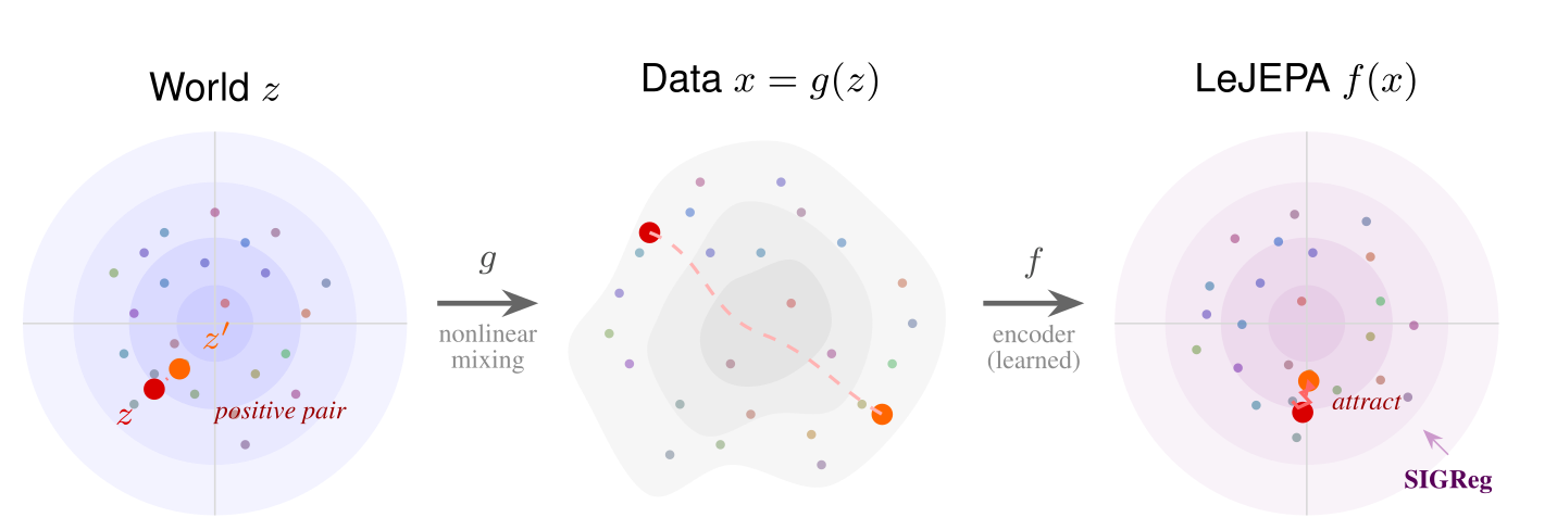
The world has hidden variables z, and an unknown observation process produces x. The encoder maps x to a learned state. Linear identifiability means the learned state retains the true state up to a linear coordinate change. It does not attach unique human names to individual coordinates.
3.1 The World
The setup specifies independent latent coordinates, stationary positive pairs and independent additive-noise transitions. These are modeling assumptions about how paired observations are generated. Ordinary adjacent robot frames need not satisfy them.
Assumptions (World)
Independence. and transitions for all .
Stationarity. Both views share the same marginal: .
Additive noise. with independent of .
3.1.1 The Gaussian World
The Gaussian case uses a common correlation parameter between zero and one for all coordinates: the next state is a contracted current state plus independent Gaussian noise of the matching variance. This preserves the standard Gaussian marginal. Equal transition scales are important to the spectral argument.
Equation 1
| (1) |
3.2 The Learner: LeJEPA
The analyzed LeJEPA learner minimizes paired-state disagreement while keeping embedding covariance or distribution nondegenerate, with output dimension matching the latent dimension. Exact population optimality is an idealization. The theorem does not supply an optimization algorithm guaranteed to reach that optimum from finite pixels.
Equations 2–3
| (2) |
| (3) |
4 Spectral Analysis of the World
The proof studies which functions of state stay correlated across a transition. These are analogous to frequency components, but adapted to the stochastic world.
Transition Operator.
The transition operator maps a function to its expected value at the next state, given the current state. Its eigenfunctions describe independently evolving patterns. Large eigenvalues correspond to patterns that remain more correlated across positive pairs.
Gaussian World: Hermite Polynomials.
In the Gaussian world, Hermite polynomials play the role of a natural basis. Linear patterns retain correlation ρ, quadratic ones ρ² and higher degrees still less. Since 0 < ρ < 1, mixing in nonlinear components reduces the best achievable alignment under the stated normalization.
Equation 4
| (4) |
General Case: Sturm-Liouville Theory.
For the more general transition family, a Sturm–Liouville equation describes the slow features. Requiring its relevant eigenfunction to be affine places a strong condition on the latent density, leading to the Gaussian converse.
5 Theory
Four results connect the encoder geometry to the world and then to planning. The manuscript supplies Lean verification files, with standard background results explicitly axiomatized; this is not a claim that every background theorem or software dependency was independently audited here.
5.1 Forward Direction: LeJEPA Learns the World Model
At the ideal optimum in the specified Gaussian world, the representation recovers the latent coordinates up to an orthogonal map. The original formal statement is retained.
Proof Sketch.
The alignment objective becomes a sum of correlations. Each normalized coordinate reaches its maximum only when its Hermite expansion is linear. The covariance condition then forces the resulting linear matrix to be orthogonal.
Interpretation.
A global rotation or reflection preserves distances and the modeled transition. It may still mix what a person would call position, color or velocity; the result is not unique coordinate-by-coordinate semantic labeling.
5.2 Converse Direction: The Gaussian is Unique
The converse concerns the specified stationary additive-noise world class. The slow eigenfunction must be affine for the desired linear recovery, and that condition selects a Gaussian latent density under the stated assumptions.
Proof Sketch.
Substituting an affine eigenfunction into the governing equation makes the derivative of log density linear. Integrating yields a quadratic log density, with normalizability selecting the Gaussian form.
5.3 Approximate Identifiability
An approximate result allows nonzero alignment error and covariance mismatch inside the same theoretical setting. It quantifies recovery error rather than assuming every trained checkpoint attains exact constraints.
Theorem 3 (Approximate Identifiability)
Consider the Gaussian world (3.1.1). Let be measurable with , satisfying: Approximate alignment: ; Approximate whitening: . Define . Then there exists such that
Equation
Interpretation.
The bound separates nonlinear distortion from deviation of the linear part from orthogonality. Its dependence on the transition correlation matters; it is not a distribution-free guarantee for arbitrary non-Gaussian data.
5.4 Optimal Latent Planning
An orthogonal change of state coordinates preserves an equivalent control problem when dynamics and costs are transformed consistently. Rotation-invariant costs, such as Euclidean goal distance, are a convenient special case. This is a coordinate-equivalence theorem, not proof that a learned dynamics model or numerical optimizer is exact.
Theorem 4 (Optimal Latent Planning)
Let with , and let the costs be rotation-invariant:
Equation
Then planning in the learned latent , with transitions mapped through and the same costs, yields the same value and plan: and .
Interpretation.
Equivalent true and learned-coordinate problems have matching action sequences and values. Additional learning or planning errors can still make a practical controller depart from that ideal.
6 Experiments
Experiments move from controlled latent mixtures to pixels, then deliberately violate dimension, distribution or predictor assumptions. Those latter results are empirical extensions rather than automatic consequences of the main theorem.
6.1 Forward: Linear Identifiability from Gaussian Latent Variables
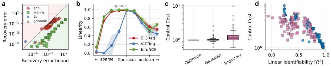
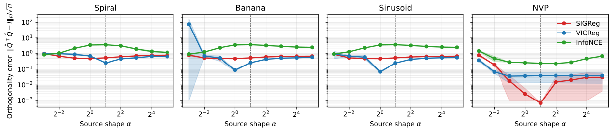
Four invertible nonlinear mixing functions turn Gaussian latent states into observations. LeJEPA learns to undo those mixings up to rotation. One mixing preserves the Gaussian marginal itself, showing why Gaussianity alone is insufficient: the positive-pair alignment provides additional structure.

| Mixing | Linear identifiability | |||
| SIGReg | VICReg | InfoNCE | ||
| std | std | std | std | |
| 2 | 0.7812.1 | 0.9999983.4 | 0.9999968.4 | 0.9509611.6 |
| 4 | 0.72724 | 0.99999612 | 0.99998754 | 0.9108718.2 |
| 8 | 0.72810 | 0.9999939.0 | 0.9999884.8 | 0.88681842 |
| 16 | 0.7346.3 | 0.9999884.9 | 0.9999874.6 | 0.9998800.01 |
| 32 | 0.7372.3 | 0.9999817.2 | 0.9999819.4 | 0.90780926 |
| 64 | 0.7371.5 | 0.9999667.4 | 0.9999688.1 | 0.6484963.1 |
| 128 | 0.7390.61 | 0.9999383.2 | 0.9999427.2 | 0.5669556.6 |
| 256 | 0.7420.49 | 0.9998847.9 | 0.9998897.2 | 0.6965870.49 |
| 512 | 0.7490.30 | 0.9997756.7 | 0.9997856.9 | 0.7043930.26 |
| 1024 | 0.7630.17 | 0.99956112 | 0.99958211 | 0.7202410.20 |
| 2048 | 0.7680.05 | 0.9990437.9 | 0.9990947.5 | 0.7271400.10 |
| 4096 | 0.7680.03 | 0.663 0.999449† | 0.652 | 0.7271110.02 |
Scaling to High Dimensions.
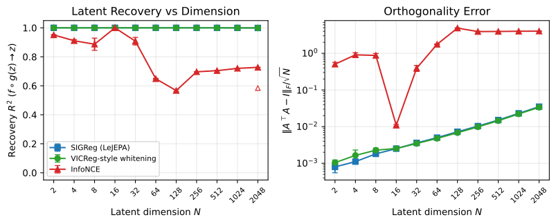
Scaling experiments increase latent dimension through 4096 and compare SIGReg, VICReg and InfoNCE. Larger dimensions expose finite-batch and kernel-width limitations. Increasing the batch restores strong SIGReg recovery in the largest tested case, separating estimation issues from the population identifiability statement.
6.2 Converse: Non-Gaussian Latent Variables Break Linear Identifiability
The next tests change the latent distribution and sampling process to examine where linear recovery weakens.
| OU (Gaussian) | Trajectory (non-Gaussian) | |||||||
|---|---|---|---|---|---|---|---|---|
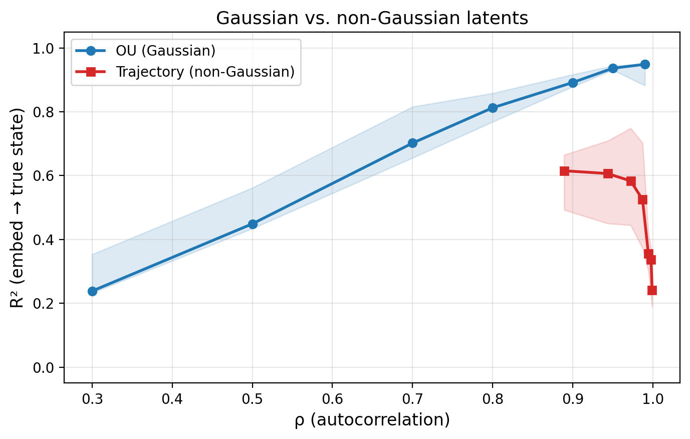
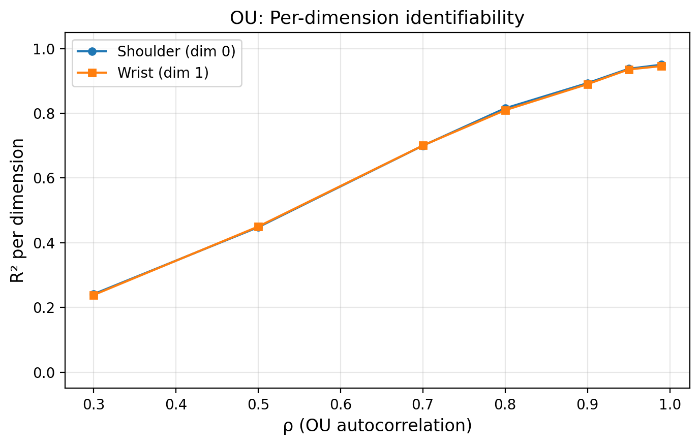
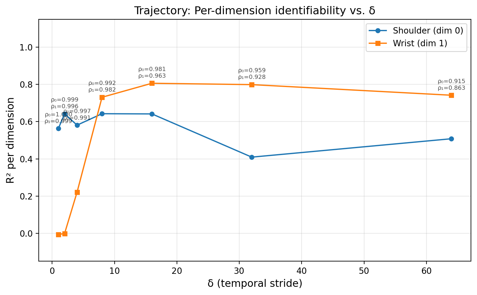
| 0.30 | 0.672e-02 | 0.672e-02 | 1 | 1.000 | 0.999 | -0.391e-01 | 0.713e-02 | -0.034e-02 |
| 0.50 | 0.861e-02 | 0.861e-02 | 2 | 0.999 | 0.996 | -0.475e-02 | 0.734e-03 | 0.012e-03 |
| 0.70 | 0.937e-03 | 0.937e-03 | 4 | 0.997 | 0.991 | -0.053e-01 | 0.511e-01 | 0.439e-02 |
| 0.80 | 0.943e-04 | 0.943e-04 | 8 | 0.992 | 0.982 | 0.502e-02 | 0.802e-03 | 0.786e-03 |
| 0.90 | 0.957e-04 | 0.957e-04 | 16 | 0.981 | 0.963 | 0.444e-02 | 0.632e-02 | 0.872e-02 |
| 0.95 | 0.952e-04 | 0.952e-04 | 32 | 0.959 | 0.928 | 0.456e-02 | 0.622e-02 | 0.811e-02 |
| 0.99 | 0.954e-04 | 0.954e-04 | 64 | 0.915 | 0.863 | 0.444e-02 | 0.553e-02 | 0.772e-02 |
Latent-Distribution Sweep.
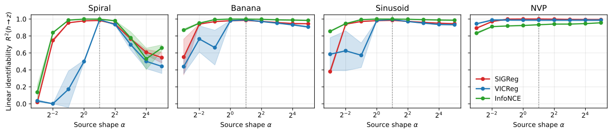
A generalized-normal sweep varies the latent shape from heavy-tailed through Gaussian toward uniform. Recovery is strongest near the Gaussian setting under the tested transitions and objectives.
Pixel-Based RL Trajectories.
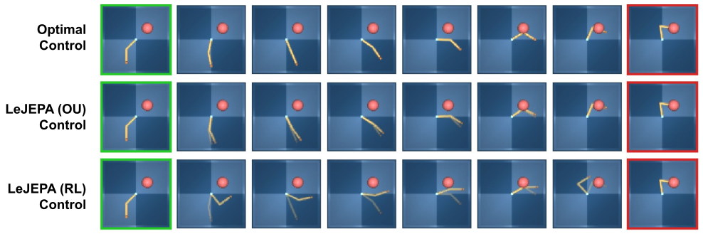
The Reacher experiment uses the same image renderer with either controlled Gaussian transitions or recorded policy trajectories. The latter violate several assumptions at once, including marginal shape, isotropic correlation and joint-limit behavior. Their weaker recovery cannot isolate non-Gaussianity as the only causal change.
6.3 Approximation Bound and Loss Predict Identifiability
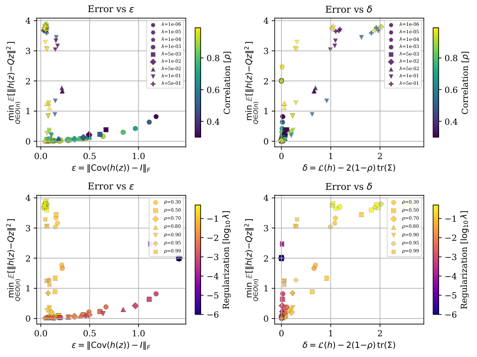
Measured alignment gap and covariance mismatch are compared with recovery error under controlled runs. Loss can be a useful proxy in these settings, but estimating the bound itself needs the theoretical quantities and finite-sample care.
6.4 Linear Identifiability Enables Latent-Space Planning
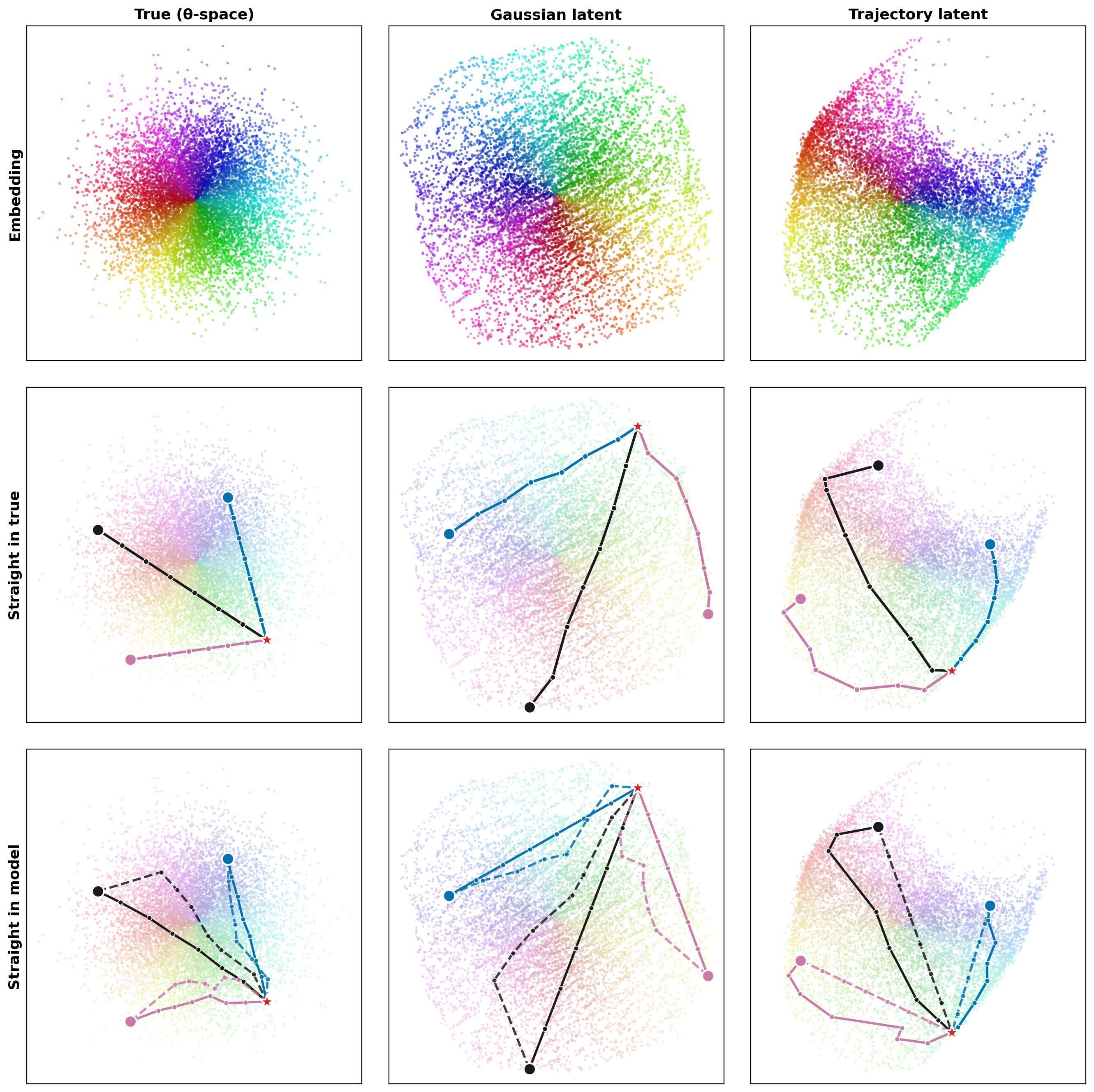
Straight-line plans in a faithfully recovered latent space correspond closely to straight paths in the true joint space. Distorted representations produce curved or more costly paths. The experiment evaluates this particular goal-reaching geometry, not every robotic planning task.
6.5 Beyond the Assumptions: Latent Dimension, Natural Images, Predictors
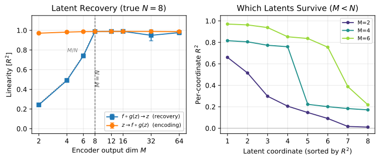
Unknown latent dimension.
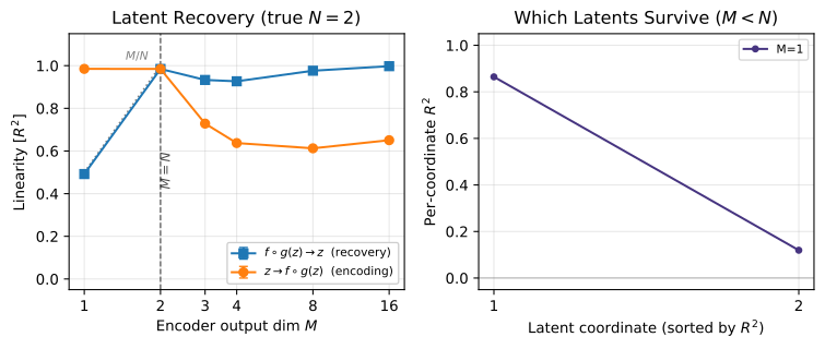
Too few output coordinates retain only a subspace in the tested setting; larger outputs eventually saturate recovery. Covariance participation ratio is explored as a dimension diagnostic. Its behavior here does not make intrinsic dimension universally identifiable from arbitrary embeddings.
Natural images.
ImageNet-X factors are linearly probed in pretrained visual encoders. These empirical comparisons test observable factor information without access to the true generative state, so they do not verify all Gaussian-world assumptions on natural images.
Predictors.
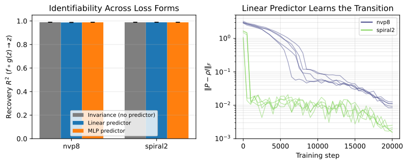
Adding a learned linear or multilayer predictor preserves recovery in the tested controlled experiments. A sufficiently flexible predictor could absorb an encoder distortion, so the general nonlinear-predictor extension remains empirical here.
7 Limitations
Are the latents Gaussian?
Real latent factors need not be independent, Gaussian or Euclidean. Maximum-entropy and aggregation arguments motivate a prior but do not establish those properties from observations. Extending the theory to other worlds remains open.
Finite samples and optimization.
The results concern a population optimum, not sample-complexity or training-convergence guarantees. The approximation theorem controls stated errors inside its setup; finite-sample estimates can introduce apparent bound violations.
8 Discussion
Outlook.
Actions, interventions and learned dynamics introduce further questions beyond encoder recovery. Inverse dynamics may help retain controllable factors in settings not covered by the passive Gaussian argument.
Practical Implications.
The experiments suggest that data collection and objective estimation both affect recovery. Goal-directed trajectories and isotropic exploration can expose different parts of the same physical state space. No one regularizer is established as optimal across every data regime.
A Theoretical Foundation for World Models.
The useful contribution is a conditional link between representation geometry and equivalent control coordinates. Keep the world assumptions, encoder guarantee and additional dynamics-learning problem separate when applying it.
Acknowledgments
The authors acknowledge feedback, computing support and funding.
Appendix Overview
The appendices contain notation, proofs, connections to slow features, Lean verification scope and detailed experimental settings.
| Contents | Page | |
|---|---|---|
| Appendix A | Proof of Thm. 5.1 (linear identifiability), incl. Hermite background | A |
| Appendix B | Proof of Thm. 5.2 (Gaussian uniqueness) | B |
| Appendix C | Proof of Thm. 5.3 (approximate identifiability) | C |
| Appendix D | Proof and discussion of Thm. 5.4 (optimal latent planning) | D |
| Appendix E | Alternative proof via Dirichlet energy | E |
| Appendix F | Prior work: connection to Slow Feature Analysis | F |
| Appendix G | Lean 4 formal verification | G |
| Appendix H | Experimental details and additional results | H |
| Symbol | Description |
|---|---|
| World Model | |
| True latent variables and positive pair (second view) | |
| -th coordinate of , one scalar latent variable | |
| Latent dimension | |
| Encoder output dimension ( in theorems; App. H.13) | |
| Deterministic part of the additive-noise transition, | |
| Autocorrelation of the Ornstein–Uhlenbeck transition, | |
| Independent transition noise | |
| Diffusion coefficient (Sturm–Liouville setting) | |
| Maps | |
| Unknown nonlinear mixing (generative) function; | |
| Learned encoder; | |
| Composed map from latent space to representation space | |
| Jacobian matrix of at | |
| Linear algebra | |
| Orthogonal group (matrices with ) | |
| Orthogonal recovery matrix (exact identifiability) | |
| Losses and objectives | |
| Alignment loss: | |
| Empirical invariance (alignment) loss | |
| SIGReg Gaussianity regularizer | |
| Regularization weight balancing and | |
| Hermite polynomials and spectral decomposition | |
| Probabilist’s Hermite polynomial of degree | |
| Normalized Hermite polynomial: | |
| Multi-index ; is the total degree | |
| Multivariate Hermite basis function: | |
| Hermite coefficient of at multi-index | |
| Variance fraction of at degree : | |
| Transition operator: | |
| Approximate identifiability | |
| Alignment gap (excess loss above the linear optimum) | |
| Covariance deviation: | |
| Normalized alignment gap: | |
Appendix A Proof of Theorem 5.1 (Forward Direction)
A.1 Intuition: Why Should This Force Linearity?
An informal information argument motivates linearity but has gaps when transformed joint distributions are not Gaussian. The Hermite proof supplies the rigorous spectral route instead.
A.2 Hermite Polynomial Background
Definitions and orthogonality.
Hermite polynomials form an orthogonal basis for square-integrable functions under a Gaussian measure.
Equations 7–9
| (7) |
| (8) |
| (9) |
Multivariate extension.
Products of one-dimensional Hermite polynomials extend the basis to independent Gaussian coordinates, grouped by total degree.
Equation 10
| (10) |
Hermite expansion of measure-preserving maps.
Expansion coefficients divide each learned coordinate’s variance between linear and higher-degree components.
Equations 11–12
| (11) |
| (12) |
A.3 Proof
Setup and notation.
The proof rewrites normalized alignment as correlation and organizes each representation component by Hermite degree.
Equation 13
| (13) |
Step 1: The transition attenuates each Hermite degree by ρ d .
The Gaussian transition attenuates a degree d component by ρ to the power d, making higher degrees less persistent.
Equations 14–21
| (14) |
| (15) |
| (16) |
| (17) |
| (18) |
| (19) |
| (20) |
| (21) |
Step 2: Different Hermite components do not interact across views.
Orthogonality eliminates cross-terms between distinct basis components across the two views.
Equations 22–24
| (22) |
| (23) |
| (24) |
Step 3: Nonlinearity strictly reduces correlation.
Any nonzero higher-degree variance therefore reduces the attainable correlation relative to a linear component.
Equations 25–28
| (25) |
| (26) |
| (27) |
| (28) |
Step 4: Assembly.
At equality every coordinate is linear, and the covariance constraint makes the combined matrix orthogonal.
Equation 29
| (29) |
Step 5: Recovery of the transition.
Substitution shows that an orthogonal coordinate change preserves the specified Gaussian transition law.
Appendix B Proof of Theorem 5.2 (Gaussian Uniqueness)
B.1 Background
The converse uses the diffusion generator and its eigenfunctions under the stated stationary density and boundary assumptions.
Equation 30
| (30) |
B.2 Proof
An affine slow eigenfunction forces a linear density score, selecting a Gaussian among the admissible latent laws.
Equations 31–33
| (31) |
| (32) |
| (33) |
Remark: the OU transition is a modeling choice.
The Ornstein–Uhlenbeck transition is a chosen world model. Gaussian marginals alone do not force every possible transition to have that form.
Appendix C Proof of Theorem 5.3 (Approximate Identifiability)
Setup and notation.
The approximate proof names separate alignment and whitening deviations before bounding recovery error.
Equations 35–38
| (35) |
| (36) |
| (37) |
| (38) |
C.1 Step 1: Alignment gap controls nonlinear energy
The spectral gap bounds how much variance can occupy nonlinear components when alignment is nearly optimal.
Equations 39–45
| (39) |
| (40) |
| (41) |
| (42) |
| (43) |
| (44) |
| (45) |
C.2 Step 2: Whitening constraint forces M near orthogonal
Covariance error and nonlinear energy bound how far the remaining linear matrix is from an orthogonal matrix.
Equations 46–48
| (46) |
| (47) |
| (48) |
C.3 Step 3: Pythagorean decomposition
Orthogonality separates the two error contributions to obtain the recovery bound.
Equations 49–52
| (49) |
| (50) |
| (51) |
| (52) |
Role of the Gaussian on the latent side vs. the output side.
Gaussian latent transitions support the spectral argument; approximate output whitening is a different condition and cannot replace the latent-world assumptions.
Appendix D Proof and Discussion of Theorem 5.4
Theorem 5.4 (Optimal Latent Planning)
Let with , write , and consider any finite-horizon optimal control problem whose stage and terminal costs are -invariant in the state argument:
Equation
Let denote the pushforward of under , and let denote the value function and optimal plan of the -space problem defined by replacing with and leaving costs unchanged. Then and .
Equations 54–55
| (54) |
| (55) |
D.1 Worked Applications
Goal-reaching.
Euclidean goal-reaching costs are unchanged by the same orthogonal transformation of states and goals.
Linear-quadratic regulation.
Linear-quadratic control transfers by consistently changing state matrices and cost coordinates.
Equations 56–58
| (56) |
| (57) |
| (58) |
General rotation-invariant objectives.
More general objectives transfer through coordinate transformation; rotation-invariant ones need no changed functional form.
D.2 Scope: encoder versus action-conditioned dynamics
Encoder identifiability does not by itself train the action-conditioned transition or eliminate model error.
D.3 Connection to classical optimal control
The planning statement is a change-of-coordinates result for classical control applied after representation learning.
Appendix E Alternative Proof via Dirichlet Energy
E.1 Setup
The alternative argument studies a small-transition, differentiable regime using Dirichlet energy.
Equation 59
| (59) |
E.2 Proof
Theorem 5 (Identifiability via Dirichlet energy)
Any diffeomorphism that preserves the standard Gaussian measure and minimizes must satisfy for some orthogonal matrix .
Step 1: Reduction to Dirichlet energy.
A small-step expansion relates paired-state disagreement to a gradient-energy functional.
Equations 60–64
| (60) |
| (61) |
| (62) |
| (63) |
| (64) |
Step 2: The expected log-determinant is zero.
The change-of-variables calculation controls the expected Jacobian log determinant under its stated regularity assumptions.
Equations 65–66
| (65) |
| (66) |
Step 3: Lower bound via AM-GM and Jensen.
Arithmetic–geometric mean and convexity inequalities establish the energy lower bound.
Equations 67–69
| (67) |
| (68) |
| (69) |
Step 4: Equality forces orthogonal Jacobian.
Equality requires an orthogonal local Jacobian rather than arbitrary nonlinear stretching.
Equation 70
| (70) |
Step 5: Orthogonal Jacobian implies linearity (Mazur–Ulam).
A rigidity argument turns the relevant distance-preserving structure into a global affine/orthogonal map.
Equations 71–73
| (71) |
| (72) |
| (73) |
Generalization.
The extension is limited by the alternative proof’s differentiability and small-transition conditions.
E.3 Comparison of the Two Proofs
The Hermite proof handles the stated finite-correlation Gaussian setting; the energy proof offers a complementary, more restrictive route.
| Hermite proof | Dirichlet energy proof | |
|---|---|---|
| Regularity | Measurable | diffeomorphism |
| Noise level | Any | Infinitesimal () |
| Key tool | Mehler’s formula | AM-GM + Jensen + Mazur–Ulam |
| Mechanism | Low-pass filter on degrees | Jacobian rigidity |
| Connection to | Harmonic analysis | Differential geometry |
Appendix F Prior Work: Connection to Slow Feature Analysis
SFA and its optimization problem.
Slow-feature analysis favors functions that vary least across related states while preventing trivial constants.
Nonlinear identifiability via SFA.
For general worlds, slow features can identify a source only through a nonlinear monotone transformation.
Eigenfunction structure and Sturm–Liouville theory.
Sturm–Liouville structure orders the relevant one-dimensional diffusion eigenfunctions.
The Gaussian specialization and Hermite polynomials.
The Gaussian specialization yields Hermite modes with a tractable ordering by degree.
Sequential versus simultaneous extraction.
Sequentially extracting modes and jointly learning a multivariate representation impose different optimization constraints.
The role of isotropic transitions.
Equal transition scales prevent one coordinate’s nonlinear modes from outranking another coordinate’s linear mode.
Beyond Gaussian latents.
Other latent laws require a different recovery statement; the Gaussian result is not a universal nonlinear-ICA solution.
Relation to Mehler’s formula and maximal correlation.
Mehler’s formula and maximal-correlation facts explain the central preference for linear Gaussian modes.
Practical differences: learned features versus fixed kernels.
A learned neural representation differs from choosing fixed spectral features or a predefined kernel.
Connections to diffusion maps and spectral geometry.
Diffusion-map and spectral-geometry connections supply context for the transition-operator analysis.
Summary of the relationship.
The relationship concerns a shared preference for slow structure, with different assumptions determining what that structure represents.
| Sprekeler et al. (2014) | This work | |
|---|---|---|
| Identifiability class | Permutation | Orthogonal |
| Latent variable distributions | Any independent | Gaussian (or i.i.d. factorial) |
| Transition structure | Distinct rates required | Isotropic required |
| Extraction | Sequential (greedy) | Simultaneous |
| Function space | Fixed polynomial kernel | Learned (neural network) |
| Proof technique | Sturm–Liouville / PDE | Mehler’s formula / Parseval |
| Approximate bound | None | |
| Practical algorithm | xSFA (fragile, latent variables) | LeJEPA / SIGReg (scalable) |
Appendix G Lean Verification
Scope and methodology.
The verification files formalize the paper’s derivations relative to explicitly listed background assumptions.
| File / Component | Lean name | Status |
| Hermite.lean: Thm. 5.1 via Hermite polynomials | ||
| Hermite basis completeness | mehler_summability | axiomatized |
| Contraction lemma ( decay) | (folded into above) | axiomatized |
| Mehler’s formula | correlation_eq_spectral_sum | axiomatized |
| for | pow_le_self_of_pos_lt_one | verified |
| for (strict) | pow_lt_self_of_ge_two | verified |
| Pointwise bound | spectral_term_le | verified |
| Correlation bound (4) | correlation_le_rho | verified |
| Equality | equality_forces_degree_one | verified |
| Degree-1 linearity | linear_of_degree_one | axiomatized |
| Gaussianity + linear orthogonal | orthogonal_of_gaussian_linear | axiomatized |
| Loss lower bound | loss_lower_bound | verified |
| Theorem assembly | hermite_identifiability | verified |
| Uniqueness.lean: Thm. 5.2 (Gaussian uniqueness) | ||
| Affine eigenfunction affine score | score_affine_of_eigenfunction | verified |
| Affine score Gaussian density | gaussian_of_affine_score | axiomatized |
| Only-if direction assembly | gaussian_of_affine_eigenfunction | verified |
| Gaussian Hermite eigenfunctions | hermite_first_eigenfunction_of_gaussian | axiomatized |
| Full biconditional | gaussian_uniqueness | verified |
| Zero-mean specialization | score_pure_linear_zero_mean | verified |
| Dirichlet.lean: Appendix E via Dirichlet energy | ||
| AM-GM inequality | amgm_sum_ge_prod_pow | axiomatized |
| Jensen’s inequality (exp) | exp_mean_ge_mean_exp | axiomatized |
| Mazur–Ulam theorem | mazur_ulam | axiomatized |
| Norm-preserving CLM isometry | clm_isometry_of_norm_preserving | verified |
| Orthogonal Jacobian 1-Lipschitz | lipschitz_of_orthogonal_jacobian | verified |
| Bilipschitz global isometry | isometry_of_bilipschitz | verified |
| linear isometry | (part of assembly) | verified |
| Theorem assembly | dirichlet_identifiability | verified |
| Approx.lean: Thm. 5.3 (approximate bound) | ||
| Spectral gap positivity | spectral_gap_pos | verified |
| from alignment gap | nonlinear_energy_le_D | verified |
| Polar decomposition bound | polar_bound_axiom | axiomatized |
| Pythagorean decomposition | pythagorean_axiom | axiomatized |
| bound | linear_deviation_sq_bound | verified |
| Monotonicity of | bound_monotone | verified |
| Full bound | approximate_identifiability | verified |
| Exact recovery () | exact_recovery_special_case | verified |
| Planning.lean: Thm. 5.4 (planning equivalence) | ||
| Orthogonal invariance definition | IsOrthogonalInvariant | verified |
| Stage pushforward | stage_pushforward | axiomatized |
| Terminal pushforward | terminal_pushforward | axiomatized |
| Per-step stage cost equivalence | stage_cost_equiv | verified |
| Terminal cost equivalence | terminal_cost_equiv | verified |
| Total cost equivalence (main step) | planning_equivalence | verified |
| Minimizer equivalence | minimizer_equivalence | verified |
| Value equivalence | value_equivalence | verified |
G.1 What Is Axiomatized and Why
1. Hermite polynomial infrastructure.
Hermite-basis completeness and standard polynomial facts are supplied as background infrastructure.
2. Sturm–Liouville spectral theory.
The verification assumes the stated Sturm–Liouville spectral facts from the literature.
3. Standard analysis results requiring API software engineering.
Some standard analysis results are axiomatized where the theorem-prover library interface would require additional work.
4. Measure-theoretic and matrix-analytic facts.
Measure-theoretic and matrix facts are included among the declared background assumptions.
5. Trajectory pushforward for expected costs.
Trajectory pushforward facts support the expected-cost equivalence in planning.
What is verified.
The derived conclusions are checked within that declared formal environment; axiomatized facts are not newly proved by the files.
G.2 Build Information
Build information records the theorem-prover environment needed to reproduce the verification.
Appendix H Experimental Details and Additional Results
H.1 Nonlinear Mixing Functions
The controlled mixing functions are explicitly defined so latent recovery can be measured against known ground truth.
H.2 Network Architecture and Training
Encoder architecture and optimizer settings separate model capacity from the identifiability claim.
Equation 74
| (74) |
H.3 Training Procedure
The training loop constructs positive pairs and combines alignment with the selected regularizer.
Equation 75
| (75) |
H.4 Hyperparameters
The hyperparameter tables define the actual runs and searches rather than a parameter-free training guarantee.
| Hyperparameter | 2D / Gennorm / Grid | Scaling |
|---|---|---|
| Optimizer | AdamW | AdamW |
| Learning rate | ||
| LR schedule | warmup (10k) + cosine (10k) | warmup (10k) + cosine (10k) |
| Weight decay | 0 | 0 |
| Batch size | 256 | 256 |
| Training steps | 20,000 | 20,000 |
| Data regime | online (infinite) | online (infinite) |
| Eval points | 10,000 (fixed) | 10,000 (fixed) |
| Views per sample | 2 | 2 |
| 0.95 (2D/Gennorm), swept (Grid) | 0.95 | |
| (2D/Gennorm), swept (Grid) | ||
| Encoder | MLP (spiral/banana/sinusoid) | matched inverse-NVP [85] |
| matched NVP (nvp mixing) | ||
| Hidden dimension | 256 (MLP) | — |
| MLP layers | 4 | — |
| NVP coupling layers | 8 (2D/Gennorm) | 4 |
| Activation | GELU (MLP) | tanh (NVP) |
H.5 Evaluation Metrics
Metrics distinguish linear recovery, orthogonal recovery, covariance error and planning cost.
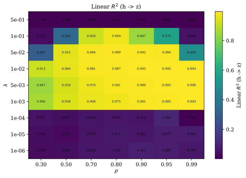
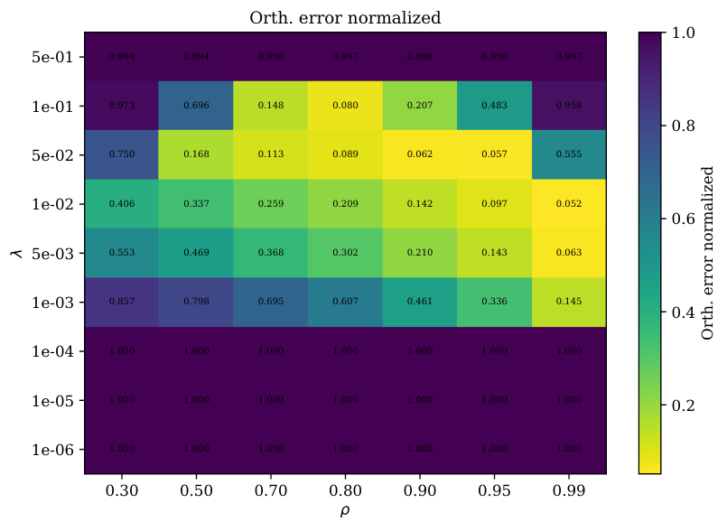
H.6 Grid Search
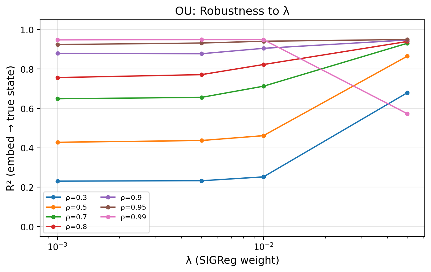
The grid search varies loss balance and transition correlation, exposing optimization-sensitive regimes.
H.7 Latent Variable Distribution Sweep Across Mixings
Distribution sweeps test the Gaussian optimum across controlled non-Gaussian alternatives and mixings.
H.8 Approximate Bound Decomposition
The bound decomposition compares nonlinear error and covariance distortion with measured recovery.
H.9 Loss Predictivity
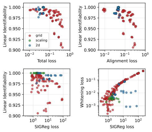
Training-loss predictivity is assessed across the stated runs; it remains an empirical checkpoint-selection signal.
SIGReg does not vanish at the optimum.
Finite-sample SIGReg can remain nonzero at an ideal population target, so a residual penalty need not imply equivalent representation error.
H.10 Scaling Experiment
The scaling study varies latent dimension with matched mixing and encoder capacity.
| Latents | Mixing difficulty | Linear identifiability | Orthogonality | SIGReg losses | |||
|---|---|---|---|---|---|---|---|
| Align | SIGReg | ||||||
| std | std | std | std | std | std | std | |
| 0.8711.4 | 0.7822.8 | 0.999993.4 | 0.999993.4 | 0.00024 | 0.047215 | 2.541.4 | |
| 0.86516 | 0.72424 | 0.9999912 | 0.9999912 | 0.00112 | 0.047510 | 2.091.3 | |
| 0.8604.2 | 0.72910 | 0.999999.0 | 0.999999.0 | 0.00114 | 0.047313 | 2.060.78 | |
| 0.8586.9 | 0.7336.0 | 0.999984.9 | 0.999984.9 | 0.00218 | 0.04763.6 | 1.760.18 | |
| 0.8513.0 | 0.7381.6 | 0.999987.2 | 0.999987.2 | 0.0037.6 | 0.04795.0 | 1.930.17 | |
| 0.8541.5 | 0.7371.4 | 0.999967.6 | 0.999967.4 | 0.00510 | 0.04843.9 | 2.030.14 | |
| 0.8530.62 | 0.7390.50 | 0.999933.1 | 0.999933.2 | 0.0077.4 | 0.04861.2 | 1.800.09 | |
| 0.8550.30 | 0.7420.48 | 0.999887.7 | 0.999887.9 | 0.0105.0 | 0.04862.9 | 1.880.17 | |
| 0.8590.24 | 0.7490.30 | 0.999776.5 | 0.999776.7 | 0.0153.7 | 0.04892.4 | 1.930.08 | |
| 0.8660.10 | 0.7630.17 | 0.9995612 | 0.9995612 | 0.0234.7 | 0.04880.91 | 1.930.06 | |
| 0.8690.03 | 0.7680.05 | 0.999048.1 | 0.999047.9 | 0.0351.5 | 0.04910.48 | 1.880.07 | |
| 0.8690.04 | 0.7680.02 | 0.999451.7 | 0.999441.9 | 0.0260.90 | 0.04890.14 | 1.910.11 | |
| Latents | Mixing difficulty | Linear identifiability | Orthogonality | VICReg losses | |||
|---|---|---|---|---|---|---|---|
| Align | Whitening | ||||||
| std | std | std | std | std | std | std | |
| 0.8710.66 | 0.7821.7 | 0.999998.4 | 0.999998.4 | 0.00119 | 0.049124 | 0.002213 | |
| 0.86515 | 0.72624 | 0.9999854 | 0.9999854 | 0.00165 | 0.047611 | 0.004113 | |
| 0.8694.4 | 0.7318.1 | 0.999984.9 | 0.999984.8 | 0.00231 | 0.047613 | 0.004512 | |
| 0.8606.9 | 0.7335.9 | 0.999984.7 | 0.999984.6 | 0.00212 | 0.04763.6 | 0.00362.8 | |
| 0.8551.5 | 0.7361.9 | 0.999989.4 | 0.999989.4 | 0.0033.6 | 0.04776.7 | 0.00353.3 | |
| 0.8531.7 | 0.7371.4 | 0.999968.2 | 0.999968.1 | 0.0049.0 | 0.04882.1 | 0.00351.8 | |
| 0.8530.87 | 0.7390.66 | 0.999947.1 | 0.999947.2 | 0.0069.5 | 0.04870.99 | 0.00350.75 | |
| 0.8550.25 | 0.7420.49 | 0.999887.2 | 0.999887.2 | 0.0094.1 | 0.04862.9 | 0.00350.39 | |
| 0.8580.23 | 0.7490.30 | 0.999787.2 | 0.999786.9 | 0.0143.7 | 0.04892.4 | 0.00350.29 | |
| 0.8660.10 | 0.7630.17 | 0.9995811 | 0.9995811 | 0.0224.5 | 0.04880.91 | 0.00350.06 | |
| 0.8690.03 | 0.7680.05 | 0.999097.5 | 0.999097.5 | 0.0331.3 | 0.04900.47 | 0.00350.11 | |
| Latents | Mixing difficulty | Linear identifiability | Orthogonality | InfoNCE losses | |||
|---|---|---|---|---|---|---|---|
| Align | InfoNCE | ||||||
| std | std | std | std | std | std | std | |
| 0.8700.92 | 0.7811.4 | 0.960302.4 | 0.950961.6 | 0.5050.06 | 0.06535.1 | 4.5290.03 | |
| 0.85511 | 0.73023 | 0.938748.1 | 0.910878.2 | 0.9080.12 | 0.08665.0 | 3.5570.03 | |
| 0.8702.0 | 0.72412 | 0.9250325 | 0.8868142 | 0.8760.11 | 0.088311 | 1.8110.05 | |
| 0.8586.4 | 0.7366.8 | 0.999880.01 | 0.999880.01 | 0.0100.00 | 0.04891.2 | 0.1560.01 | |
| 0.8532.9 | 0.7372.8 | 0.9220618 | 0.9078026 | 0.3930.07 | 0.07386.5 | 0.0000.00 | |
| 0.8531.7 | 0.7371.4 | 0.773510.82 | 0.648493.1 | 1.7560.04 | 0.21233.5 | 0.0000.00 | |
| 0.8530.87 | 0.7390.66 | 0.772325.2 | 0.566956.6 | 4.8750.08 | 0.38036.2 | 0.0000.00 | |
| 0.8550.25 | 0.7420.49 | 0.837270.51 | 0.696580.49 | 3.9220.04 | 0.25192.5 | 0.0000.00 | |
| 0.8580.23 | 0.7490.30 | 0.841310.15 | 0.704390.26 | 3.9460.00 | 0.25070.95 | 0.0000.00 | |
| 0.8660.10 | 0.7630.17 | 0.849720.18 | 0.720240.20 | 4.0030.00 | 0.25071.1 | 0.0000.00 | |
| 0.8690.03 | 0.7680.05 | 0.853430.07 | 0.727140.10 | 4.0280.00 | 0.25140.84 | 0.0000.00 | |
N = 2 12 .
The largest 4096-dimensional setting reveals a finite-minibatch bottleneck; a larger batch improves the tested estimator.
| Objective | Batch | Slices | Seeds | Align | ||
|---|---|---|---|---|---|---|
| SIGReg | 256 | 256 | 5 | 0.6630.001 | 2.510.15 | 0.272 |
| SIGReg | 256 | 1024 | 1 | 0.663 | 2.27 | 0.270 |
| SIGReg | 1024 | 256 | 3 | 0.999452e-7 | 0.027 | 0.049 |
| SIGReg | 1024 | 1024 | 1 | 0.99945 | 0.027 | 0.049 |
| VICReg | 256 | – | 5 | 0.6520.002 | 2.090.09 | 0.273 |
| InfoNCE | 256 | – | 5 | 0.7270.000 | 4.030.00 | 0.252 |
H.11 Reacher Experiment
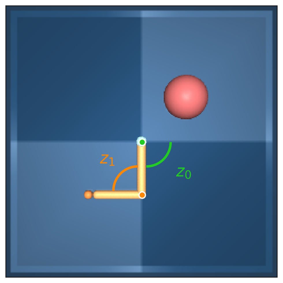
Environment and rendering.
The Reacher renderer is held fixed while the latent-state sampling process changes.
Encoder architecture.
A convolutional encoder maps pixels to the low-dimensional state representation.
Equation
Training.
Controlled Gaussian pairs and recorded-trajectory pairs define different training conditions.
Evaluation.
Recovery is measured against known joint coordinates, with planning evaluated separately.
Latent distributions.
The recorded trajectories need not have the independent Gaussian marginals of the controlled condition.
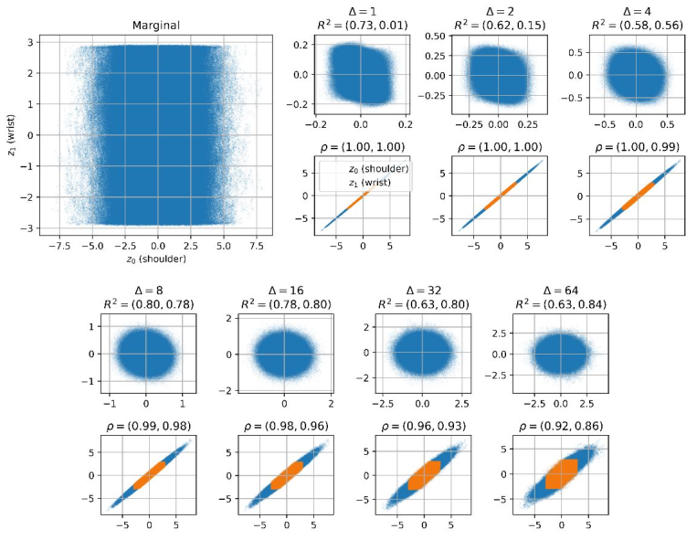
Gaussianity and autocorrelation jointly determine identifiability.
Both marginal shape and per-coordinate temporal correlation can affect recovery; this experiment changes multiple assumptions.
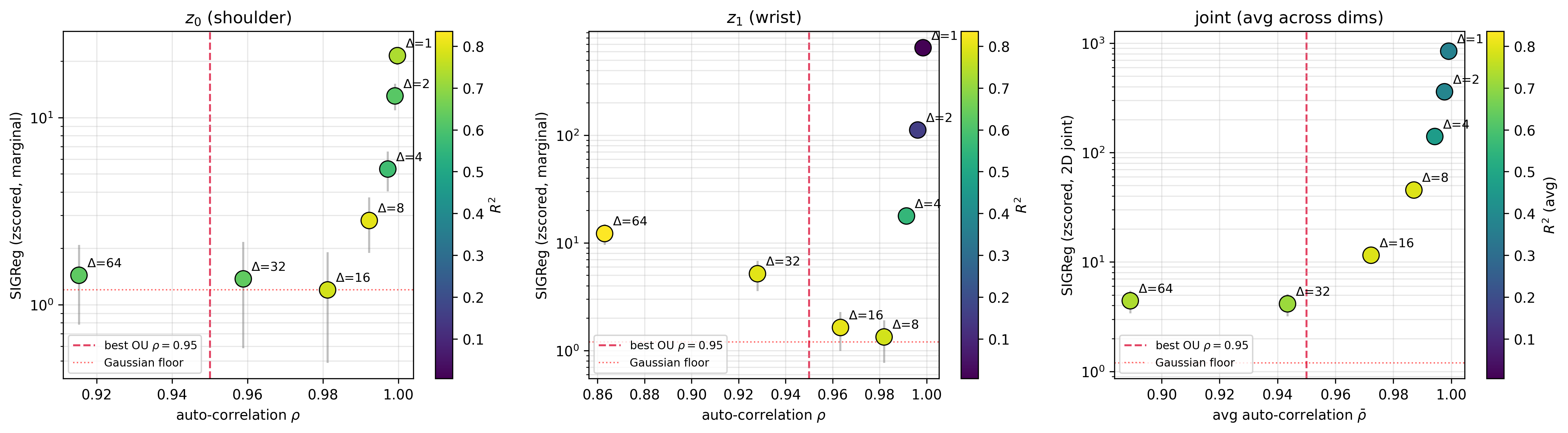
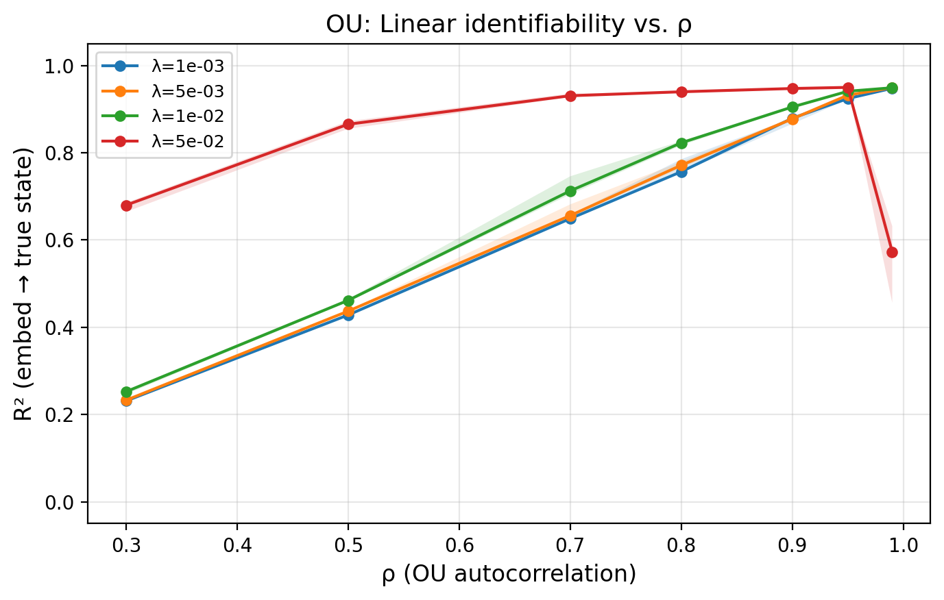
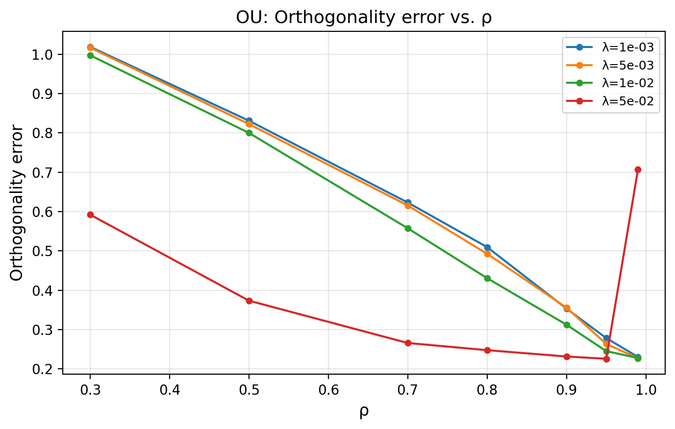
Additional results on OU and Trajectory conditions.
Additional plots expose the differences between controlled and policy-generated sampling.
H.12 Planning Experiment
Setup.
The planning test compares straight latent paths with the corresponding paths in known true-state coordinates.
Metric.
The reported control cost quantifies deviation from the particular goal-reaching optimum.
Interpretation.
Better linear recovery aligns the planning geometry in this task without establishing a universal controller ranking.
H.13 Misspecified Latent Dimension
Setup.
The encoder output dimension is deliberately set below, equal to or above the true latent dimension.
Results.
The reported subspace recovery and covariance participation ratio describe these controlled dimension-mismatch experiments.
| RealNVP, | Spiral, | ||||||
|---|---|---|---|---|---|---|---|
| PR | PR | ||||||
| 2 | 0.242 | 0.971 | 2.00 | 1 | 0.492 | 0.985 | 1.00 |
| 4 | 0.491 | 0.982 | 4.00 | 2 | 0.985 | 0.985 | 2.00 |
| 6 | 0.740 | 0.986 | 6.00 | 3 | 0.933 | 0.728 | 2.83 |
| 8 | 0.987 | 0.987 | 7.99 | 4 | 0.927 | 0.637 | 3.49 |
| 12 | 0.988 | 0.988 | 7.99 | 8 | 0.976 | 0.613 | 3.98 |
| 16 | 0.989 | 0.989 | 7.99 | 16 | 0.998 | 0.651 | 3.80 |
| 32 | 0.9490.06 | 0.988 | 7.190.75 | ||||
| 64 | 0.9770.02 | 0.986 | 7.710.39 | ||||
H.14 Predictors
Setup.
Linear and multilayer predictors are added to test an extension outside the simplest alignment formulation.
Results.
Recovery remains strong in the tested runs, but a general expressive-predictor guarantee is not established.
| Predictor | RealNVP () | Spiral () |
|---|---|---|
| None (Eq. 3) | 0.9890.001 | 0.9890.000 |
| Linear | 0.9870.001 | 0.9890.000 |
| MLP | 0.9880.001 | 0.9880.000 |
H.15 Training Dynamics
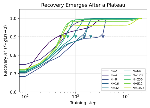
Recovery can appear after an initial optimization plateau. The population theorem does not specify when training must reach it.
| 2 | 4 | 8 | 16 | 32 | 64 | 128 | 256 | 512 | 1024 | 2048 | |
|---|---|---|---|---|---|---|---|---|---|---|---|
| median | 500 | 800 | 1500 | 1500 | 1500 | 1000 | 700 | 600 | 600 | 600 | 1000 |
| range | 200–600 | 600–1500 | 900–3500 | 700–2000 | 800–3000 | 700–3000 | 600–800 | 600 | 500–600 | 600 | 1000 |
H.16 ImageNet-X Linear Probes
Encoders.
The visual-encoder comparison records architectures, pretraining data and schedules.
Analysis space.
The chosen feature space determines which annotated factors the downstream probes can access.
Probes.
Linear probes measure labeled ImageNet-X factors without finetuning the visual encoder.
Results.
The results compare factor-readout accuracy under the stated protocols, not recovery of a known full natural-image generative state.
Gaussianity.
Empirical Gaussianity is approximate. Natural-image comparisons therefore remain empirical evidence beyond the controlled proof setup.
| IN-1k, matched | reference | controls | ||||||
| Factor | LeJEPA | DINO | iBOT | DINOv2 | DINOv3 | init | pixels | |
| class | 43500 | 0.865 | 0.666 | 0.741 | 0.856 | 0.813 | 0.620 | 0.585 |
| shape | 1276 | 0.737 | 0.590 | 0.661 | 0.709 | 0.657 | 0.552 | 0.575 |
| subcategory | 1118 | 0.720 | 0.604 | 0.648 | 0.682 | 0.614 | 0.554 | 0.502 |
| pattern | 11354 | 0.674 | 0.593 | 0.618 | 0.658 | 0.653 | 0.536 | 0.536 |
| smaller | 2738 | 0.651 | 0.618 | 0.663 | 0.627 | 0.692 | 0.529 | 0.538 |
| partial view | 1208 | 0.629 | 0.543 | 0.592 | 0.595 | 0.606 | 0.507 | 0.506 |
| color | 11642 | 0.616 | 0.571 | 0.580 | 0.599 | 0.606 | 0.544 | 0.526 |
| pose | 28404 | 0.605 | 0.559 | 0.583 | 0.598 | 0.589 | 0.530 | 0.516 |
| background | 27898 | 0.594 | 0.559 | 0.570 | 0.576 | 0.578 | 0.532 | 0.517 |
| darker | 230 | 0.809 | 0.714 | 0.751 | 0.643 | 0.620 | 0.700 | 0.520 |
| person blocking | 112 | 0.800 | 0.647 | 0.771 | 0.671 | 0.712 | 0.482 | 0.588 |
| texture | 542 | 0.664 | 0.619 | 0.643 | 0.698 | 0.625 | 0.548 | 0.521 |
| larger | 284 | 0.614 | 0.551 | 0.549 | 0.493 | 0.558 | 0.528 | 0.493 |
| style | 84 | 0.600 | 0.562 | 0.638 | 0.500 | 0.608 | 0.438 | 0.500 |
| brighter | 84 | 0.592 | 0.523 | 0.485 | 0.492 | 0.523 | 0.562 | 0.562 |
| multiple objects | 76 | 0.555 | 0.445 | 0.627 | 0.491 | 0.536 | 0.473 | 0.491 |
| object blocking | 152 | 0.552 | 0.565 | 0.435 | 0.574 | 0.513 | 0.491 | 0.474 |
| mean () | 0.677 | 0.589 | 0.628 | 0.656 | 0.645 | 0.545 | 0.533 | |
| mean (all 17) | 0.663 | 0.584 | 0.621 | 0.615 | 0.618 | 0.537 | 0.526 | |
| Linear | MLP | Gap | EP | PR | Excess kurtosis | |
|---|---|---|---|---|---|---|
| LeJEPA (projector) | 0.663 | 0.684 | 0.021 | 0.0049 | 0.91 | 0.39 |
| LeJEPA backbone (768-d) | – | – | – | 0.2534 | 0.08 | 0.38 |
| DINO | 0.584 | 0.617 | 0.033 | 0.5330 | 0.99 | 0.04 |
| iBOT | 0.621 | 0.632 | 0.011 | 0.6083 | 0.98 | 0.03 |
| DINOv2 | 0.615 | 0.645 | 0.030 | 0.4712 | 0.92 | 0.82 |
| DINOv3 | 0.618 | 0.643 | 0.025 | 0.0033 | 0.94 | 0.65 |
| init | 0.537 | 0.554 | 0.017 | 0.5311 | 0.06 | 1.18 |
| pixels | 0.526 | 0.540 | 0.014 | 0.5874 | 0.14 | 0.99 |
| sample | – | – | – | 0.00003 | 1.00 | 0.00 |