At a glance
Crys-JEPA learns a crystal embedding organized using formation-energy information, then uses it to rank generated structures for refinement. The goal is to improve the combination of validity, stability, uniqueness and novelty rather than merely generate plausible-looking structures. The system still uses force-field relaxation, known crystal references and selected DFT evaluations. It is a computational screening approach, not experimental confirmation of newly synthesized materials.
1 Introduction
A generator trained to imitate known crystals can favor familiar stable structures, while moving farther from that distribution can increase novelty and instability together. Crys-JEPA addresses this practical tradeoff by screening candidate structures and feeding promising ones back into a generator. The JEPA name describes its predictive embedding architecture; formation-energy differences provide additional supervised organization.
2 Preliminaries
A periodic crystal is represented by atom types, positions and a lattice. Thermodynamic stability compares its energy with mixtures of competing phases at the same composition. Energy above the convex hull therefore depends on a reference set; it is not simply the crystal’s absolute formation energy. Novelty is also relative to a specified structural matching criterion and reference database.
Equations 1–7
| (1) |
| (2) |
| (3) |
| (4) |
| (5) |
| (6) |
| (7) |
3 Stability and Novelty Trade-off: An Experimental Investigation
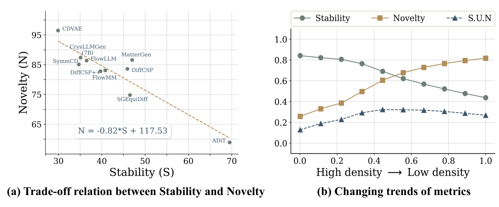
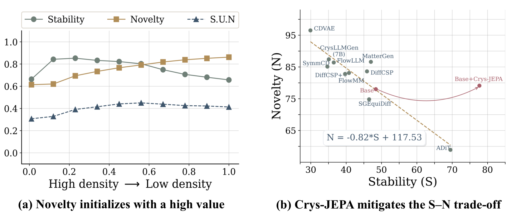
The authors compare generators and perturbations of known crystals using specified relaxation, reference data and stability thresholds. These experiments show a stability–novelty tension in the tested settings. They do not establish an immutable theorem that all unfamiliar crystals are unstable. Distance from a training set is measured by selected structural/compositional fingerprints and is itself a modeling choice.
Remark.
The stability–novelty trade-off is not a new observation, as it has also been reported in recent studies [37, 45, 48, 56]. In this section, we contribute new experimental evidence by systematically benchmarking current crystal generative models under a unified evaluation protocol. More specifically, beyond identifying the trade-off at the model level, our percentile-based analysis characterizes how stability, novelty, and S.U.N. evolve across different regions of the generated distribution. Our results show that samples farther from the empirical training distribution tend to exhibit higher novelty, but also a rapid deterioration in thermodynamic stability, thereby limiting the extent to which S.U.N. can be improved through likelihood maximization alone.
4 Mitigating the Stability–Novelty Trade-off
The proposed pipeline seeks promising candidates inside a large generated pool, ranks them with an energy-aware embedding and refines the original generator on selected examples. The embedding model and the generative model have different jobs.
4.1 Crys-JEPA: Energy-aware Crystal Latent Space via JEPA
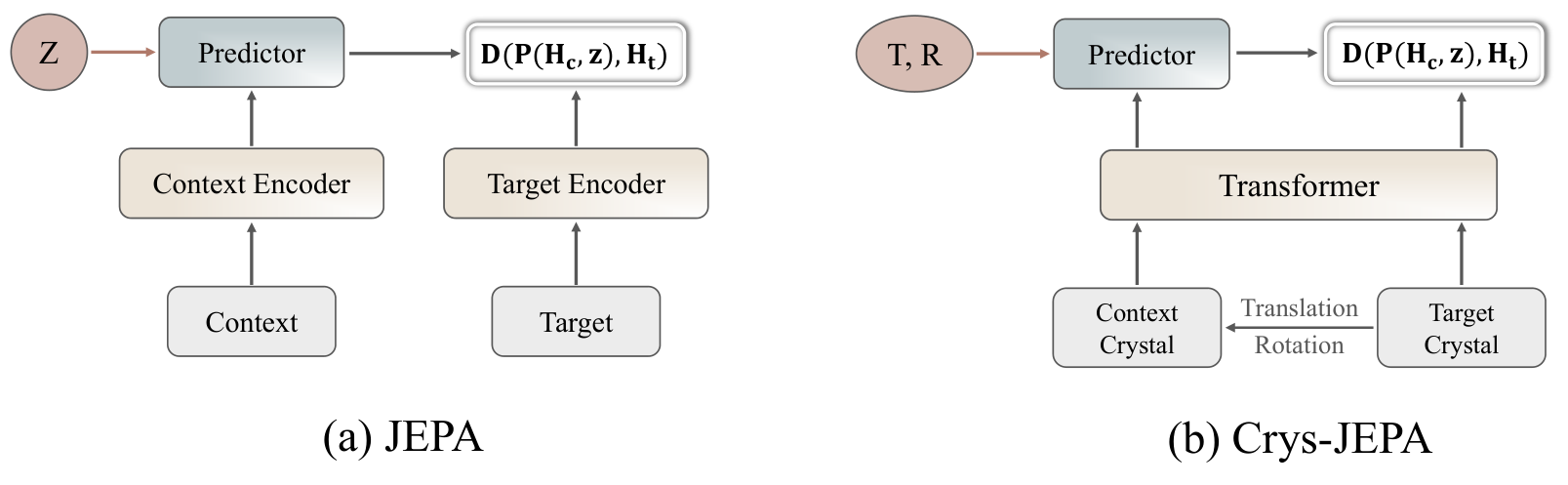
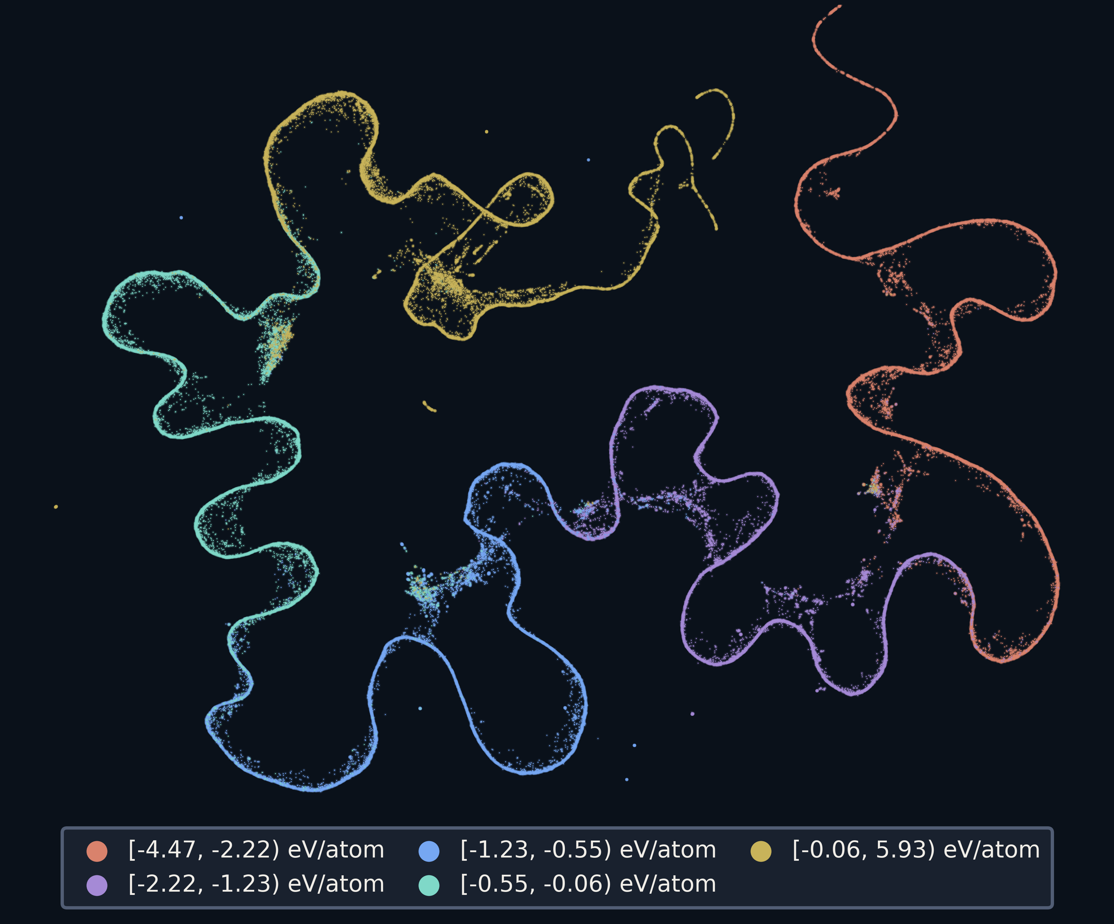
Rotation and translation supply crystal views that preserve formation energy. An encoder–predictor architecture is trained with an energy-aware contrastive objective: energy differences modulate how other crystals repel one another in embedding space. This uses energy information and negative examples, so it should not be described as pure label-free, negative-free masked JEPA. The aim is a useful stability-ranking surrogate rather than direct exact thermodynamic calculation.
Equations 8–10
| (8) |
| (9) |
| (10) |
4.2 Screening-and-Refinement Pipeline
Generated structures are first relaxed and filtered for validity, uniqueness and novelty. Each surviving candidate is compared with chemically relevant training crystals, including subsystem compositions, then ranked by the proposed embedding-distance heuristic. Selected candidates fine-tune the generator. The method reduces reliance on expensive screening, but does not eliminate force-field relaxation, reference structures or the need to validate selected structures.
Equation 11
| (11) |
Remark.
Conceptually, our proposed screening-and-refinement pipeline is similar to active learning, as both aim to identify the most informative samples for model training. Similar strategies have been successfully explored in materials science, notably in GNoME [32] and MatterSim [55]. However, traditional active learning pipelines in these works rely on computationally expensive, iterative DFT calculations to evaluate candidates and expand the training set. In contrast, our pipeline leverages Crys-JEPA as a surrogate screening signal, completely circumventing the need for further DFT annotation while maintaining effective refinement.
4.3 Why Use Embedding-Based Comparison for Stability Screening?
The embedding can retain structural information that a single energy scalar discards, making relative ranking useful. That is a motivation and an empirical comparison, not proof that every learned high-dimensional distance estimates stability better than an accurate energy calculation. The force-field and fingerprint baselines test concrete alternatives.
5 Numerical Experiments
Experiments apply screening and refinement to a diffusion-transformer generator and compare the resulting valid, stable, unique and novel fractions. Different evaluation backends and reference sets must remain explicit.
5.1 Crystal Generation on MP-20
On MP-20, refinement improves the combined metrics over the base generator and several baselines. The study supplements force-field scoring with DFT on selected 1000-sample comparisons, rather than applying that expensive calculation to every experiment. It also compares learned embeddings with fingerprints and alternative force fields. These comparisons test a whole pipeline, including sampling and refinement, not an isolated representation score alone.
| Model | S | N |
|
|
|
| ||||||||
| CDVAE† [51] | 29.91.2 | 96.50.6 | 27.01.3 | 22.81.1 | - | - | ||||||||
| DiffCSP [21] | 45.91.8 | 83.60.6 | 30.91.8 | 25.61.3 | - | - | ||||||||
| DiffCSP++ [22] | 39.72.0 | 82.81.0 | 23.81.3 | 20.31.2 | - | - | ||||||||
| FlowMM† [33] | 40.82.0 | 83.11.1 | 25.31.6 | 21.01.3 | - | - | ||||||||
| FlowLLM† [43] | 36.51.5 | 86.41.5 | 25.10.6 | 21.30.8 | - | - | ||||||||
| SymmCD† [28] | 34.71.4 | 85.11.5 | 19.00.9 | 15.70.8 | - | - | ||||||||
| ADiT [23] | 69.51.1 | 58.90.9 | 30.30.8 | 27.21.3 | - | - | ||||||||
| CrysLLMGen (7B)† [24] | 35.11.9 | 87.41.1 | 22.90.9 | 20.40.9 | - | - | ||||||||
| SGEquiDiff [8] | 46.51.9 | 74.81.2 | 23.50.9 | 20.01.0 | - | - | ||||||||
| MatterGen [57] | 47.01.1 | 86.61.0 | 34.61.2 | 29.20.9 | 30.8 | 26.4 | ||||||||
| Base model | 48.41.4 | 78.01.6 | 27.81.1 | 23.31.3 | - | - | ||||||||
| w/ Crys-JEPA | 76.61.1 | 83.31.1 | 45.21.4 | 44.91.4 | 48.1 | 47.9 |
| % | V | S | N | S.U.N | V.S.U.N |
|
| ||||
| Base model | 82.11.5 | 48.41.4 | 78.01.6 | 27.81.1 | 23.31.3 | - | 27,136 | ||||
| w/ Fingerprints | 94.11.0 | 53.11.4 | 72.91.2 | 22.90.7 | 21.90.7 | 1651.69 | - | ||||
| w/ CHGNet [11] | 96.80.3 | 74.71.3 | 77.40.6 | 39.80.9 | 38.20.7 | 339.49 | 1,580,395 | ||||
| w/ eSEN-30M-MP [14] | 95.80.3 | 77.21.0 | 80.20.9 | 44.00.8 | 41.01.1 | 843.53 | 1,580,395 | ||||
| w/ Crys-JEPA | 99.00.3 | 76.61.1 | 83.31.1 | 45.21.4 | 44.91.4 | 48.87 | 839,568 |
5.2 Crystal Generation base on Alex-MP-20
The larger Alex-MP-20 setting tests transfer of the pipeline under another dataset and reference correction scheme. The reported relative gain in the combined DFT metric is specific to that setup. It should not be turned into a universal gain in experimental discovery yield.
6 Conclusion
Crys-JEPA provides an energy-aware ranking tool inside a generative refinement pipeline. Its stability estimates remain surrogates. The authors explicitly require rigorous first-principles validation before treating candidates as definitive discoveries, and larger-scale modeling remains an open direction.
Acknowledgments and Disclosure of Funding
The source records funding and institutional support. These disclosures are attribution and should remain separate from the evidence for screening performance.
Appendix A Thermodynamic Stability Calculation
The derivation shows why elemental reference-energy terms cancel when comparing a crystal with composition-matched competing phases. Thus energy above hull can be computed consistently from total energies under the stated constraints. This does not remove dependence on the phase reference set or energy-calculation accuracy.
Equations 12a–16
| (12a) | ||||
| (12b) | ||||
| (13) | ||||
| (14) |
| (15) |
| (16) | ||||
Appendix B Model Details
Model details distinguish the denoising generator from the energy-aware crystal representation. Their architectures and training losses should not be conflated.
B.1 Diffusion-Based Generation
The generator learns to reverse a Gaussian noising process by predicting noise with a transformer. Sampling follows the learned reverse transitions. This is an ordinary diffusion generation component later improved through screening and fine-tuning; JEPA does not itself generate the crystal coordinates directly.
Equations 17–20
| (17) |
| (18) |
| (19) |
| (20) |
B.2 Transformer as Backbones
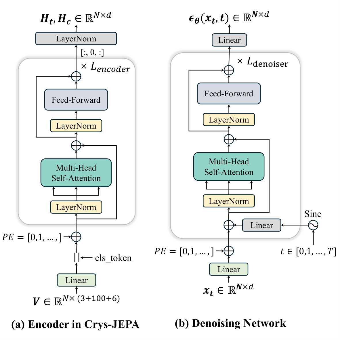
Both networks use transformer blocks, but the crystal encoder pools with a learned global token while the diffusion network is conditioned on a denoising timestep. The complete architectural diagram preserves those differences.
B.3 Hyperparameter Settings
The source specifies encoder depth, width, heads and the larger denoising network’s settings. These are the tested configurations rather than a claim that one architecture is optimal for every crystal dataset.
Appendix C More Experiments
The extra experiments probe sensitivity and what information is retained in the learned space. They help distinguish energy-aware screening from generic structural feature learning.
C.1 Hyper-Parameter Sensitivity Analysis
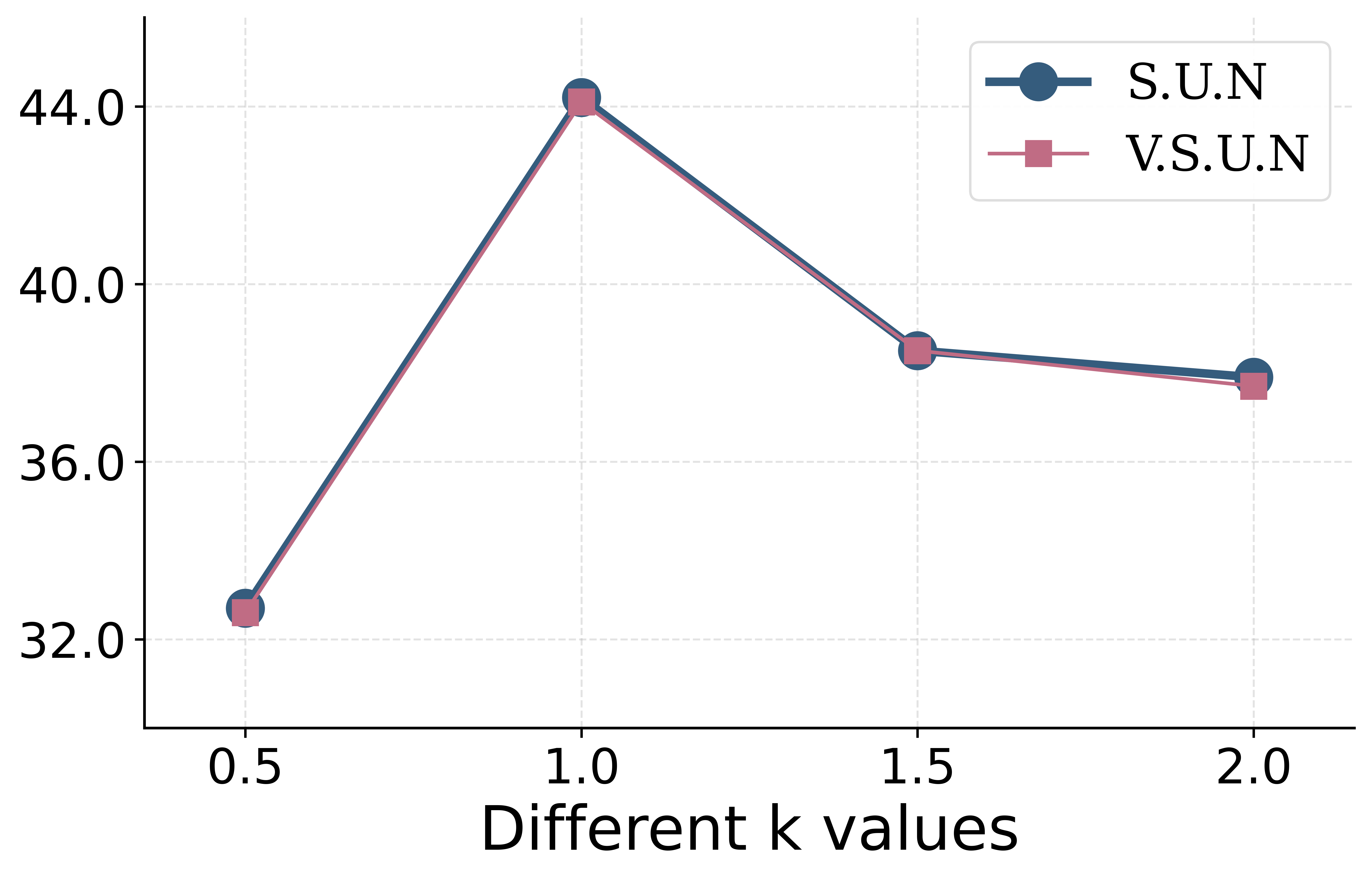
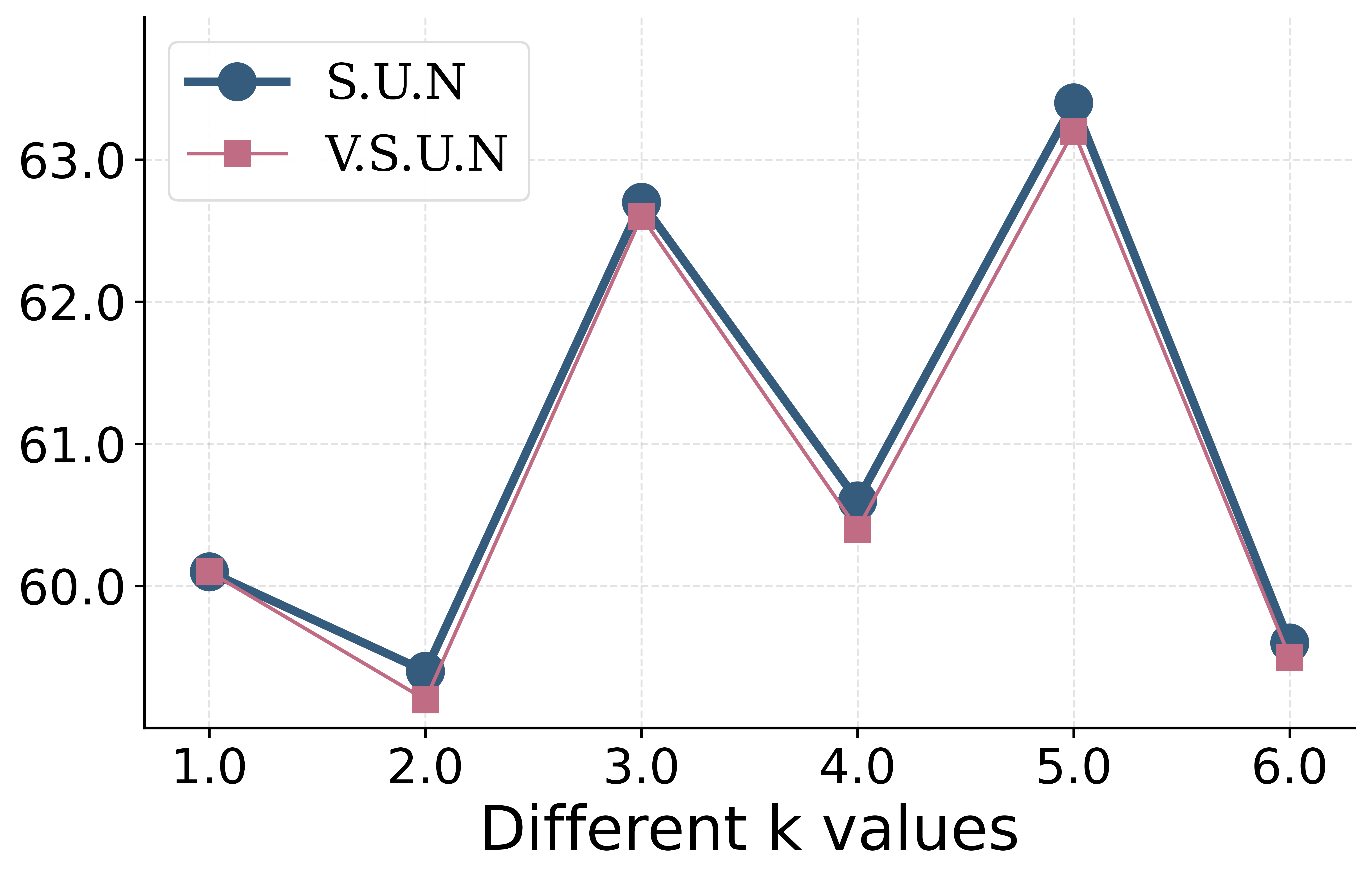
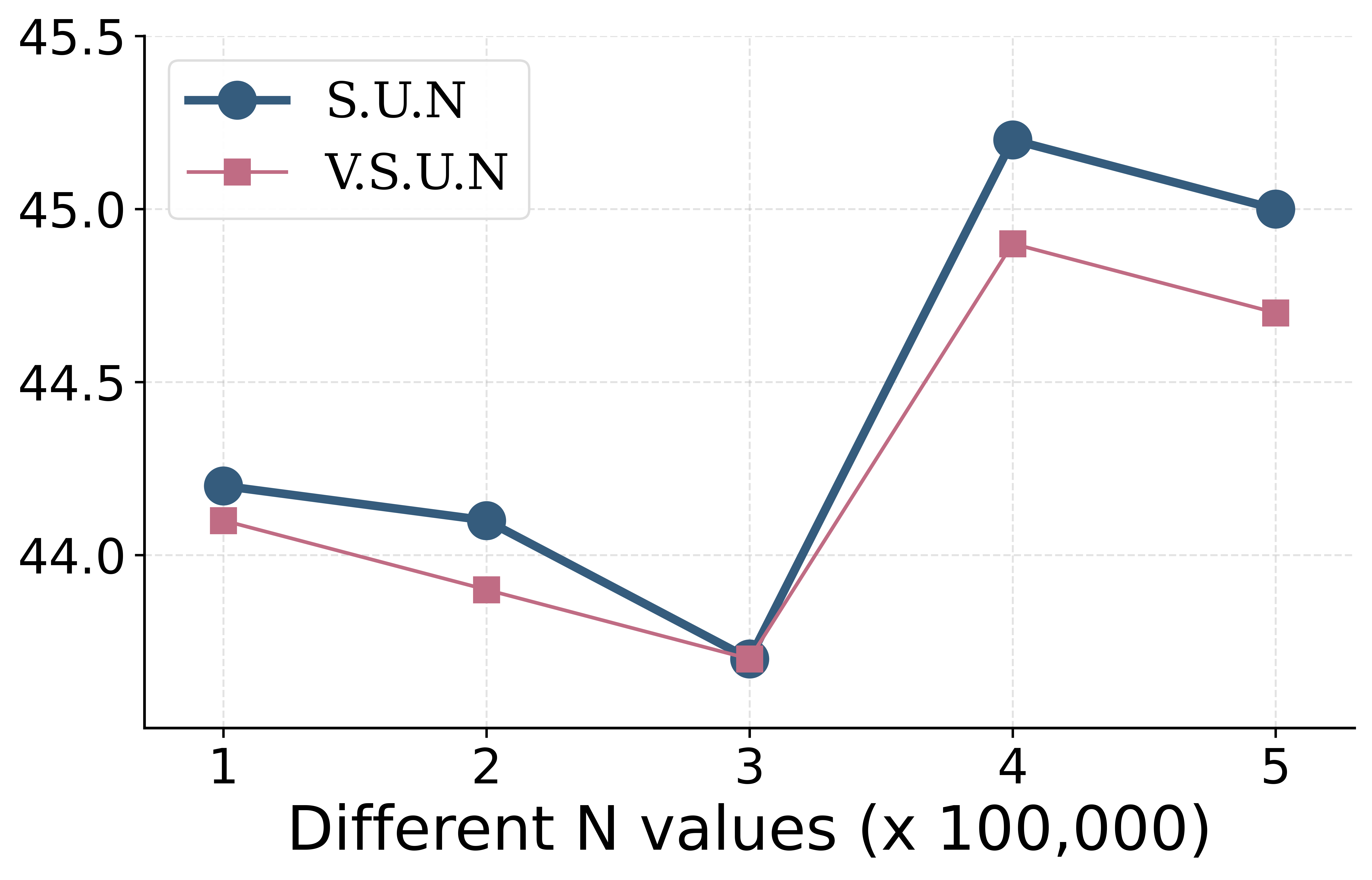
Keeping more generated candidates can expand diversity but also admit unstable examples. A larger initial pool can supply more useful candidates to screen. The resulting tradeoff means selection count and pool size are part of the method’s cost and quality, not inconsequential implementation constants.
C.2 Further Analysis of Crys-JEPA Representation
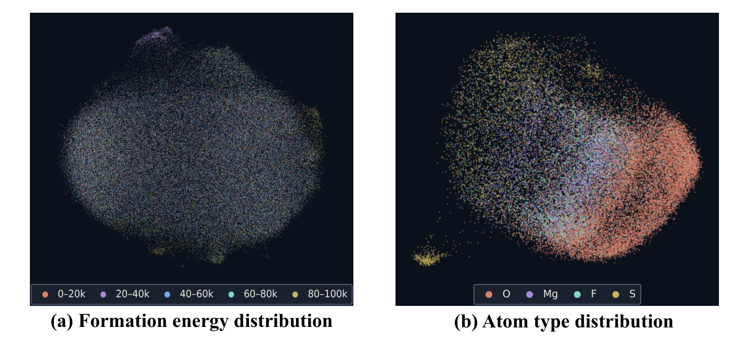
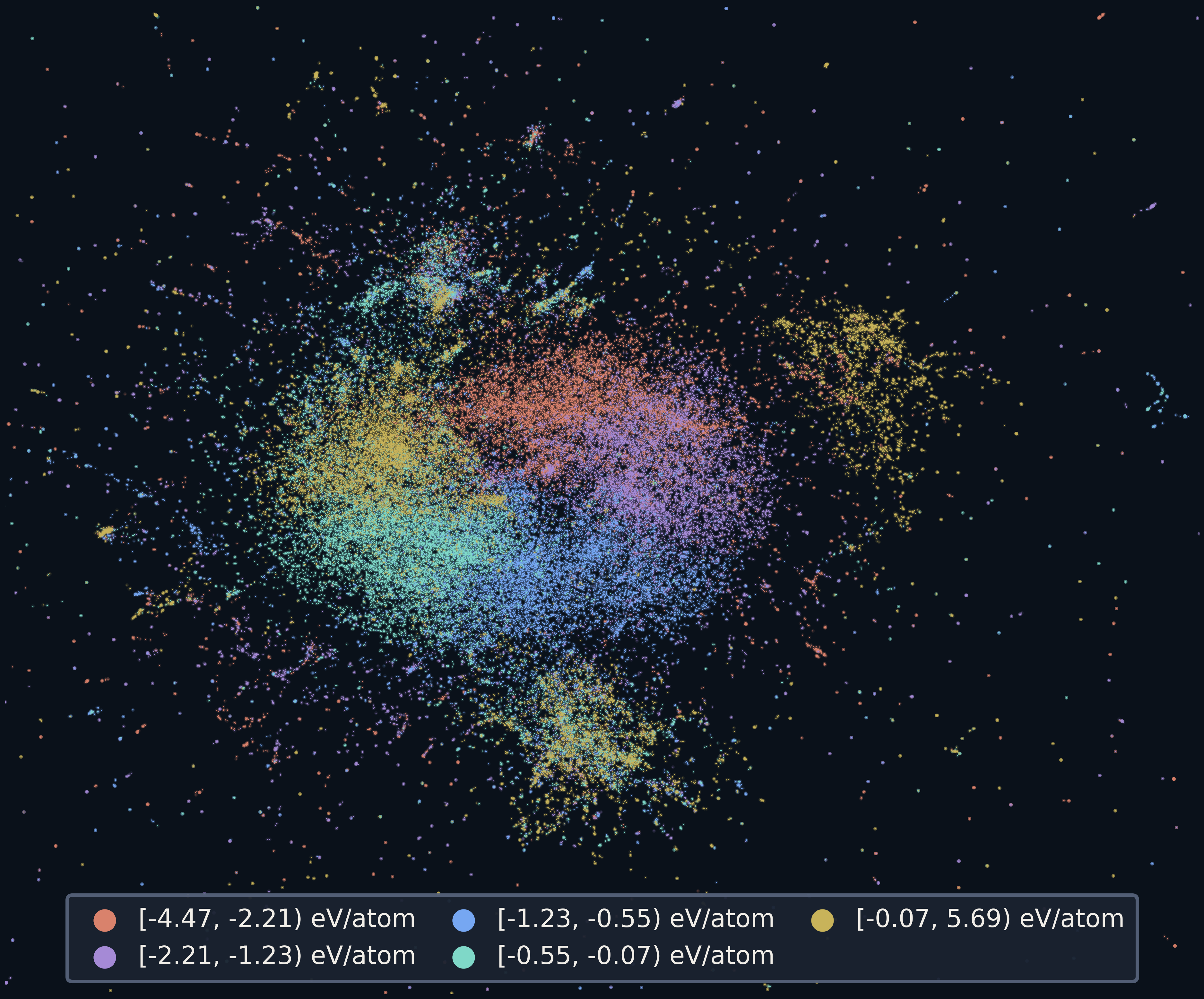
Removing energy-aware weighting changes the embedding’s organization, though some structural and elemental information remains. Additional plots show limitations of generic JEPA distances for stability screening. The SIGReg/MSE alternative studies collapse resistance, but avoiding collapse alone does not ensure that a representation orders crystals by the desired physical quantity.
Equations
Appendix D Experimental Details
The experimental details fix data splits, metrics, reference calculations, fingerprint distances and hardware so the combined discovery metrics can be interpreted reproducibly.
D.1 Datasets Descriptions
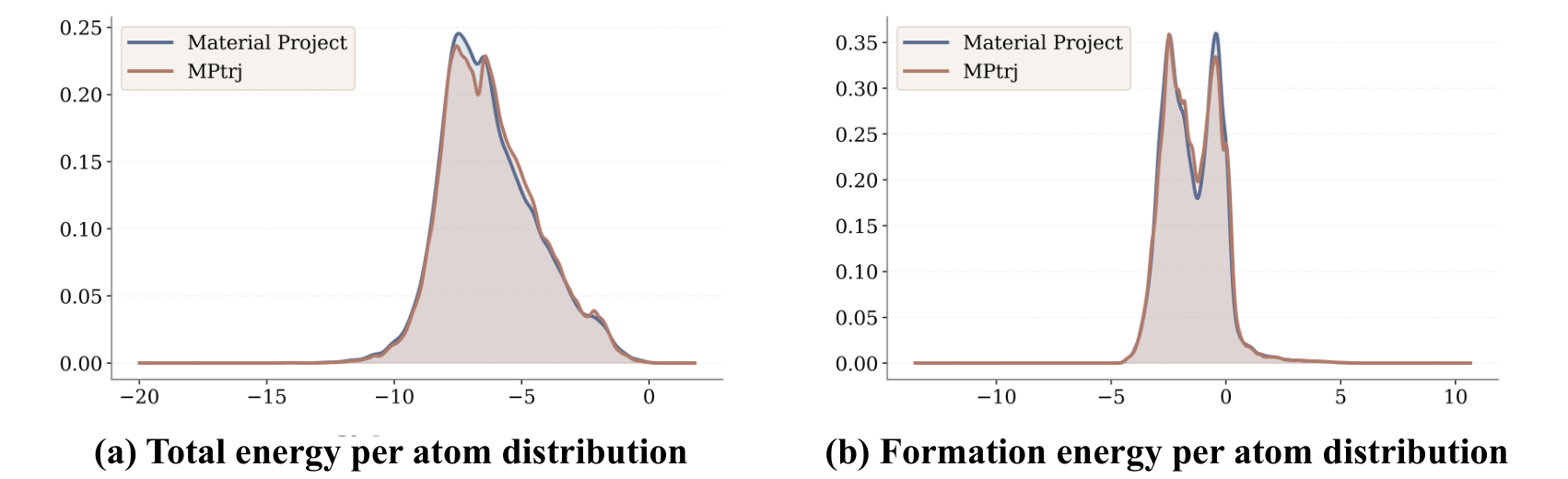
MP-20 and Alex-MP-20 differ substantially in size and curation, while both restrict unit-cell size. Train/validation/test splits and stability filtering affect which kinds of novelty are evaluated.
D.2 Evaluation Metric
Validity checks geometry and composition; stability uses energy above hull; uniqueness removes repeated samples; novelty checks against a reference set. The combined fractions depend on all those definitions. Passing these computational filters is not the same as successful laboratory synthesis.
Equations 21–23
| (21) |
| (22) |
| (23) |
D.3 Density Functional Theory Settings
The DFT workflow follows specified relaxation, functional and compatibility-correction settings. Failed initial relaxations may receive force-field pre-relaxation before another DFT attempt. Matching those choices matters when comparing energies with a reference database.
D.4 Distance based on Fingerprints
Fingerprint distances provide a baseline notion of structural and compositional similarity. Their feature design differs from the learned embedding’s energy-aware geometry.
D.4.1 CrystalNN and Magpie Fingerprints
CrystalNN summarizes local coordination environments; Magpie summarizes compositional element properties. They retain different information, and neither is itself a full thermodynamic stability calculation.
D.4.2 Definition of Distance
The distance combines normalized structural and compositional deviations from the training set. The normalization fixes how the two contributions are balanced; a numerical distance has meaning only with that definition.
D.5 Operating Environment
The reported operating environment documents the compute used for model and evaluation runs. It should be considered when assessing the pipeline’s practical screening cost.
Appendix E Related Work
Related work places the pipeline among scientific generative models, joint-embedding prediction and transformer representations. The architecture family alone does not identify the supervision used: this application explicitly incorporates formation-energy differences.