Overview
At a glance
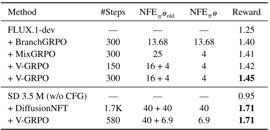
Variational GRPO replaces intractable image log-likelihoods with denoising-loss surrogates and stabilizes their optimization using shared noise/timesteps, stratified sampling, adaptive weighting and scenario-dependent update controls. It improves all four reported FLUX reward metrics and reaches a similar aggregate SD 3.5 Medium score with 580 rather than about 1,700 gradient updates. These are promising benchmark and computational-count results; the surrogate is not an exact likelihood ratio, and the stated speedups are not measured wall-clock guarantees.
1 Introduction
Text-to-image post-training needs rewards to influence a multi-step denoiser whose final-image likelihood is generally unavailable. Trajectory-based methods instead optimize tractable stochastic transitions, tying training to a particular rollout formulation. V-GRPO treats the whole generated image as one action and reuses an objective related to denoising pretraining.
The practical claim is that this simpler surrogate can work well when its stochastic variation and update size are controlled. It can roll out with a higher-order deterministic sampler without differentiating or assigning policy ratios to every transition. This edition covers all 14 pages of v1, dated 25 April 2026, with eight figures including all six ablation panels, six tables, Algorithm 1, 17 numbered equations and 47 references.
2 Related Work
Offline reward-weighted regression and direct preference optimization use fixed preference data, while online approaches refresh outputs from the current model. MixGRPO and BranchGRPO improve trajectory-based optimization with specialized sampling. Earlier denoising-loss surrogates performed poorly on visual generation; this work revisits their stability rather than introducing an exact tractable image likelihood.
DiffusionNFT also uses pretraining-style objectives but contrasts policies rather than using the same GRPO surrogate. The comparisons are with particular reported implementations and settings. The paper’s broad superiority language is stronger than what two model families and these reward benchmarks establish.
3 Preliminaries
3.1 Denoising Generative Models
A forward process mixes clean data with noise through schedule coefficients. The network regresses a chosen target, such as clean data, noise or velocity, using timestep-dependent weighting. Reverse sampling combines the current state, network output and optional stochastic noise; setting the stochastic term to zero yields an ODE-style update.
Compatible parameterizations can be related under a fixed forward process, motivating reuse of denoising losses across diffusion and flow models. This does not mean arbitrary trained networks, discretizations or weighting choices define identical final-image distributions. The experiments use rectified-flow models.
Equations 1–4
| (1) |
| (2) |
| (3) |
| (4) |
3.2 Group Relative Policy Optimization
GRPO normalizes each reward by the mean and standard deviation of outputs for the same prompt, avoiding a learned value critic. A PPO-style clipped objective limits the incentive for large likelihood-ratio changes. V-GRPO applies that template to an image-level surrogate rather than averaging transition-level ratios.
The printed normalization omits a zero-variance safeguard, relevant when all outputs receive the same coarse reward; implementation handling is not specified here. The method’s ratio approximation remains distinct from the exact ratio in the introductory GRPO formulation.
Equations 5–6
| (5) |
| (6) | ||||
Original selectable algorithm
4 Approach
4.1 Overview
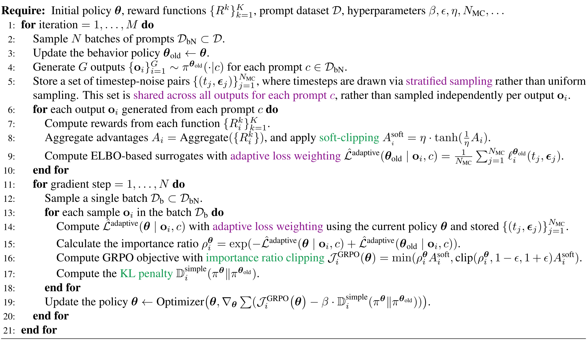
For each generated image, the algorithm estimates a negative denoising loss using a small number of sampled timestep/noise pairs. The exponential difference between current and behavior-policy losses becomes the GRPO ratio surrogate. Stored pairs are reused for the old and new evaluations, reducing irrelevant randomness and separating optimization from the rollout sampler.
Algorithm 1 refreshes the behavior policy, generates groups, computes rewards and advantages, stores old surrogate values, then updates the current policy over batches. Clipping and the old-policy penalty are enabled selectively. Exponentiating a noisy loss estimate does not make an unbiased likelihood-ratio estimate; nor does replacing two log-likelihoods with lower-bound-related objectives generally cancel their variational gaps.
Equations 7–10
| (7) | ||||
| (8) | ||||
| (9) |
| (10) |
4.2 Motivation
Variational diffusion connects log-likelihood lower bounds with noise-prediction error weighted by log-SNR change. Reparameterization and additional weights connect this to common pretraining objectives, providing a useful training surrogate.
The motivation establishes a relationship to variational learning, not equality between every weighted or adaptively normalized loss and the final-image log-likelihood. No theorem here bounds the error of the resulting importance ratios or guarantees policy-gradient improvement for the practical objective. Empirical stabilization is the main evidence.
Equations 11–13
| (11) |
| (12) |
| (13) |
4.3 Diagnosing Instability
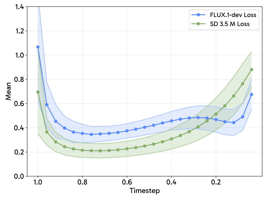
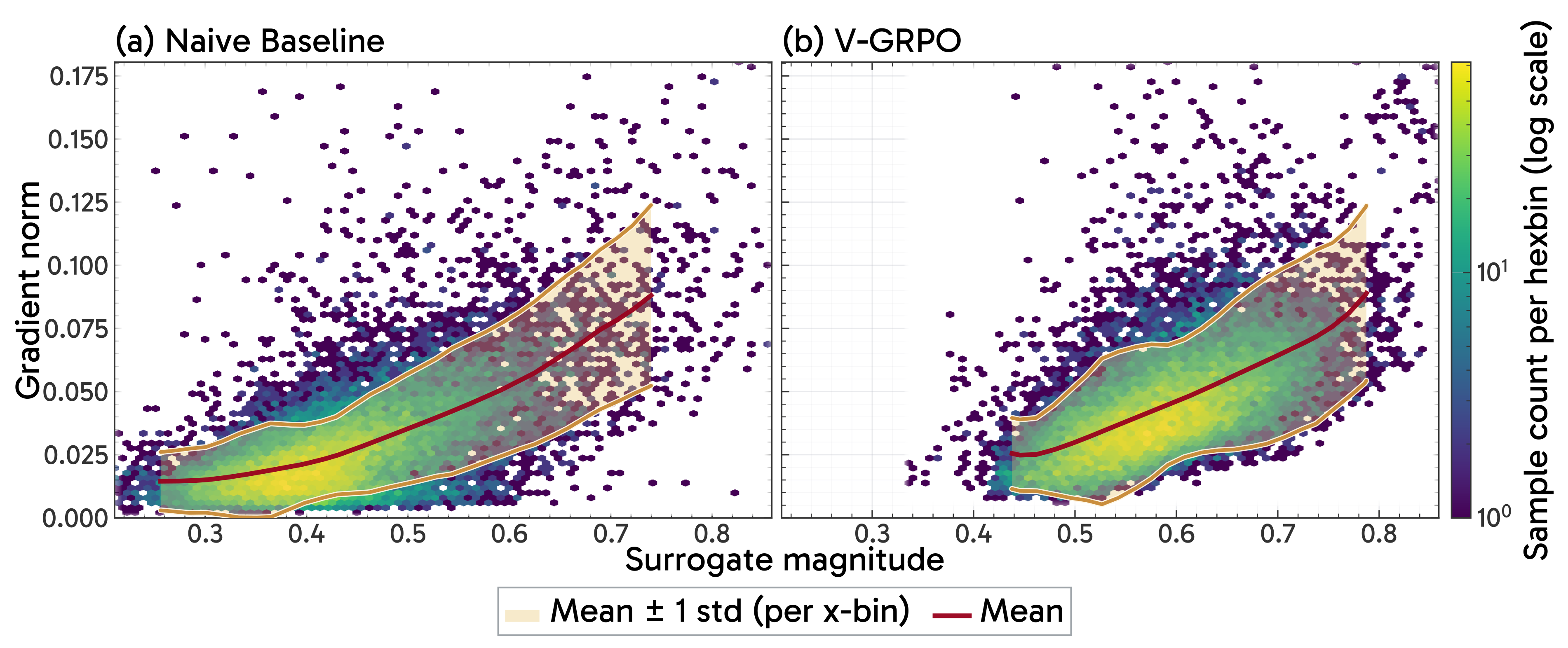
Loss magnitude varies strongly across timesteps in 400 sampled images. A separate analysis of roughly 20,000 FLUX samples associates larger surrogate values with larger gradient norms. Those gradients are measured through the ratio before advantage scaling or clipping, so they do not directly measure the complete training update.
The authors hypothesize that stochastic surrogate scale can overwhelm reward information. These correlations motivate the following controls; the ablations, rather than the correlations alone, test their training consequences.
4.4 Reducing Surrogate Variance
Motivated by the preceding analysis, we identify three surrogate variance reduction techniques that prove effective.
Group-shared timestep-noise pairs.
All images in a prompt group use the same sampled timestep/noise pairs. This common-randomness construction removes a source of within-group differences unrelated to reward and makes output comparisons less noisy. It does not eliminate all image-dependent surrogate error or independently establish an exact likelihood ranking.
Stratified timestep sampling.
The schedule is divided into as many equal-length strata as there are Monte Carlo pairs, with one timestep drawn per stratum. Each estimate therefore covers the schedule instead of accidentally concentrating in one region. This controls timestep sampling variability; the exact schedule and finite-sample estimator still affect the objective.
Adaptive loss weighting.
Predictions are converted to clean-image coordinates, then squared error is divided by the stop-gradient mean absolute error. For rectified flow, clean-image error scales with timestep, changing the effective emphasis across noise levels. Normalization approximately equalizes gradient scales across samples.
The denominator depends on the current prediction but is held constant during differentiation. This is a practical adaptive surrogate, not a fixed exact likelihood objective. The displayed denominator has no explicit numerical floor, so zero-residual handling is an implementation detail not documented by the formula.
Equation 14
| (14) |
Together the controls reduce surrogate coefficient of variation from 0.230 to 0.128 and mean within-group variation from 0.170 to 0.038. The quadratic fit between surrogate magnitude and gradient norm has R² 0.406 before and 0.328 after. The latter is a measure of association, not itself a variance or a causal sensitivity coefficient.
4.5 Controlling Gradient Steps
Variance reduction is applied throughout, while update regularization depends on the training regime. The tested choices are clipped ratios, a penalty toward the immediately preceding behavior policy, and smooth advantage bounding. No single combination is best for every reward and update schedule.
Importance ratio clipping.
Ratio clipping is the default for batches updated after the policy has moved away from the rollout policy. It limits the surrogate incentive for sufficiently large changes; it is not a hard constraint on the complete learned distribution or every parameter update. FLUX’s tested clipping ranges are small and depend on rollout length.
KL penalty.
The behavior-policy penalty discourages changes in denoised predictions on stored noisy samples. This supplies an inexpensive consistency regularizer without necessarily keeping a separate long-lived reference model. Its practical squared-prediction form should not be read as a directly measured KL between final-image distributions.
The text says only old scalar losses need be cached, but Equation 16 additionally requires old predictions or an equivalent recomputation path. That cache detail is omitted; the paper alone does not establish an implementation defect. The penalty helps retain earlier GenEval capability during OCR training but does not prevent FLUX loss spikes by itself.
Equations 15–16
| (15) | ||||
| (16) |
Original selectable table
| Method | HPS-v2.1 | PickScore | ImageReward | UnifiedReward | ||
| FLUX.1-dev | — | — | 0.313 | 0.227 | 1.088 | 3.370 |
| + DanceGRPO | 25 | 4 | 0.334 | 0.225 | 1.335 | 3.374 |
| 25 | 4∗ | 0.333 | 0.229 | 1.235 | 3.325 | |
| 25 | 14 | 0.356 | 0.233 | 1.436 | 3.397 | |
| + BranchGRPO-WidPru | 13.68 | 8.625 | 0.364 | 0.231 | 1.609 | 3.383 |
| + BranchGRPO-DepPru | 13.68 | 8.625 | 0.369 | 0.235 | 1.625 | 3.404 |
| + BranchGRPO-Mix | 13.68 | 4.25 | 0.363 | 0.230 | 1.598 | 3.384 |
| + BranchGRPO | 13.68 | 13.68 | 0.363 | 0.229 | 1.603 | 3.386 |
| + MixGRPO-Flash | 8 | 4∗ | 0.357 | 0.232 | 1.624 | 3.402 |
| 16 | 4 | 0.358 | 0.236 | 1.528 | 3.407 | |
| + MixGRPO | 25 | 4 | 0.367 | 0.237 | 1.629 | 3.418 |
| + V-GRPO | 16 + 4 | 4 | 0.372 | 0.241 | 1.731 | 3.437 |
| 25 + 4 | 4 | 0.372 | 0.241 | 1.749 | 3.436 |
Advantage soft-clipping.
Advantages are transformed by η tanh(A/η), preserving small values while smoothly bounding extremes. In a single-update iteration the current and old policies initially coincide: ratios are one and ratio clipping is locally inactive, while the prediction-consistency penalty has zero gradient. The policy gradient itself can still be nonzero, so advantage bounding remains useful.
It stabilizes the tested on-policy SD preference stage and shorter FLUX rollouts, but can suppress useful signal for coarse GenEval rewards. Its benefit is therefore conditional on reward and update structure.
Equation 17
| (17) |
The final recipe uses all three variance controls, ratio clipping in ordinary multi-update settings, a behavior-policy penalty when retaining prior skills matters, and advantage soft-clipping for on-policy or short-rollout cases. Algorithm 1 shows all options together; the experiment configurations specify which are actually enabled.
5 Experiments
5.1 Experiment Setup
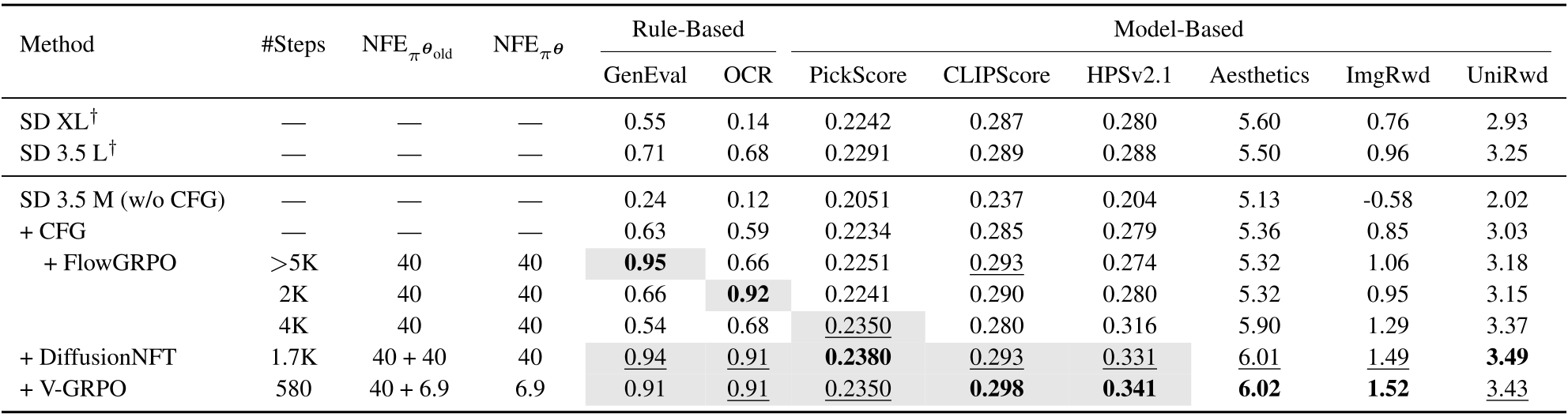
Original selectable table
| Method | #Steps | Rule-Based | Model-Based | ||||||||
| GenEval | OCR | PickScore | CLIPScore | HPSv2.1 | Aesthetics | ImgRwd | UniRwd | ||||
| SD XL† | — | — | — | 0.55 | 0.14 | 0.2242 | 0.287 | 0.280 | 5.60 | 0.76 | 2.93 |
| SD 3.5 L† | — | — | — | 0.71 | 0.68 | 0.2291 | 0.289 | 0.288 | 5.50 | 0.96 | 3.25 |
| SD 3.5 M (w/o CFG) | — | — | — | 0.24 | 0.12 | 0.2051 | 0.237 | 0.204 | 5.13 | -0.58 | 2.02 |
| + CFG | — | — | — | 0.63 | 0.59 | 0.2234 | 0.285 | 0.279 | 5.36 | 0.85 | 3.03 |
| + FlowGRPO | 5K | 40 | 40 | 0.95 | 0.66 | 0.2251 | 0.293 | 0.274 | 5.32 | 1.06 | 3.18 |
| 2K | 40 | 40 | 0.66 | 0.92 | 0.2241 | 0.290 | 0.280 | 5.32 | 0.95 | 3.15 | |
| 4K | 40 | 40 | 0.54 | 0.68 | 0.2350 | 0.280 | 0.316 | 5.90 | 1.29 | 3.37 | |
| + DiffusionNFT | 1.7K | 40 + 40 | 40 | 0.94 | 0.91 | 0.2380 | 0.293 | 0.331 | 6.01 | 1.49 | 3.49 |
| + V-GRPO | 580 | 40 + 6.9 | 6.9 | 0.91 | 0.91 | 0.2350 | 0.298 | 0.341 | 6.02 | 1.52 | 3.43 |
Base models.
FLUX.1-dev is already guidance-distilled and runs without explicit classifier-free guidance. SD 3.5 Medium is normally guidance-dependent, but the main multi-stage experiments disable CFG during both training and evaluation. Reward training improves that unguided model; this is tested on the named models rather than a general guarantee that RL always replaces CFG.
Reward functions.
Rule-based rewards use GenEval for compositional alignment and OCR for text rendering. Learned rewards include HPSv2.1, PickScore, CLIPScore, ImageReward, UnifiedReward and Aesthetics. These are benchmark proxies, not a new blinded human preference study; optimizing them can introduce reward-specific biases.
Prompt datasets.
FLUX uses HPDv2 prompts. SD’s GenEval and OCR stages use Flow-GRPO prompt sets; preference stages train on Pick-a-Pic and evaluate on DrawBench. Metric and prompt choices differ by stage, so evaluation should be read with the curriculum and in-domain shading in the tables.
Training and evaluation.
Rollouts use second-order DPM-Solver++, while evaluation returns to first-order Euler to match baselines. Extra old-policy evaluations are needed because rollout predictions cannot simply supply the chosen denoising-loss samples. Rollouts use BF16, but master weights, old/current surrogate calculations and backward passes use FP32.
NFE counts model evaluations; it is not a complete wall-clock or memory measurement. Baseline results are imported from their original papers. The source reports restricted hyperparameter tuning but no repeated-seed uncertainty or common-hardware timing study.
5.2 FLUX.1-dev Main Results
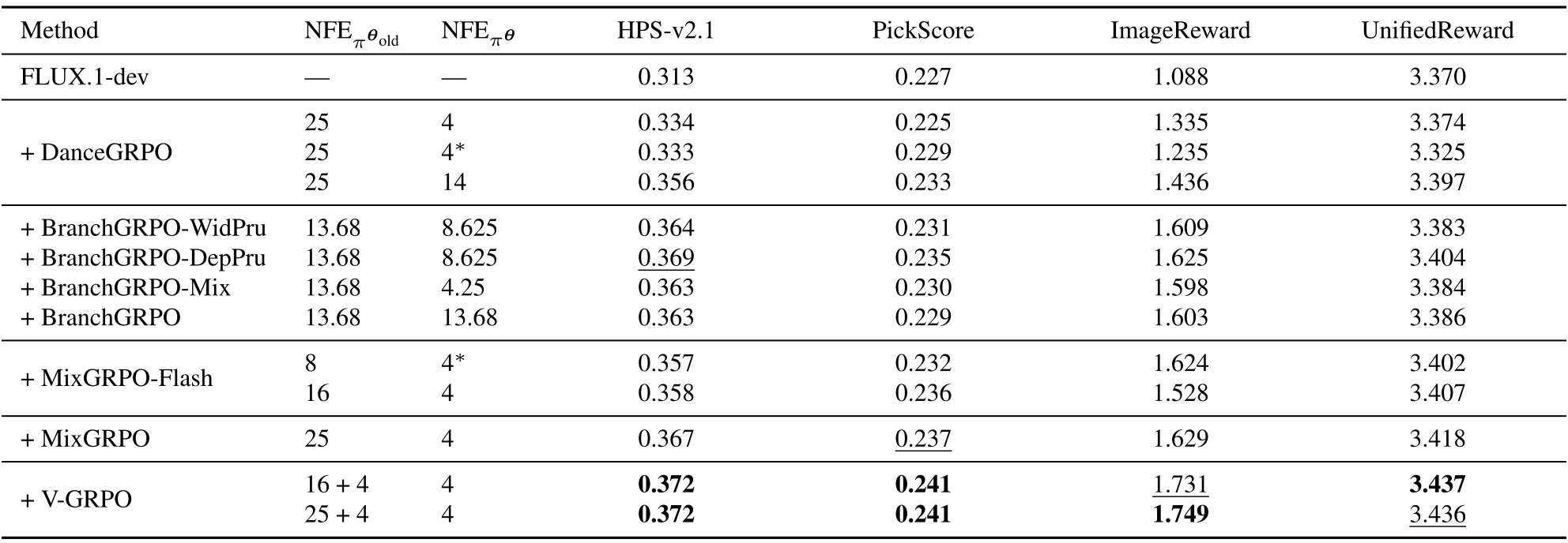
After 300 FLUX training iterations, the 16-step V-GRPO configuration scores HPSv2.1 0.372, PickScore 0.241, ImageReward 1.731 and UnifiedReward 3.437, above the listed baselines in all four columns. The 25-step configuration gives 0.372, 0.241, 1.749 and 3.436, so longer rollout improves one metric slightly while reducing another slightly.
The reported 2× comparison is 150 versus 300 iterations to a similar mean reward, with different evaluation counts. Each V-GRPO iteration has four gradient updates; the table’s “steps” for FLUX are iterations, unlike the SD gradient-update counts. Table 1 averages heterogeneous raw reward scales, so its scalar score can conceal per-metric tradeoffs.
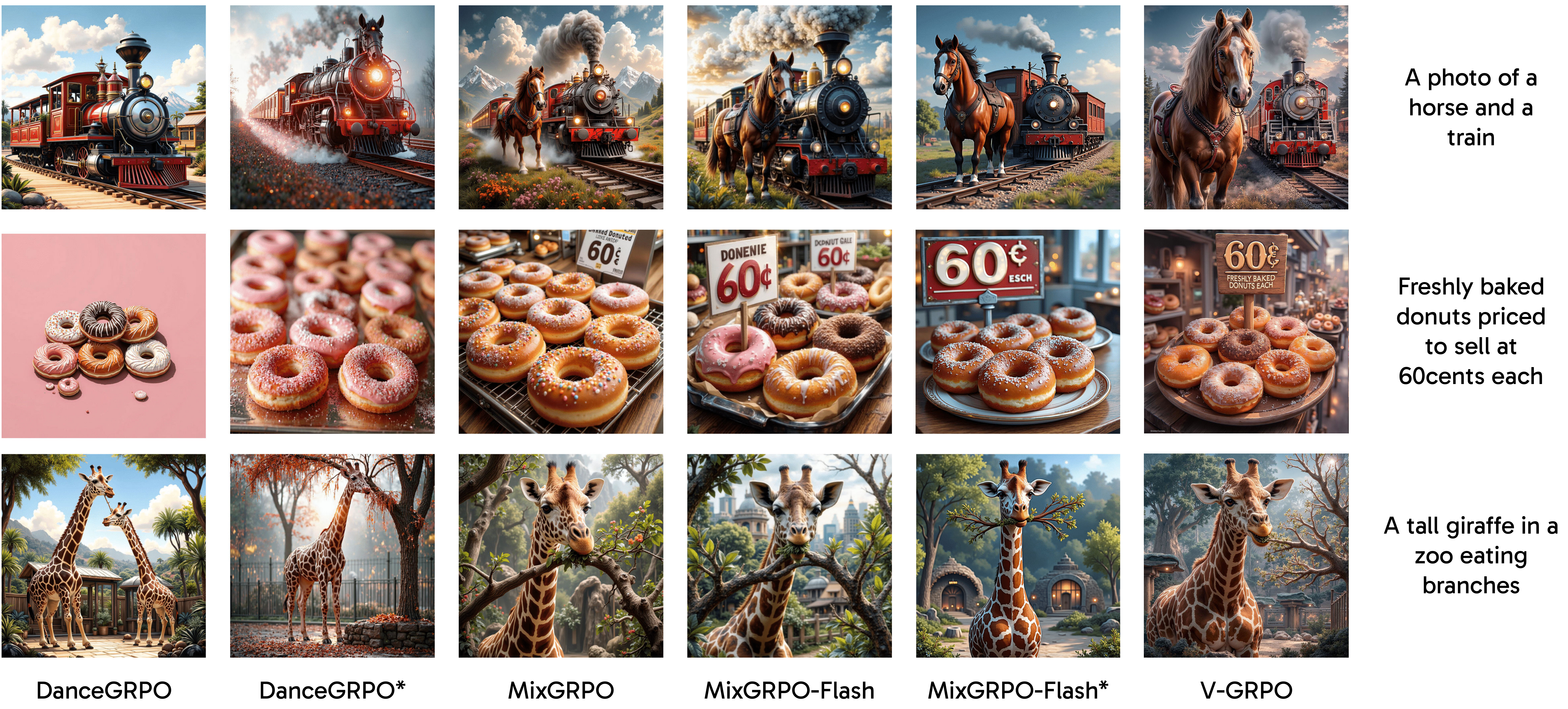
Evaluation mixes the trained model for the first 80% of denoising with the original base model for the rest, following MixGRPO. The result is therefore for this hybrid sampler, not an unmixed fine-tuned checkpoint. Selected examples demonstrate useful text and composition behavior, but do not quantify general world knowledge or human preference.
5.3 SD 3.5 M Main Results
The five-stage SD curriculum uses 580 gradient updates, versus roughly 1,700 for DiffusionNFT. It matches the rounded raw-score mean of 1.71, while trading metrics: GenEval is 0.91 versus 0.94, PickScore 0.2350 versus 0.2380 and UnifiedReward 3.43 versus 3.49; OCR ties at 0.91, while CLIPScore, HPSv2.1, Aesthetics and ImageReward are slightly higher.
Thus “matches performance” refers to a heterogeneous aggregate, not equivalence on each task. The comparison supports fewer updates and lower listed NFE; it does not establish a measured 3× time reduction. Main SD models evaluate at 512×512, while some reference models in Table 3 are marked as using 1024×1024.
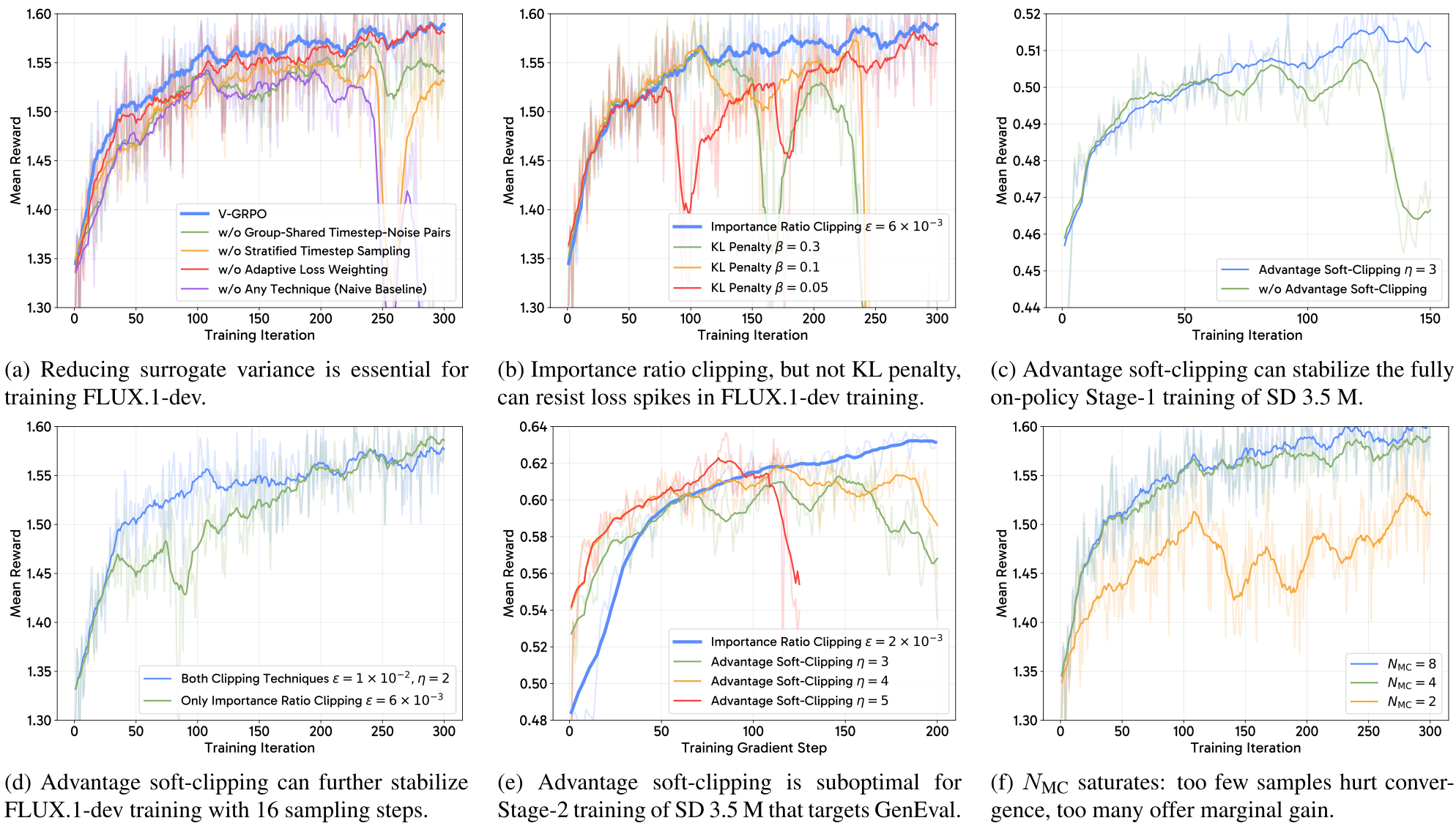
Original selectable panel captions
5.4 Ablation Studies
Reducing surrogate variance.
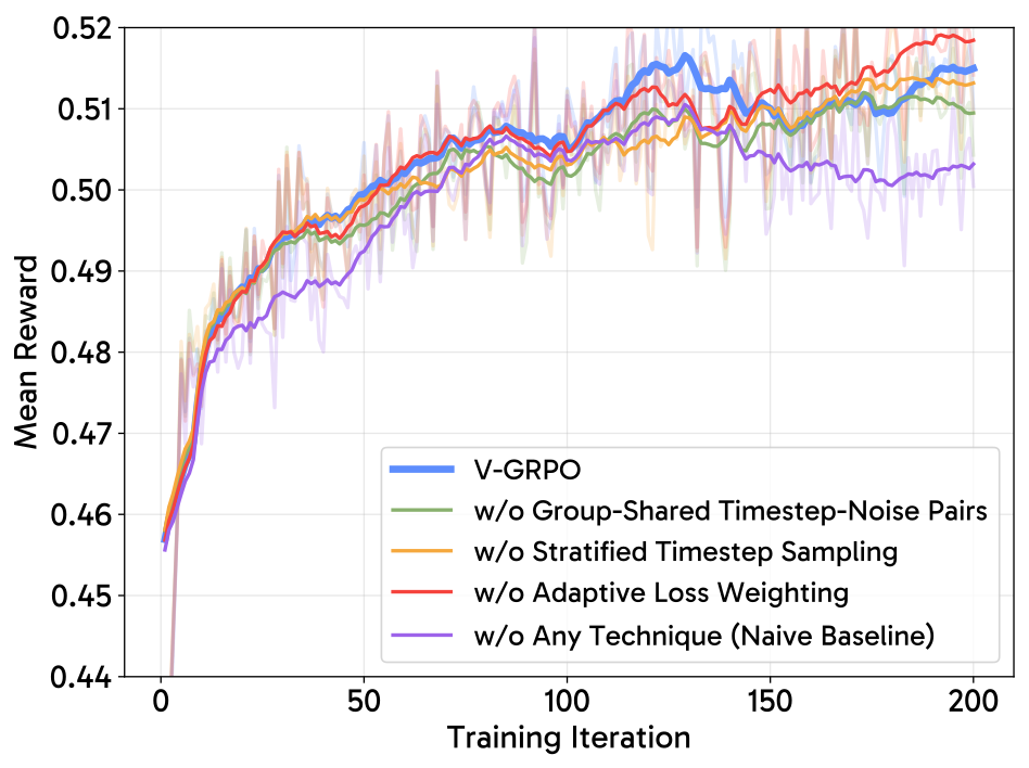
On FLUX, removing shared pairs or stratification destabilizes training; removing adaptive weighting causes a smaller performance loss. On SD preference training, no single component is critical in isolation, though removing all is worse. The effects depend on the base model and setup, rather than proving each component is always necessary.
Controlling gradient steps.
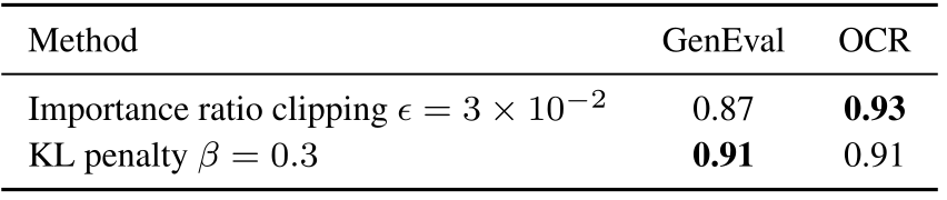
During the final SD OCR stage, a behavior-policy penalty preserves GenEval at 0.91 with OCR 0.91; ratio clipping gives GenEval 0.87 and OCR 0.93. This is retention versus specialization, not a uniform win. The prose cites a preceding GenEval value of 0.92, but Table 4 shows only the two final configurations.
FLUX still spikes under penalty-only updates. Soft-clipped advantages help SD’s single-update preference stage and 16-step FLUX rollout, yet underperform ratio clipping in the coarse-reward GenEval stage. All six Figure 4 panels are retained.
Effect of N MC .
On FLUX, two Monte Carlo pairs fail to converge well, four work substantially better, and eight add little. This is a tested saturation pattern rather than a universal optimum; SD uses ten pairs during several task-focused stages.
6 Conclusion
The study shows that a stabilized denoising-loss surrogate can be a strong, flexible online post-training method on these image benchmarks. Its value is practical compatibility with existing pretraining losses and decoupled sampling. Remaining limits include surrogate bias, reward gaming, model-specific tuning, limited uncertainty reporting and the lack of wall-clock or broader-domain evidence behind the strongest general claims.
Acknowledgments.
The authors credit feedback from Xinghan Li and partial computational support from Lambda; Serena Yeung-Levy is identified as a Chan Zuckerberg Biohub investigator.
Appendix A Additional Implementation Details
Our implementation adheres closely to the baseline methods, with deviations limited to the key techniques described in Sec. 4.4 and Sec. 4.5.
A.1 FLUX.1-dev Experiments
Main experiments.
FLUX averages the separately normalized advantages from four rewards. AdamW uses learning rate 10⁻⁵ and weight decay 10⁻⁴, with 300 iterations, four gradient updates per iteration, global batch size eight per update and group size twelve. There is no weight EMA. Four timestep/noise pairs are used throughout.
With 25 rollout steps, ratio clipping is 0.006. With 16 steps, it is 0.01 plus advantage bound two. Neither uses the old-policy penalty. Rollouts are 720×720; evaluation is 50 steps at 1024×1024, using the trained model for the first 40 steps and the base model for the final ten. The latter is explicitly intended to mitigate reward hacking.
Ablation studies.
The appendix gives 25 rollout steps as the default FLUX ablation setting, with main-experiment settings otherwise unchanged. Figure 4(d) explicitly studies 16 steps and is the stated exception. Ablation plots show training reward, not an independent held-out human assessment.
A.2 SD 3.5 M Experiments
Main experiments.
SD first averages rewards and then normalizes group advantages, unlike FLUX’s average of per-reward advantages. LoRA uses rank 32 and scale 64; AdamW uses learning rate 3×10⁻⁴ and weight decay 10⁻⁴. Global batch size is 48 per gradient step and group size 24. Optimizer state is reset between stages, and no EMA is kept.
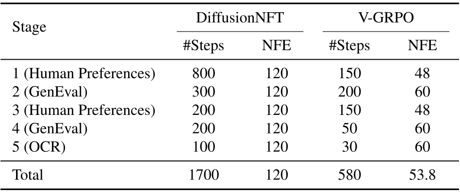
Stages 1 and 3 each use 150 single-update iterations on preference rewards, four Monte Carlo pairs and advantage bound three. Stage 2 adds GenEval for 100 two-update iterations with ten pairs and ratio bound 0.002. Stage 4 repeats this for 25 two-update iterations with ratio bound 0.004. Stage 5 replaces GenEval with OCR for 15 two-update iterations, ten pairs and penalty coefficient 0.3. The total is 440 iterations and 580 gradient updates.
Training and evaluation use 40 sampling steps at 512×512. The gradient-step-weighted mean pair count is about 6.9, and Table 5’s mean NFE is about 53.8 versus 120 for DiffusionNFT. Baseline stage counts are approximate because of early stopping. CLIPScore is called out-of-domain in one appendix sentence despite being used in the preference ensemble; that label is inconsistent with the stated curriculum.
Single-reward experiments.
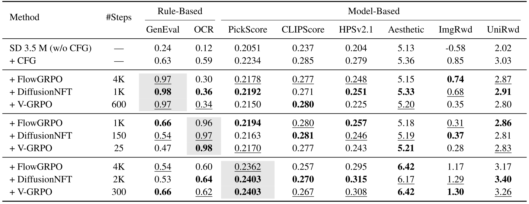
Single-reward GenEval training runs 300 two-update iterations, or 600 updates, using Stage 4 settings. OCR runs 25 single-update iterations with ten pairs and advantage bound four. PickScore runs 300 single-update iterations with four pairs and advantage bound three.
For OCR-trained models, CFG is re-enabled when evaluating non-OCR rewards, following the baseline protocol; the blanket no-CFG description has this explicit exception. GenEval reaches 0.97 versus DiffusionNFT’s 0.98; OCR reaches 0.98 versus 0.97; PickScore ties at 0.2403. Other metrics vary, so fast optimization of a target reward is not uniform preservation of all capabilities.
Ablation studies.
SD ablations otherwise use the corresponding main-stage configuration. Figure 5’s horizontal axis extends to 200 iterations although the main preference stages are described as 150; the source does not detail that duration difference. It still shows that removing all controls is worse while individual removals have modest effects.
Appendix B Additional Results
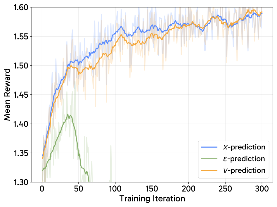
Additional examples retain every model row, prompt and image panel. Figure 6 compares adaptive weighting under different prediction coordinates: noise prediction collapses in the shown FLUX run, velocity prediction remains stable, and clean-image prediction converges somewhat faster. These results concern that weighted training setup, not intrinsic failure of noise prediction in all diffusion training.
The single-reward table exposes cross-metric tradeoffs: OCR-focused V-GRPO reaches 0.98 OCR but only 0.47 GenEval under the stated evaluation protocol, and GenEval-focused V-GRPO has lower several learned-reward scores than DiffusionNFT. The qualitative montages are selected examples without a measured selection rate or blinded human evaluation.
Original selectable table
| Method | #Steps | Rule-Based | Model-Based | ||||||
| GenEval | OCR | PickScore | CLIPScore | HPSv2.1 | Aesthetic | ImgRwd | UniRwd | ||
| SD 3.5 M (w/o CFG) | — | 0.24 | 0.12 | 0.2051 | 0.237 | 0.204 | 5.13 | -0.58 | 2.02 |
| + CFG | — | 0.63 | 0.59 | 0.2234 | 0.285 | 0.279 | 5.36 | 0.85 | 3.03 |
| + FlowGRPO | 4K | 0.97 | 0.30 | 0.2178 | 0.277 | 0.248 | 5.15 | 0.74 | 2.87 |
| + DiffusionNFT | 1K | 0.98 | 0.36 | 0.2192 | 0.271 | 0.251 | 5.33 | 0.68 | 2.91 |
| + V-GRPO | 600 | 0.97 | 0.34 | 0.2150 | 0.280 | 0.225 | 5.20 | 0.35 | 2.80 |
| + FlowGRPO | 1K | 0.66 | 0.96 | 0.2194 | 0.280 | 0.257 | 5.18 | 0.31 | 2.86 |
| + DiffusionNFT | 150 | 0.54 | 0.97 | 0.2163 | 0.281 | 0.246 | 5.19 | 0.37 | 2.81 |
| + V-GRPO | 25 | 0.47 | 0.98 | 0.2170 | 0.277 | 0.243 | 5.21 | 0.28 | 2.83 |
| + FlowGRPO | 4K | 0.54 | 0.60 | 0.2362 | 0.257 | 0.295 | 6.42 | 1.17 | 3.17 |
| + DiffusionNFT | 2K | 0.53 | 0.64 | 0.2403 | 0.270 | 0.315 | 6.17 | 1.29 | 3.40 |
| + V-GRPO | 300 | 0.66 | 0.62 | 0.2403 | 0.267 | 0.308 | 6.42 | 1.30 | 3.26 |